Brownian Motion on a Pseudo Sphere in Minkowski Space $\mathbb {R}^l_v$

Abstract

For a Brownian motion moving on a pseudo sphere in Minkowski space $\mathbb {R}^l_v$ of radius r starting from point X, we obtain the distribution of hitting a fixed point on this pseudo sphere with $l\ge 3$ by solving Dirichlet problems. The proof is based on the method of separation of variables and the orthogonality of trigonometric functions and Gegenbauer polynomials.

1 Introduction

In this article, we study the Brownian motion in the Minkowski space $\mathbb {R}^l_v$, which is given by

$$\begin{aligned} \mathbb {R}^l_v={{\{X=(x,y):\ x=(x_1,\ldots ,x_v)\in \mathbb {R}^v,\ y=(y_1,\ldots ,y_{l-v})\in \mathbb {R}^{l-v}\}}} \end{aligned}$$

endowed with Riemannian metric, inner product and distance formulas

$$\begin{aligned} ds^2&= -\sum _{i=1}^v d{{x}}_i^2+\sum _{j=1}^{l-v}d{{y}}_j^2, \end{aligned}$$

(1.1)

$$\begin{aligned} \langle X_1,X_2\rangle&= -\sum _{i=1}^v {{x_{1,i}x_{2,i}}}+\sum _{j=1}^{l-v}{{y_{1,j}y_{2,j}}}, \end{aligned}$$

(1.2)

$$\begin{aligned} \Vert X\Vert&= |\langle X,X\rangle |^{1/2}. \end{aligned}$$

(1.3)

The spacelike, timelike and lightlike domain in $\mathbb {R}^l_v$ are defined respectively as

$$\begin{aligned} \mathbb {S}^{l,v}&=\{X\in \mathbb {R}^l_v|\langle X,X\rangle >0\},\\ \mathbb {T}^{l,v}&=\{X\in \mathbb {R}^l_v|\langle X,X\rangle <0\},\\ \mathbb {L}^{l,v}&=\{X\in \mathbb {R}^l_v|\langle X,X\rangle =0\}. \end{aligned}$$

In particular, we focus on the spacelike pseudo sphere

$$\begin{aligned} \mathbb {S}_r^{l,v}:=\left\{ ({{x,y}})\in \mathbb {R}^l_v|-\sum _{i=1}^v {{x}}_i^2+\sum _{j=1}^{l-v}{{y}}_j^2=r^2\right\} , \end{aligned}$$

and the timelike pseudo sphere

$$\begin{aligned} \mathbb {T}_r^{l,v}:= \left\{ ({{x,y}})\in \mathbb {R}^l_v|-\sum _{i=1}^v {{x}}_i^2+\sum _{j=1}^{l-v}{{y}}_j^2=-r^2\right\} , \end{aligned}$$

where $r>0$ represents the radius of the pseudo sphere centered at the origin $O=(0,\ldots ,0)$. Use the notation applied in [17]:

$$\begin{aligned} \epsilon _i=\left\{ \begin{array}{ll} -1, &{}\quad for\ 1\le i\le v,\\ +1, &{}\quad for\ v+1\le i\le l. \end{array} \right. \end{aligned}$$

The metric tensor of $\mathbb {R}^l_v$ can be written as

$$\begin{aligned} g=\sum _{i=1}^l\epsilon _ide^i\otimes de^i, \end{aligned}$$

where $e^1,\ldots ,e^l$ are the natural coordinate functions of $\mathbb {R}^l$.

The relativistic Brownian motion moving in such space has been studied in the view of modeling in recent years. In [8], Garbaczewski discussed the random rotations of a particle along a space–time trajectory in Minkowski space. Dunkel and Hänggi provided an introduction to the theory of relativistic Brownian motions under the framework of special relativity in [4], with an emphasis on relativistic Langevin equations. In [16], a universal time parameter was defined as stopping time to “separate the random parts from the deterministic parts of the motion”. Arrive here, the method of classical diffusion equations is valid in studying Minkowski Brownian motion, although these equations are presented in the form of pseudo diffusion equations (see [14]).

According to [10], Section 4.3 of [13] and Example 8.5.8 in [15], a Minkowski Brownian motion $(W_t,\ t\ge 0)$ is a diffusion process governed by the generator $\frac{\Delta }{2}$, where

$$\begin{aligned} \Delta =-\sum _{i=1}^v\frac{\partial ^2}{\partial {{x}}_i^2}+\sum _{j=1}^{l-v}\frac{\partial ^2}{\partial {{y}}_j^2}, \end{aligned}$$

(1.4)

is the Laplacian–Beltrami operator on $\mathbb {R}^l_v$ (see [17] Chapter 3). Here t is a universal time parameter as generalized stopping time which is discrete in [16]. Thus the probability density p(y, x, t) of W started from O is a solution to the Cauchy problem

$$\begin{aligned} \left\{ \begin{array}{ll} &{} \frac{\partial p}{\partial t}=\frac{\Delta }{2}{{p}},\\ &{} p({{x,y}},0)=\left( \prod ^v_{i=1}\delta ({{x}}_i)\right) \left( \prod ^{l-v}_{j=1}\delta ({{y}}_j)\right) , \end{array} \right. \end{aligned}$$

(1.5)

where $\delta (\cdot )$ represents the Dirac function.

The distribution for a Brownian motion moving in Riemannian spaces hitting a fixed point or a fixed domain is a primary step in studying the behavior of this Brownian, such as large derivation and cover time. With the help of the theories and tools of diffusion on manifolds (see a summary in [1]), these topics have been studied over the years. Cammarota et al. calculated the hitting distributions of hyperbolic Brownian motions and sphere Brownian motions in [3]. Based on these results, they got the large and moderate estimates of the radial component of the hyperbolic Brownian motion in [2]. Dembo et al. estimated the cover time of compact manifolds for Brownian motion and random walks by calculating the hitting time and exit time in [5, 6].

Motivating by these works, the most concerned topic in this article is the distribution of W moving on a fixed pseudo sphere started from a point satisfying some assumptions to hit a fix latitude on this pseudo sphere. After transforming the coordinate (x, y) into an appropriate radius-angle coordinate, this distribution is a solution of a Dirichlet problem

$$\begin{aligned} \Delta u=0, \end{aligned}$$

(1.6)

with a boundary condition (see, for example [7], for more information about the relation between hitting distribution and Dirichlet problem). We leave the explicit calculation of Laplacian–Beltrami operator in “Appendix”.

Similar to [3], we apply the method of change of variables in solving (1.6) in different cases. In this process, there are two difficulties,

• (a) solving second order ordinary differential equations with nonconstant coefficients;

• (b) determining the constants in the series solutions.

Under some change of variables, we find that the solutions of problem (1.6) restricted on pseudo spheres are combinations of hypergeometric functions, trigonometric functions and Gegenbauer polynomials. The constants in the series solutions are determined with the help of orthogonalilty of trigonometric functions and Gegenbauer polynomials on $[-\pi ,\pi ]$ and [0, 1] respectively. By the analyses of spectrums of Laplacian operator (in Sect. 2), the solvability and nonnegativity of the series solutions are due to the nonnegative solutions of Dirichlet problems with nonnegative boundary conditions. The distribution functions obtained in Theorems 3.1 and 4.1 are analytic solutions to problem (1.6).

Depending on the dimensions l and v, we get the hitting distribution by solving (1.6) in different cases. The main results are exhibited in Theorems 3.1, 3.2 and 4.1 respectively in Sects. 3 and 4.

The rest of this paper is organized as follows. In Sect. 2, we introduce several notations useful in our proof and we give the expression of the Laplacian–Beltrami operator under the change of variable. We also give a prior result of the nonnegativity of the solution to problem (1.6) under nonnegative boundary conditions. In Sect. 3, we solve problem (1.6) restricted on $\mathbb {S}^{3,1}_r$ and $\mathbb {T}^{3,1}_r$ detailedly. Section 4 is devoted to calculating the hitting distribution in the case of $l>3$.

2 Notations and Preliminaries

Throughout this paper, we denote any operator or function F restricted on $\mathbb {S}^{l,v}_r$ or $\mathbb {T}^{l,v}_r$ by $F^{l,v}_{sr}$ or $F^{l,v}_{tr}$, abandoning r when discussing on $\mathbb {S}^{l,v}$ or $\mathbb {T}^{l,v}$.

According to the expression of Laplacian–Beltrami operator of $\mathbb {R}^l_v$ in (1.4), the Eq. (1.6) concerned in the stationary system of (1.5) seems to be rather a wave equation than a heat equation (see more information about pseudo diffusion equations in [14, 16]). However, this “wave-form” expression is due to the warpping of the spatial structure of $\mathbb {R}^l_v$ which shows up in the differential structure.

In fact, there are some properties which persist among different Riemannian manifolds (including manifolds semi-Riemannian). One of these is the sign for spectrums of Laplacian–Beltrami operator. We refer to Theorem 4.3.1 in [11] and state it as a lemma in below.

Lemma 2.1

Let $(M,\mathbf {g})$ be a compact Riemannian manifold with boundary $\Gamma$ and metric $\mathbf {g}$. Then the spectrum and point spectrum of Laplacian operator $\Delta _{\mathbf {g}}$ on M coincide and consist of a real infinite sequence

$$\begin{aligned} 0\le \lambda _1(M)\le \lambda _2(M)\le \cdots \le \lambda _k(M)\le \cdots , \end{aligned}$$

such that $\lambda _k(M)\rightarrow +\infty$ as $k\rightarrow +\infty$.

Applying the method in proving Proposition 3 of [12], this result is also available in Minkowski space. Other than the entire pseudo sphere, we restrict the diffusion problem on a compact domain by restricting the boundary conditions. By the comparison principle of nonpositive definite operator, the nonnegativity of solutions of problem (1.6) is due to nonnegative boundary conditions.

It is important to express the Minkowski Laplacian $\Delta$ in some kind of spacelike polar coordinates $(\eta ,\alpha ,\beta )_{\mathbb {S}}$ on the spacelike domain or timelike domain in solving (1.6). However, the calculation of the expression of the Laplacian–Beltrami operator restricted on different pseudo spheres is complicated but not our interest in this paper. We only present the result of the calculations here and put the details in the “Appendix”. The following result is exactly (4.69) in “Appendix”.

Letting $x=(x_1,x_2,\ldots ,x_v)$ and $y=(y_1,y_2,\ldots ,y_{l-v})$, for any point $X\in \mathbb {S}^{l,v}$ we have

$$\begin{aligned} -\sum _{i=1}^vx_i^2+\sum _{j=1}^{l-v}y_j^2=\eta ^2>0. \end{aligned}$$

Here, we use a system of coordinates $(\eta ,\alpha ,\theta _{x},\theta _{y})_{\mathbb {S}}$ satisfying

$$\begin{aligned} \begin{array}{ll} &{} \eta ^2=-\sum _{i=1}^vx_i^2+\sum _{j=1}^{l-v}y_j^2,\\ &{} \tanh ^2\alpha =\frac{\sum _{i=1}^vx_j^2}{\sum _{j=1}^{l-v}y_j^2}, \end{array} \end{aligned}$$

(2.7)

and $\theta _{x}=(\theta _{x,1},\ldots ,\theta _{x,v-1})$, $\theta _{y}=(\theta _{y,1},\ldots ,\theta _{y,l-v-1})$ are the standard polar coordinates on the Euclidean unit sphere $\mathcal {S}^{v-1}$ and $\mathcal {S}^{l-v-1}$ respectively. Thus the Laplacian–Beltrami operator restricted on $\mathbb {S}^{l,v}$ with $l\ge 3$ can be expressed as

$$\begin{aligned} \begin{array}{ll} \Delta _{\mathbb {S}}^{l,v}= &{} \left( \frac{\partial ^2}{\partial \eta ^2}+\frac{l-1}{\eta }\frac{\partial }{\partial \eta }\right) \\ &{} -\,\frac{1}{\eta ^2}\left( \frac{\partial ^2}{{\partial {\alpha }}^2}+[(l-v-1)\tanh \alpha +(v-1)\coth \alpha ]\frac{\partial }{{\partial {\alpha }}}\right) \\ &{} +\,\frac{1}{\eta ^2\cosh ^2\alpha }\Delta _{\mathcal {S}^{l-v-1}}-\frac{1}{\eta ^2\sinh ^2\alpha }\Delta _{\mathcal {S}^{v-1}}, \end{array} \end{aligned}$$

(2.8)

where $\Delta _{\mathcal {S}^n}$ is the Laplacian operator on the n-dimensional unit sphere. Denote $\Delta _{\mathcal {S}^1}=\frac{\partial ^2}{\partial \theta ^2}$ and $\Delta _{\mathcal {S}^0}=0$.

By the definition of $\mathbb {S}^{l,v}$ and $\mathbb {T}^{l,v}$, the expression of $\Delta ^{l,v}_{\mathbb {T}}$ follows (2.8) directly. We still use coordinates similar to the discuss above, i.e., a system of coordinates $(\eta ,\alpha ,\theta _x,\theta _y)_{\mathbb {S}}$ satisfying

$$\begin{aligned} \begin{array}{ll} &{} -\eta ^2=-\sum _{i=1}^vx_i^2+\sum _{j=1}^{l-v}y_j^2,\\ &{} \tanh ^2\alpha =\frac{\sum _{j=1}^{l-v}y_j^2}{\sum _{i=1}^vx_i^2}, \end{array} \end{aligned}$$

(2.9)

and $\theta _x=(\theta _{x,1},\ldots ,\theta _{x,v-1})$, $\theta _y=(\theta _{y,1},\ldots ,\theta _{y,l-v-1})$ are the standard polar coordinates on the Euclidean unit sphere $\mathcal {S}^{v-1}$ and $\mathcal {S}^{l-v-1}$ respectively. Then we have,

$$\begin{aligned} \begin{array}{ll} \Delta _{\mathbb {T}}^{l,v}= &{} \left( \frac{\partial ^2}{\partial \eta ^2}+\frac{l-1}{\eta }\frac{\partial }{\partial \eta }\right) \\ &{} -\,\frac{1}{\eta ^2}\left( \frac{\partial ^2}{{\partial {\alpha }}^2}+[(v-1)\tanh \alpha +(l-v-1)\coth \alpha ]\frac{\partial }{\partial {\alpha }}\right) \\ &{} +\,\frac{1}{\eta ^2\cosh ^2\alpha }\Delta _{\mathcal {S}^{v-1}}-\frac{1}{\eta ^2\sinh ^2\alpha }\Delta _{\mathcal {S}^{l-v-1}}. \end{array} \end{aligned}$$

(2.10)

Remark 2.1

From formulas (2.8) and (2.10) we know that the Laplace operator is invariant under rotations.

Remark 2.2

Noticing the contribution of $\theta _y$ and $\theta _x$ in (2.8) and (2.10), we see that there is no essential difference between $\mathbb {S}^{l,v}$ and $\mathbb {T}^{l,l-v}$ in calculating Laplacian operator or the Dirichlet problem.

Under the notations above, any point on spacelike or timelike pseudo sphere can be represented in coordinate $(\cdot ,\cdot ,\cdot ,\cdot )_{\mathbb {S}}$ or $(\cdot ,\cdot ,\cdot ,\cdot )_{\mathbb {T}}$. For the starting point $X=(x,y)$ and terminal point $\tilde{X}=(\tilde{x},\tilde{y})$ are both on $\mathbb {S}^{l,v}_r$, we always assume that the following condition holds.

Condition 2.1

Let

$$\begin{aligned} \tanh ^2(\alpha _{\mathbb {S}}) =\frac{\sum ^v_{i=1}x^2_i}{\sum ^{l-v}_{j=1}y^2_j},\ \tanh ^2(\tilde{\alpha }_{\mathbb {S}}) =\frac{\sum ^v_{i=1}\tilde{x}^2_i}{\sum ^{l-v}_{j=1}\tilde{y}^2_j}. \end{aligned}$$

Then

$$\begin{aligned} |\alpha _{\mathbb {S}}|\le |\tilde{\alpha }_{\mathbb {S}}|. \end{aligned}$$

(2.11)

For the timelike case, we also assume the corresponding condition on the starting point holds.

Condition 2.2

Let

$$\begin{aligned} \tanh ^2(\alpha _{\mathbb {T}}) =\frac{\sum ^{l-v}_{j=1}y^2_j}{\sum ^{v}_{i=1}x^2_i},\quad \tanh ^2(\tilde{\alpha }_{\mathbb {T}}) =\frac{\sum ^{l-v}_{j=1}\tilde{y}^2_j}{\sum ^{v}_{i=1}\tilde{x}^2_i}. \end{aligned}$$

Then

$$\begin{aligned} |\alpha _{\mathbb {T}}|\le |\tilde{\alpha }_{\mathbb {T}}|. \end{aligned}$$

(2.12)

For notation simplicity, we introduce several functions useful in the calculations but complex in expressions. First, we remember the hypergeometric function

$$\begin{aligned} H(a,b,c;x)=\sum ^{\infty }_{k=1}\frac{(a)_k(b)_k}{(c)_k}\frac{x^k}{k!}, \end{aligned}$$

where $(a)_k=a(a+1)\cdots (a+k-1)$. Then, we define

$$\begin{aligned} \Psi ^{l,v}_{m,n}(\alpha )=\tanh ^n(\alpha )H\left( \frac{m+n}{2},\frac{n-m+v-l}{2}+1,n+\frac{v}{2};\tanh ^2\alpha \right) \end{aligned}$$

(2.13)

Since $\tanh ^2(\alpha )\in [0,1)$ and the series in H is convergent on [0, 1], function $\Psi ^{l,v}_{m,n}(\cdot )$ is well-defined. Next, we define a constant

$$\begin{aligned} Z(k,q)=\left( {\begin{array}{c}k+q-1\\ k\end{array}}\right) \frac{q}{2k+q}\frac{\Omega _{q+1}}{\Omega _q}, \end{aligned}$$

where $\Omega _{n}=\frac{2\pi ^{n/2}}{\Gamma (n/2)}$ is the surface area of the n-dimensional Euclidean unit sphere.

Finally, we define a function

$$\begin{aligned} Y\left( k,\frac{q}{2}\right) (\theta )=C_k^{\left( \frac{q}{2}\right) }(\cos \theta )\sin ^q\theta , \end{aligned}$$

where $C^{(\nu )}_k(\cdot )$ is the Gegenbauer polynomial, namely,

$$\begin{aligned} \left\{ \begin{array}{ll} &{} C_0^{(\nu )}(x)=1,\\ &{} C_1^{(\nu )}(x)=2\nu x,\\ &{} C_k^{(\nu )}(x)=\frac{1}{k}[2x(k+\nu -1)C_{k-1}^{(\nu )}(x)-(k+2\nu -2)C_{k-2}^{(\nu )}(x)]. \end{array} \right. \end{aligned}$$

(2.14)

3 Brownian Motion on the Pseudo Sphere in $\mathbb {R}_1^3$

First, we consider the Dirichlet problem on $\mathbb {S}^{3,1}_r$. The hitting distribution $u_{sr}^{3,1}(\alpha ,\beta ;\tilde{\alpha },\tilde{\beta })$ for a Minkowski Brownian motion starting at $x=(r,\alpha ,\beta )_{\mathbb {S}}\in \mathbb {S}^{3,1}$ satisfies the Dirichlet problem

$$\begin{aligned} \left\{ \begin{array}{lll} &{} \Delta _{sr}^{3,1} u_{sr}^{3,1}(\alpha ,\beta ;{\tilde{\alpha }},{\tilde{\beta }})=0, &{} 0<\eta<{\tilde{\eta }}<\infty ,\\ &{} u_{sr}^{3,1}({\tilde{\alpha }},\beta ;{\tilde{\alpha }},{\tilde{\beta }})=\delta (\beta -{\tilde{\beta }}), &{} \beta ,{\tilde{\beta }}\in (-\pi ,\pi ]. \end{array} \right. \end{aligned}$$

(3.15)

According to (2.8) with $l=3$ and $v=1$, we have

$$\begin{aligned} \Delta _{sr}^{3,1}=-\frac{1}{r^2}\left( \frac{\partial ^2}{\partial {\alpha }^2}+\tanh \alpha \frac{\partial }{\partial {\alpha }}\right) +\frac{1}{r^2\cosh ^2\alpha }\frac{\partial ^2}{{\partial {\beta }}^2}. \end{aligned}$$

(3.16)

Motivating by the idea in the work of [3], we use the classical method of separation of variables.

Theorem 3.1

Assume that Condition 2.1 holds. The hitting distribution of a Brownian motion on $\mathbb {S}^{3,1}_r$, namely, the solution to the Dirichlet problem (3.15), is given by

$$\begin{aligned} u_{sr}^{3,1}(\alpha ,\beta ;\tilde{\alpha },\tilde{\beta })=\frac{1}{2\pi }\sum ^{\infty }_{m=-\infty }\frac{\Psi ^{3,1}_{|m|,0}(\alpha )}{\Psi ^{3,1}_{|m|,0}(\tilde{\alpha })}e^{im(\beta -\tilde{\beta })}. \end{aligned}$$

(3.17)

Proof

This proof is based on the method of separation of variables. Assume that

$$\begin{aligned} u_{sr}^{3,1}(\alpha ,\beta ;\tilde{\alpha },\tilde{\beta })=\theta _{{{2}}}(\alpha )\theta _{{{1}}}(\beta ), \end{aligned}$$

(3.18)

and from (3.16) we get two ordinary differential equations:

$$\begin{aligned} \left\{ \begin{array}{ll} &{}\cosh ^2 \alpha \theta _{{{2}}}''(\alpha )+\sinh \alpha \cosh \alpha \theta _{{{2}}}'(\alpha )+A^2\theta _{{{2}}}(\alpha )=0,\\ &{}\theta _{{{1}}}''(\beta )+A^2\theta _{{{1}}}(\beta )=0, \end{array} \right. \end{aligned}$$

(3.19)

where $A^2$ is an arbitrary constant.

Part 1: the solutions of the ordinary differential equations

The second equation of (3.19) has general solutions

$$\begin{aligned} \Theta _{2,m}(\beta )=C_{1,m}e^{im\beta }+C_{2,-m}e^{-im\beta }, \end{aligned}$$

(3.20)

where $A=m\in \mathbb {N}$ and $C_1,\ C_2$ are arbitrary constants. $\theta _{{{1}}}$ becomes periodic with period $2\pi$.

The calculation of the first equation of (3.19) is a little more complex. By the change of variable $\omega =\tanh (\alpha )$, the first equation of (3.19) becomes

$$\begin{aligned} (\omega ^2-1)F''(\omega )+\omega F'(\omega )-A^2F(\omega )=0, \end{aligned}$$

where $F(\omega )=\theta _{{{2}}}(\alpha )$. Again, by the change of variable $\xi =\omega ^2$, this equation turns to

$$\begin{aligned} \xi (\xi -1)\tilde{F}''(\xi )+\left( \xi -\frac{1}{2}\right) \tilde{F}'(\xi )-\frac{m^2}{4}\tilde{F}(\xi )=0, \end{aligned}$$

(3.21)

where $\tilde{F}(\xi )=\hat{F}(\omega )$. This is a Gaussian hypergeometric equation (see [18] Section 2.1.2, formula 171 for $\alpha =\frac{m}{2}$, $\beta =-\frac{m}{2}$ and $\gamma =\frac{1}{2}$).

The general solution of Eq. (3.21) can be written as

$$\begin{aligned} \tilde{F}(\xi )=(1-\xi )^{-m/2}H\left( \frac{m}{2},\frac{m+1}{2},\frac{1}{2};\frac{\xi }{\xi -1}\right) , \end{aligned}$$

where

$$\begin{aligned} \xi =\tanh ^2\alpha . \end{aligned}$$

Thus the general solution of the first equation in (3.19) is

$$\begin{aligned} \Theta _{1,m}(\alpha )=C_{3,m}\Psi ^{3,1}_{m,0}(\alpha ). \end{aligned}$$

(3.22)

Part 2: the particular solution satisfying the boundary condition

Combining (3.18), (3.20) and (3.22), we can write

$$\begin{aligned} u_{sr}^{3,1}(\alpha ,\beta ;\tilde{\alpha },\tilde{\beta })=\sum ^{\infty }_{m=-\infty }A_me^{im\beta }\Psi ^{3,1}_{|m|,0}(\alpha ), \end{aligned}$$

(3.23)

where $(A_m)$ are undetermined coefficients.

The Dirac function has Fourier expansion

$$\begin{aligned} \delta (\beta )=\frac{1}{2\pi }\sum ^{\infty }_{m=-\infty }e^{-im\tilde{\beta }}e^{im\beta }. \end{aligned}$$

(3.24)

By the boundary condition of problem (3.15) and comparing (3.23) and (3.24) at $\alpha =\tilde{\alpha }$, we have

$$\begin{aligned} A_m=\frac{1}{2\pi }\frac{1}{\Psi ^{3,1}_{|m|,0}(\tilde{\alpha })}e^{-im\tilde{\beta }}. \end{aligned}$$

In the view of all these calculation, the hitting distribution takes the form

$$\begin{aligned} u_{sr}^{3,1}(\alpha ,\beta ;\tilde{\alpha },\tilde{\beta })=\frac{1}{2\pi }\sum ^{\infty }_{m=-\infty }\frac{\Psi ^{3,1}_{|m|,0}(\alpha )}{\Psi ^{3,1}_{|m|,0}(\tilde{\alpha })}e^{im(\beta -\tilde{\beta })}, \end{aligned}$$

and Theorem 3.1 is proved. $\square$

Fig. 1

A sample path of Brownian motion on spacelike pseudo sphere $\mathbb {S}^{3,1}_r$

Remark 3.1

The kernel (3.17) represents the marginal of the distribution of the position of the Minkowski Brownian motion starting from $(r,\alpha ,\beta )\in \mathbb {S}^{3,1}_r$ when it first hits the latitude $|x_0|={{\mathrm{arsinh}}}\tilde{\alpha }$ (see Fig. 1). This kernel is a proper probability law.

• (i) Kernel (3.17) is real-valued. Note that $\Psi ^{3,1}_{0,0}(\alpha )\equiv 1$, we have

  $$\begin{aligned} \begin{array}{ll} a_0 : &{} =\frac{1}{2\pi }\frac{\Psi ^{3,1}_{0,0}(\alpha )}{\Psi ^{3,1}_{0,0}(\tilde{\alpha })}=\frac{1}{2\pi },\\ a_m : &{} =\frac{1}{2\pi }(e^{im\tilde{\beta }}+e^{-im\tilde{\beta }})\frac{\Psi ^{3,1}_{m,0}(\alpha )}{\Psi ^{3,1}_{m,0}(\tilde{\alpha })}\\ &{} =\frac{1}{2\pi }\cos (m\tilde{\beta })\frac{\Psi ^{3,1}_{m,0}(\alpha )}{\Psi ^{3,1}_{m,0}(\tilde{\alpha })},\\ b_m : &{} =\frac{1}{2\pi }(e^{im\tilde{\beta }}-e^{-im\tilde{\beta }})\frac{\Psi ^{3,1}_{m,0}(\alpha )}{\Psi ^{3,1}_{m,0}(\tilde{\alpha })}\\ &{} =\frac{1}{2\pi }\sin (m\tilde{\beta })\frac{\Psi ^{3,1}_{m,0}(\alpha )}{\Psi ^{3,1}_{m,0}(\tilde{\alpha })} \end{array} \end{aligned}$$

  for $m\in \mathbb {N}$. Thus, (3.17) can be written in the usual Fourier expansion as

  $$\begin{aligned} u_{sr}^{3,1}(\alpha ,\beta ;\tilde{\alpha },\tilde{\beta })=\frac{1}{2\pi }+\frac{1}{2\pi }\sum _{m=1}^{\infty }(\cos (m\tilde{\beta })\cos (m\beta )+\sin (m\beta )\sin (m\tilde{\beta }))\frac{\Psi ^{3,1}_{m,0}(\alpha )}{\Psi ^{3,1}_{m,0}(\tilde{\alpha })}, \end{aligned}$$

  which means kernel (3.17) is real-valued.

• (ii) It is nonnegative. The nonnegativity for the solutions of (3.15) is due to the nonnegativity of the Dirichlet boundary condition, which is insured by Lemma 2.1 and the discussions in Sect. 2.

• (iii) It integrates to one. In fact,

  $$\begin{aligned} \begin{array}{ll} \int ^{2\pi }_0u^{3,1}_{sr}(\alpha ,\beta ;\tilde{\alpha },\tilde{\beta })d\beta &{} =\frac{1}{2\pi }\sum ^{\infty }_{m=-\infty }\frac{\Psi ^{3,1}_{|m|,0}(\alpha )}{\Psi ^{3,1}_{|m|,0}(\tilde{\alpha })}\int ^{2\pi }_{0}e^{im(\beta -\tilde{\beta })}d\beta \\ &{} =\frac{1}{2\pi }u_0\cdot (2\pi )\\ &{} =1. \end{array} \end{aligned}$$

Now, we consider the hitting distribution on a timelike pseudo sphere in $\mathbb {R}_1^3$ centered at O with radius r, that is,

$$\begin{aligned} \mathbb {T}_r^{3,1}=\{X=(x_0,x_1,x_2)\in \mathbb {R}_1^3|x_0^2-x_1^2-x_2^2=r^2\}. \end{aligned}$$

Similarly to the discuss above, we transform the Minkowski coordinate $(x_0,x_1,x_2)$ into a timelike polar coordinate $(\eta ,\alpha ,\gamma )_{\mathbb {T}}$. Noting that for any $r>0$, the timelike pseudo sphere $\mathbb {T}^{3,1}_r$ is a disjoint union of two connected components, we calculate the hitting distribution under the cases of $x_0\le -r$ and $x_0\ge r$ separately. However, after the calculation of the Laplacian operator $\Delta ^{3,1}$ restricted on $\mathbb {T}^{3,1}$ and $\mathbb {T}^{3,1}_r$, we see that the expressions are equivalent in both cases, which lead to the same Dirichlet problem. Thus, the case that $x_0\le -r$ is omitted in this part without loss of generality.

The relationship between the Minkowski coordinate $(x_0, x_1, x_2)$ and $(\eta ,\alpha ,\gamma )_{\mathbb {T}}$ is given by

$$\begin{aligned} x_0=\eta \cosh \alpha ,\ \ x_1=\eta \sinh \alpha \cos \beta ,\ \ x_2=\eta \sinh \alpha \sin \beta , \end{aligned}$$

(3.25)

where $\eta >0$, $\alpha \in \mathbb {R}$ and $-\pi <\beta \le \pi$. With the same calculation of the partial differentials, the Laplacian–Beltrami operator restricted on $\mathbb {T}^{3,1}_r$ is expressed as

$$\begin{aligned} \Delta ^{3,1}_{tr}=-\frac{1}{r^2\sinh ^2\alpha }\frac{\partial ^2}{\partial \gamma ^2}-\frac{1}{r^2}\left( \frac{\partial ^2}{\partial {\alpha }^2}+\coth \alpha \frac{\partial }{\partial {\alpha }}\right) . \end{aligned}$$

(3.26)

The hitting distribution $u_{tr}^{3,1}(\alpha ,\gamma ;\tilde{\alpha },\tilde{\gamma })$ of a Minkowski Brownian motion started from $(r,\alpha ,\gamma )_{\mathbb {T}}$ to $(r,\tilde{\alpha },\tilde{\gamma })_{\mathbb {T}}$ on $\mathbb {T}^{3,1}_r$ satisfies the following Dirichlet problem,

$$\begin{aligned} \left\{ \begin{array}{lll} &{}\Delta ^{3,1}_{tr}u^{3,1}_{tr}(\alpha ,\gamma ;\tilde{\alpha },\tilde{\gamma })=0, &{} \alpha ,\tilde{\alpha }\in \mathbb {R},\\ &{} u^{3,1}_{tr}(\tilde{\alpha },\gamma ;\tilde{\alpha },\tilde{\gamma })=\delta (\gamma -\tilde{\gamma }), &{} \gamma \in (-\pi ,\pi ], \end{array}\right. \end{aligned}$$

(3.27)

where $\delta (\cdot )$ is the Dirac function.

Still using the method of separation of variables, we get the explicit expression of $u^{3,1}_{tr}$ in Theorem 3.2. Since the ordinary differential equations obtained from the separation of variables are the same with Equation (2.5) in [3], we get the result directly.

Theorem 3.2

Assum that Condition 2.2 holds. The hitting distribution of a Brownian motion on $\mathbb {T}^{3,1}_r$, namely, the solution to the Dirichlet problem (3.27), is given by

$$\begin{aligned} u_{tr}^{3,1}(\alpha ,\gamma ;\tilde{\alpha },\tilde{\gamma })=\frac{1}{2\pi }\frac{\cosh \tilde{\alpha }-\cosh \alpha }{\cosh \tilde{\alpha }\cosh \alpha -1-\sinh \alpha \sinh \tilde{\alpha }\cos (\gamma -\tilde{\gamma })}. \end{aligned}$$

(3.28)

Proof

As in Theorem 3.1, we apply the method of separation of variables. Assume that

$$\begin{aligned} u^{3,1}_{tr}(\alpha ,\gamma ;\tilde{\alpha },\tilde{\gamma })=\Phi _1(\alpha )\Phi _2(\gamma ). \end{aligned}$$

(3.29)

Then the partial differential equation in (3.27) is separated in two ordinary differential equations, namely,

$$\begin{aligned} \left\{ \begin{array}{ll} &{} \Phi _{1,m}''(\alpha )+\coth \alpha \Phi _{1,m}'(\alpha )-\frac{m^2}{\sinh ^2\alpha }\Phi _{1,m}(\alpha )=0,\\ &{} \Phi _{2,m}''(\gamma )+m^2\Phi _{2,m}(\gamma )=0, \end{array} \right. \end{aligned}$$

(3.30)

where $m\in \mathbb {N}$.

Equation (3.30) is the same as Equations (2.5) in [3] with $\eta =\alpha$, $\bar{\eta }=\tilde{\alpha }$, $\alpha =\gamma$ and $\bar{\alpha }=\tilde{\gamma }$. With the same boundary condition, we have (3.28). $\square$

Remark 3.2

As is discussed in Remark 2.2 of [3], kernel (3.28) is a proper probability law.

Fig. 2

A sample path of Brownian motion on timelike pseudo sphere $\mathbb {T}^{3,1}_r$

Ordinary differential Eqs. (3.19) and (3.30), especially the latter ones, remind us of equations (2.5) in [3]. However, the result of Theorem 3.1 is quite different with the case of two-dimensional hyperbolic space in [3]. On one hand, we use different change of variables, which leads to the different expressions. On the other hand, the hyperbolic sphere is mirror symmetric with respect to any hyperplane contained the centre in the view of geodesic geometry, which is not true on the spacelike pseudo sphere. While the first hitting distribution on the timelike pseudo sphere $\mathbb {T}^{3,1}_r$ is the same with the case of two-dimensional hyperbolic disc (see Fig. 2). This may imply that there are some common geometry properties between $\mathbb {T}^{3,1}$ and hyperbolic disc.

4 Brownian Motion on the Pseudo Sphere in $\mathbb {R}^l_v$ with $l>3$

In this section, we discuss the hitting distribution of a Minkowski Brownian motion on the pseudo sphere in $\mathbb {R}^l_v$ with $l>3$, namely, after appropriate change of coordinates, we focus on the solution of the following equation with Dirichlet boundary condition,

$$\begin{aligned} \Delta u=0. \end{aligned}$$

(4.31)

By the definition of $\mathbb {S}^{l,v}$ and $\mathbb {T}^{l,v}$, we observe that there is no essential difference between $\mathbb {T}^{l,v}$ and $\mathbb {S}^{l,l-v}$ in discussing neither the Laplacian–Beltrami operator nor the corresponding Dirichlet problem. Thus, in the rest of this section, we only study the spacelike case, that is, we focus on the spacelike domain

$$\begin{aligned} \mathbb {S}^{l,v}=\{X=({{x,y}})\in \mathbb {R}^l_v|\langle X,X\rangle >0\}, \end{aligned}$$

and the spacelike pseudo sphere

$$\begin{aligned} \mathbb {S}^{l,v}_r=\{X=({{x,y}})\in \mathbb {S}^{l,v}|\langle X,X\rangle =r^2\}. \end{aligned}$$

In the view of the independence on $\eta$ of the distribution for a Brownian motion moving on $\mathbb {S}^{l,v}_r$, the Laplacian operator restricted on this pseudo sphere can be simplified as

$$\begin{aligned} \begin{array}{ll} \Delta ^{l,v}_{sr}= &{} -\frac{1}{r^2}\left( \frac{\partial ^2}{\partial {\alpha }^2}+[(l-v-1)\tanh \alpha +(v-1)\coth \alpha ]\frac{\partial }{\partial {\alpha }}\right) \\ &{} +\,\frac{1}{r^2\cosh ^2\alpha }\Delta _{\mathcal {S}^{l-v-1}}-\frac{1}{r^2\sinh ^2\alpha }\Delta _{\mathcal {S}^{v-1}}. \end{array} \end{aligned}$$

(4.32)

Thus, the hitting distribution to $(r,\tilde{\alpha },\tilde{\theta }_{{{x}}},\tilde{\theta }_{{{y}}})_{\mathbb {S}}$ of the Minkowski Brownian on this pseudo sphere $\mathbb {S}^{l,v}_r$ starting at $(r,\alpha ,\theta _{{{x}}},\theta _{{{y}}})_{\mathbb {S}}$ satisfies the following Dirichlet problem

$$\begin{aligned} \left\{ \begin{array}{ll} &{} \Delta _{sr}^{l,v}u^{l,v}_{sr}(\alpha ,\theta _{{{x}}},\theta _{{{y}}};\tilde{\alpha },\tilde{\theta }_{{{x}}},\tilde{\theta }_{{{y}}})=0,\\ &{} u^{l,v}_{sr}(\tilde{\alpha },\theta _{{{x}}},\theta _{{{y}}};\tilde{\alpha },\tilde{\theta }_{{{x}}},\tilde{\theta }_{{{y}}})=\prod _{i=1}^{v-1}\delta (\theta _{{{x}},i}-\tilde{\theta }_{{{x}},i})\cdot \prod _{j=1}^{l-v-1}\delta (\theta _{{{y}},j}-\tilde{\theta }_{{{y}},j}), \end{array} \right. \end{aligned}$$

(4.33)

where $\alpha \in \mathbb {R}$; $\theta _{{{x}}},\tilde{\theta }_{{{x}}}\in [0,\pi ]^{v-2}\times [0,2\pi )$; $\theta _{{{y}}},\tilde{\theta }_{{{y}}}\in [0,\pi ]^{l-v-2}\times [0,2\pi )$.

Depending on the degeneration of the Laplacian operators on $\mathcal {S}^{v-1}$ and $\mathcal {S}^{l-v-1}$, the discussion on problem (4.33) with $l\ge 4$ is separated in four cases: (1) $v=1$ or $v=l-1$; (2) $l=4$ and $v=2$; (3) $l>4$, $v=2\ or\ l-2$; (iv)$l\ge 6$ and $3\le v\le l-3$.

We denote the first variable of $\theta _{{{x}}}$ by $\theta _{{{1}}}\equiv \theta _{{{x}},1}$ and the first variable of $\theta _{{{y}}}$ by $\theta _{{{2}}}\equiv \theta _{{{y}},1}$. Since the Laplacian operator is invariant under rotation, we assume that the starting point is $X=(r,\alpha ,\theta _{{{1}}},0,\ldots ,0,\theta _{{{2}}},0,\ldots ,0)_{\mathbb {S}}$ and the Brownian motion hits some point $\tilde{X}=(r,\tilde{\alpha },\tilde{\theta }_{{{1}}},0,\ldots ,0,\tilde{\theta }_{{{2}}},0,\ldots ,0)_{\mathbb {S}}$. Under this assumption, the boundary condition in (4.33) can be simplified as

$$\begin{aligned} u^{l,v}_{sr}(\tilde{\alpha },\theta _{{{1}}},\theta _{{{2}}};\tilde{\alpha },\tilde{\theta }_{{{1}}},\tilde{\theta }_{{{2}}})=\delta (\theta _{{{1}}}-\tilde{\theta }_{{{1}}})\delta (\theta _{{{2}}}-\tilde{\theta }_{{{2}}}). \end{aligned}$$

The Laplacian operator on unit sphere $\mathcal {S}^n$($n\ge 1$) depending only on one angle $\theta$ would be

$$\begin{aligned} \Delta _{\mathcal {S}^n}=\frac{\partial ^2}{\partial \theta ^2}+(n-1)\cot \theta \frac{\partial }{\partial \theta }. \end{aligned}$$

(4.34)

By applying the method of separation of variables, we get the explicit expressions of $u^{l,v}_{sr}$ with respect to these four cases above and the results are exhibited in the following theorem. As the method is the same as in Theorems 3.1 and 3.2, each procedure of solving same types of ordinary differential equations mentioned above in the proof of this theorem would be more abbreviated.

Theorem 4.1

Assume that Condition 2.1 holds. For any $l\ge 4$ and $1\le v\le l-1$, the solution of problem (4.33) is given as follows.

• (i) For $v=1$,

  $$\begin{aligned} u^{l,1}_{sr}(\alpha ,\theta _{{{2}}};\tilde{\alpha },\tilde{\theta }_{{{2}}})=\sum ^{\infty }_{m=0}\frac{Y\left( m,\frac{l-3}{2}\right) (\tilde{\theta }_{{{2}}})}{Z(m,l-3)}\frac{\Psi ^{l,1}_{m,0}(\alpha )}{\Psi ^{l,1}_{m,0}(\tilde{\alpha })}C_m^{\left( \frac{l-3}{2}\right) }(\cos \theta _{{{2}}}). \end{aligned}$$

  (4.35)

  For $v=l-1$,

  $$\begin{aligned} u^{l,l-1}_{sr}(\alpha ,\theta _{{{1}}};\tilde{\alpha },\tilde{\theta }_{{{1}}})=\sum ^{\infty }_{n=0}\frac{Y\left( n,\frac{l-3}{2}\right) (\tilde{\theta }_{{{1}}})}{Z(n,l-3)}\frac{\Psi ^{l,l-1}_{0,n}(\alpha )}{\Psi ^{l,l-1}_{0,n}(\tilde{\alpha })}C_n^{\left( \frac{l-3}{2}\right) }(\cos \theta _{{{1}}}). \end{aligned}$$

  (4.36)

• (ii) For $l=4$ and $v=2$,

  $$\begin{aligned} u^{4,2}_{sr}(\alpha ,\theta _{{{1}}},\theta _{{{2}}};\tilde{\alpha },\tilde{\theta }_{{{1}}},\tilde{\theta }_{{{2}}})=\frac{1}{4\pi ^2}\sum ^{\infty }_{m=-\infty }\sum ^{\infty }_{n=-\infty }\frac{\Psi ^{4,2}_{|m|,|n|}(\alpha )}{\Psi ^{4,2}_{|m|,|n|}(\tilde{\alpha })}e^{im(\theta _{{{2}}}-\tilde{\theta }_{{{2}}})}e^{in(\theta _{{{1}}}-\tilde{\theta }_{{{1}}})}. \end{aligned}$$

  (4.37)

• (iii) For $l>4$ and $v=2$,

  $$\begin{aligned} \begin{array}{ll} u^{l,2}_{sr} &{} (\alpha ,\theta _{{{1}}},\theta _{{{2}}};\tilde{\alpha },\tilde{\theta }_{{{1}}},\tilde{\theta }_{{{2}}})\\ &{} =\frac{1}{2\pi }\sum ^{\infty }_{m=0}\sum ^{\infty }_{n=-\infty }\frac{Y\left( m,\frac{l-4}{2}\right) (\tilde{\theta }_{{{2}}})}{Z(m,l-4)}\frac{\Psi ^{l,2}_{m,|n|}(\alpha )}{\Psi ^{l,2}_{m,|n|}(\tilde{\alpha })}C_m^{\left( \frac{l-4}{2}\right) }(\cos \theta _{{{2}}})e^{in(\theta _{{{1}}}-\tilde{\theta }_{{{1}}})}. \end{array} \end{aligned}$$

  (4.38)

  For $l>4$ and $v=l-2$,

  $$\begin{aligned} \begin{array}{ll} u^{l,l-2}_{sr} &{} (\alpha ,\theta _{{{1}}},\theta _{{{2}}};\tilde{\alpha },\tilde{\theta }_{{{1}}},\tilde{\theta }_{{{2}}})\\ &{} =\frac{1}{2\pi }\sum ^{\infty }_{m=-\infty }\sum ^{\infty }_{n=0}\frac{Y\left( n,\frac{l-4}{2}\right) (\tilde{\theta }_{{{1}}})}{Z(n,l-4)}\frac{\Psi ^{l,l-2}_{|m|,n}(\alpha )}{\Psi ^{l,l-2}_{|m|,n}(\tilde{\alpha })}e^{im(\theta _{{{2}}}-\tilde{\theta }_{{{2}}})}C_n^{\left( \frac{l-4}{2}\right) }(\cos \theta _{{{1}}}). \end{array} \end{aligned}$$

  (4.39)

• (iv) For $l\ge 6$ and $3\le v\le l-3$,

  $$\begin{aligned} \begin{array}{ll} u^{l,v}_{sr} &{} (\alpha ,\theta _{{{1}}},\theta _{{{2}}};\tilde{\alpha },\tilde{\theta }_{{{1}}},\tilde{\theta }_{{{2}}})\\ &{} =\sum ^{\infty }_{m=0}\sum ^{\infty }_{n=0}A_{m,n}\Psi ^{l,v}_{m,n}(\alpha )C_m^{\left( \frac{l-v-2}{2}\right) }(\cos \theta _{{{2}}})C_n^{\left( \frac{v-2}{2}\right) }(\cos \theta _{{{1}}}), \end{array} \end{aligned}$$

  (4.40)

  where

  $$\begin{aligned} A_{m,n}=\frac{Y\left( m,\frac{l-v-2}{2}\right) (\tilde{\theta }_{{{2}}})}{Z(m,l-v-2)}\frac{Y\left( n,\frac{v-2}{2}\right) (\tilde{\theta }_{{{1}}})}{Z(n,v-2)}\cdot \frac{1}{\Psi ^{l,v}_{m,n}(\tilde{\alpha })}. \end{aligned}$$

Proof

Case I $l\ge 4$ and $v=1$. Since the proof of the case $v=l-1$ is similar with $v=1$, we only discuss $v=1$. Then $\mathcal {S}^{v-1}$ degenerates to a point on $\mathbb {R}$ and $u^{l,1}_{sr}$ is independent on $\theta _{{{1}}}$. Thus, we abbreviate variable $\theta _{{{1}}}$ in $u^{l,1}_{sr}$ without ambiguity.

The Laplacian–Beltrami operator restricted on $\mathbb {S}^{l,1}$ is

$$\begin{aligned} \Delta ^{l,1}_{sr}=-\frac{1}{r^2}\left( \frac{\partial ^2}{\partial {\alpha }^2}+(l-2)\tanh \alpha \frac{\partial }{\partial {\alpha }}\right) +\frac{1}{r^2\cosh ^2\alpha }\left( \frac{\partial ^2}{\partial \theta _{{{2}}}^2}+(l-3)\cot \theta _{{{2}}}\frac{\partial }{\partial \theta _{{{2}}}}\right) . \end{aligned}$$

(4.41)

Assume that

$$\begin{aligned} u^{l,1}_{sr}(\alpha ,\theta _{{{2}}};\tilde{\alpha },\tilde{\theta }_{{{2}}})=\Psi (\alpha )\Phi (\theta _{{{2}}}). \end{aligned}$$

(4.42)

Hence, we get two ordinary differential equations

$$\begin{aligned} \left\{ \begin{array}{ll} &{} \Phi ''(\theta _{{{2}}})+(l-3)\cot \theta _{{{2}}}\Phi '(\theta _{{{2}}})+\mu ^2{{\Phi (\theta _2)}}=0,\\ &{} \Psi ''(\alpha )+(l-2)\tanh \alpha \Psi '(\alpha )+\frac{\mu ^2}{\cosh ^2\alpha }\Psi (\alpha )=0. \end{array} \right. \end{aligned}$$

(4.43)

According to formulas (2.31) and (2.32) in Theorem 2.2 of [3], the first equation of (4.43) is a Jacobi equation after the change of variable $\omega =\cos \theta _{{{2}}}$ with

$$\begin{aligned} \mu ^2=m(m+l-3),\ \mu \in \mathbb {N}, \end{aligned}$$

and the general solutions are

$$\begin{aligned} \Phi _{1,m}(\theta _{{{2}}})=A_mC_m^{\left( \frac{l-3}{2}\right) }(\cos \theta _{{{2}}}), \end{aligned}$$

(4.44)

where $C_m^{((l-3)/2)}(\cdot )$ is the Gegenbauer polynomial introduced in (2.14).

With the help of the change of variable $s=\tanh ^2\alpha$, the second equation in (4.43) becomes a hypergeometric equation. The general solutions of the second equation in (4.43) are

$$\begin{aligned} \Psi _m(\alpha )=C\Psi ^{l,1}_{m,0}(\alpha ). \end{aligned}$$

(4.45)

In the view of (4.42), (4.44) and (4.45), we have

$$\begin{aligned} u^{l,1}_{sr}(\alpha ,\theta _{{{2}}};\tilde{\alpha },\tilde{\theta }_{{{2}}})=\sum ^{\infty }_{m=0}A_m\Psi ^{l,1}_{m,0}(\alpha )C_m^{\left( \frac{l-3}{2}\right) }(\cos \theta _{{{2}}}), \end{aligned}$$

(4.46)

where $(A_m)$ are undetermined constants.

Since the Gegenbauer polynomials form an orthogonal system on [0, 1] (see more information in Chapter IV in [19]), these constants can be well-determined by applying the boundary condition in (4.33), namely,

$$\begin{aligned} \begin{array}{ll} u^{l,1}_{sr}(\tilde{\alpha },\theta _{{{2}}};\tilde{\alpha },\tilde{\theta }_{{{2}}}) &{} =\delta (\theta _{{{2}}}-\tilde{\theta }_{{{2}}})\\ \end{array}&=\sum ^{\infty }_{m=0}A_m\Psi ^{l,1}_{m,0}(\tilde{\alpha })C_m^{\left( \frac{l-3}{2}\right) }(\cos \theta _{{{2}}}). \end{aligned}$$

(4.47)

Multiplying each side of (4.47) by $Y\left( m,\frac{l-3}{2}\right) (\cos \theta _{{{2}}})$ and integrating on $[0,\pi ]$, with the orthogonality of Gegenbauer polynomials, we have

$$\begin{aligned} \begin{array}{rcl} Y\left( m,\frac{l-3}{2}\right) (\tilde{\theta }_{{{2}}})&{}= &{} A_m\Psi ^{l,1}_{m,0}(\tilde{\alpha })\int ^{\pi }_0\left( C_m^{\left( \frac{l-3}{2}\right) }(\cos \theta _{{{2}}})\right) ^2\sin ^{l-3}\theta _{{{2}}}d\theta _{{{2}}}\\ &{}= &{} A_m Z(m,l-3) \Psi ^{l,1}_{m,0}(\tilde{\alpha }). \end{array} \end{aligned}$$

The second equality is true by applying formula 7.313-2 in [9].

Thus,

$$\begin{aligned} A_m=\frac{Y\left( m,\frac{l-3}{2}\right) (\tilde{\theta }_{{{2}}})}{Z(m,l-3)}\cdot \frac{1}{\Psi ^{l,1}_{m,0}(\tilde{\alpha })}. \end{aligned}$$

Substituting the expression of $A_m$ in (4.47) leads to (4.35) directly.

Case II $l=4$ and $v=2$. In this case, both $\mathcal {S}^{l-v-1}$ and $\mathcal {S}^{v-1}$ degenerate to $\mathcal {S}^1$. The Laplacian operator on $\mathcal {S}^1$ is

$$\begin{aligned} \Delta _{\mathcal {S}^1}=\frac{\partial ^2}{\partial \theta ^2}. \end{aligned}$$

Hence, the Laplacian–Beltrami operator on $\mathbb {S}^{4,2}$ is expressed as

$$\begin{aligned} \begin{array}{ll} \Delta ^{4,2}_{sr}= &{} -\frac{1}{r^2}\left( \frac{\partial ^2}{\partial {\alpha }^2}+(\tanh \alpha +\coth \alpha )\frac{\partial }{\partial {\alpha }}\right) \\ &{} +\frac{1}{r^2\cosh ^2\alpha }\frac{\partial ^2}{\partial \theta _{{{2}}}^2}-\frac{1}{r^2\sinh ^2\alpha }\frac{\partial ^2}{\partial \theta _{{{1}}}^2}. \end{array} \end{aligned}$$

(4.48)

Assume that

$$\begin{aligned} u^{4,2}_{sr}(\alpha ,\theta _{{{1}}},\theta _{{{2}}};\tilde{\alpha },\tilde{\theta }_{{{1}}},\tilde{\theta }_{{{2}}})=\Psi (\alpha )\Phi _1(\theta _{{{2}}})\Phi _2(\theta _{{{1}}}). \end{aligned}$$

(4.49)

Then we get three ordinary differential equations

$$\begin{aligned} \left\{ \begin{array}{ll} &{} \Phi ''(\theta _{{{2}}})+m^2\Phi (\theta _{{{2}}})=0,\\ &{} \Phi ''(\theta _{{{1}}})+n^2\Phi (\theta _{{{1}}})=0,\\ &{} \Psi ''(\alpha )+(\tanh \alpha +\coth \alpha )\Psi '(\alpha )+\left( \frac{m^2}{\cosh ^2\alpha }-\frac{n^2}{\sinh ^2\alpha }\right) \Psi (\alpha )=0, \end{array} \right. \end{aligned}$$

(4.50)

where m and n are integers.

Here, we only focus on the solutions of the third equation of (4.50). With the change of variable $\omega =\tanh ^2\alpha$ and $\rho (\omega )=\Psi (\alpha )$, this equation turns to

$$\begin{aligned} \omega ^2(\omega -1)\rho ''(\omega )+\omega (\omega -1)\rho '(\omega )+\left( -\frac{m^2}{4}\omega +\frac{n^2}{4}\right) \rho (\omega )=0. \end{aligned}$$

By applying formula 194 in Section 2.1.2 of [18] with $a_2=-1$, $b_1=1$, $a_1=-1$, $b_0=-\frac{m^2}{4}$, $a_0=\frac{n^2}{4}$, $k=\frac{n}{2}$ and $\rho (\omega )=\omega ^k\phi (\omega )$, we arrive at a hypergeometric equation

$$\begin{aligned} \omega (\omega -1)\phi ''(\omega )+[(n+1)\omega -(n+1)]\phi '(\omega )+\frac{n^2-m^2}{4}\phi (\omega )=0, \end{aligned}$$

whose solutions have been already discussed in above sections. The general solutions of the third equation of (4.50) are

$$\begin{aligned} \Psi _{m,n}(\alpha )=C\Psi ^{4,2}_{m,n}(\alpha ). \end{aligned}$$

(4.51)

In the view of all these calculation, we have

$$\begin{aligned} u^{4,2}_{sr}(\alpha ,\theta _{{{1}}},\theta _{{{2}}};\tilde{\alpha },\tilde{\theta }_{{{1}}},\tilde{\theta }_{{{2}}})=\sum ^{\infty }_{m=-\infty }\sum ^{\infty }_{n=-\infty }C_{m,n}\Psi ^{4,2}_{|m|,|n|}(\alpha )e^{im\theta _{{{2}}}}e^{in\theta _{{{1}}}}. \end{aligned}$$

(4.52)

Take the Fourier expansion with two variables of the product of two Dirac functions

$$\begin{aligned} \delta (\theta _{{{2}}})\delta (\theta _{{{1}}})=\frac{1}{4\pi ^2}\sum ^{\infty }_{m=-\infty }\sum ^{\infty }_{n=-\infty }e^{im(\theta _{{{2}}}-\tilde{\theta }_{{{2}}})}e^{in(\theta _{{{1}}}-\tilde{\theta }_{{{1}}})}. \end{aligned}$$

(4.53)

Comparing (4.53) and (4.52) at $\alpha =\tilde{\alpha }$, we have

$$\begin{aligned} C_{m,n}=\frac{e^{-im\tilde{\theta }_{{{2}}}}e^{-in\tilde{\theta }_{{{1}}}}}{4\pi ^2\Psi ^{4,2}_{|m|,|n|}(\tilde{\alpha })}, \end{aligned}$$

which leads to the result in (4.37).

Case III $l>4$ and $v=2$. With the same method, we abbreviate the case of $v=l-2$ as in Case I. At this situation, we have

$$\begin{aligned} \begin{array}{ll} \Delta ^{l,2}_{sr}= &{} -\frac{1}{r^2}\left( \frac{\partial ^2}{\partial {\alpha }^2}+[(l-3)\tanh \alpha +\coth \alpha ]\frac{\partial }{\partial {\alpha }}\right) \\ &{} +\frac{1}{r^2\cosh ^2\alpha }\left( \frac{\partial ^2}{\partial \theta _{{{2}}}^2}+(l-4)\cot \theta _{{{2}}}\frac{\partial }{\partial \theta _{{{2}}}}\right) -\frac{1}{r^2\sinh ^2\alpha }\frac{\partial ^2}{\partial {\alpha }^2}. \end{array} \end{aligned}$$

(4.54)

Again assuming

$$\begin{aligned} u^{l,2}_{sr}(\alpha ,\theta _{{{1}}},\theta _{{{2}}};\tilde{\alpha },\tilde{\theta }_{{{1}}},\tilde{\theta }_{{{2}}})=\Psi (\alpha )\Phi _1(\theta _{{{2}}})\Phi _2(\theta _{{{1}}}), \end{aligned}$$

(4.55)

we get

$$\begin{aligned} \left\{ \begin{array}{ll} &{} \Phi _1''(\theta _{{{2}}})+(l-4)\cot \theta _{{{2}}}\Phi _1'(\theta _{{{2}}})+\mu ^2\Phi _1(\theta _{{{2}}})=0,\\ &{} \Phi _2''(\theta _{{{1}}})+n^2\Phi _2(\theta _{{{1}}})=0,\\ &{} \Psi ''(\alpha )+[(l-3)\tanh \alpha +\coth \alpha ]\Psi '(\alpha )+\left( \frac{\mu ^2}{\cosh ^2\alpha }-\frac{n^2}{\sinh ^2\alpha }\right) \Psi (\alpha )=0, \end{array} \right. \end{aligned}$$

(4.56)

where

$$\begin{aligned} \mu ^2=m(m+l-4), \end{aligned}$$

and $m,\ n$ are integers.

After solving each equation in (4.56), we get

$$\begin{aligned} u^{l,2}_{sr}(\alpha ,\theta _{{{1}}},\theta _{{{2}}};\tilde{\alpha },\tilde{\theta }_{{{1}}},\tilde{\theta }_{{{2}}})=\sum ^{\infty }_{m=0}\sum ^{\infty }_{n=-\infty }C_{m,n}\Psi ^{l,2}_{m,|n|}(\alpha )C_m^{\left( \frac{l-4}{2}\right) }(\cos \theta _{{{2}}})e^{in\theta _{{{1}}}} \end{aligned}$$

(4.57)

with the boundary condition

$$\begin{aligned} \begin{array}{ll} u^{l,2}_{sr}(\tilde{\alpha },\theta _{{{1}}},\theta _{{{2}}};\tilde{\alpha },\tilde{\theta }_{{{1}}},\tilde{\theta }_{{{2}}}) &{} =\sum ^{\infty }_{m=0}\sum ^{\infty }_{n=-\infty }C_{m,n}\Psi ^{l,2}_{m,|n|}(\tilde{\alpha })C_m^{\left( \frac{l-4}{2}\right) }(\cos \theta _{{{2}}})e^{in\theta _{{{1}}}}\\ &{} =\delta (\theta _{{{2}}}-\tilde{\theta }_{{{2}}})\delta (\theta _{{{1}}}-\tilde{\theta }_{{{1}}})\\ &{} =\frac{1}{2\pi }\sum ^{\infty }_{n=-\infty }\delta (\theta _{{{2}}}-\tilde{\theta }_{{{2}}})e^{in(\theta _{{{1}}}-\tilde{\theta }_{{{1}}})}. \end{array} \end{aligned}$$

(4.58)

Multiplying each side of (4.58) by $Y\left( m,\frac{l-4}{2}\right) (\theta _{{{2}}})$ and integrating on $[0,\pi ]$ lead to

$$\begin{aligned} \begin{array}{ll} \frac{1}{2\pi }\sum ^{\infty }_{n=-\infty } &{} Y\left( m,\frac{l-4}{2}\right) (\tilde{\theta }_{{{2}}})e^{in(\theta _{{{1}}}-\tilde{\theta }_{{{1}}})}\\ &{} =\sum ^{\infty }_{n=-\infty }C_{m,n}\Psi ^{l,v}_{m,|n|}(\tilde{\alpha })\left( \int ^{\pi }_0\left( C_m^{\left( \frac{l-4}{2}\right) }(\theta _{{{2}}})\right) ^2\sin ^{l-4}\theta _{{{2}}}d\theta _{{{2}}}\right) e^{in\theta _{{{1}}}}\\ &{} =\sum ^{\infty }_{n=-\infty }C_{m,n}\Psi ^{l,v}_{m,|n|}(\tilde{\alpha })Z(m,l-4)e^{in\theta _{{{1}}}}. \end{array} \end{aligned}$$

According to the orthogonality of trigonometric functions, we have

$$\begin{aligned} C_{m,n}=\frac{1}{2\pi }\frac{Y\left( m,\frac{l-4}{2}\right) (\tilde{\theta }_{{{2}}})}{Z(m,l-4)}\frac{e^{-in\theta _{{{1}}}}}{\Psi ^{l,v}_{m,|n|}(\tilde{\alpha })}. \end{aligned}$$

Back to (4.57), we arrive at (4.38).

Case IV $l\ge 6$ and $3\le v\le l-3$. In the view of (4.32) and (4.34), we have

$$\begin{aligned} \begin{array}{ll} \Delta ^{l,v}_{sr}= &{} -\frac{1}{r^2}\left( \frac{\partial ^2}{\partial {\alpha }^2}+[(l-v-1)\tanh \alpha +(v-1)\coth \alpha ]\frac{\partial }{\partial {\alpha }}\right) \\ &{} +\,\frac{1}{r^2\cosh ^2\alpha }\left( \frac{\partial ^2}{\partial \theta _{{{2}}}^2}+(l-v-2)\cot \theta _{{{2}}}\frac{\partial }{\partial \theta _{{{2}}}}\right) \\ &{} -\,\frac{1}{r^2\sinh ^2\alpha }\left( \frac{\partial ^2}{\partial \theta _{{{1}}}^2}+(v-2)\cot \theta _{{{1}}}\frac{\partial }{\partial \theta _{{{1}}}}\right) . \end{array} \end{aligned}$$

(4.59)

Assuming

$$\begin{aligned} u^{l,v}_{sr}(\alpha ,\theta _{{{1}}},\theta _{{{2}}};\tilde{\alpha },\tilde{\theta }_{{{1}}},\tilde{\theta }_{{{2}}})=\Psi (\alpha )\Phi _1(\theta _{{{2}}})\Phi _2(\theta _{{{1}}}), \end{aligned}$$

(4.60)

we get

$$\begin{aligned} \left\{ \begin{array}{ll} \Phi _1''(\theta _{{{2}}}) &{} +\,(l-v-2)\cot \theta _{{{2}}}\Phi _1'(\theta _{{{2}}})+\mu ^2\Phi _1(\theta _{{{2}}})=0,\\ \Phi _2''(\theta _{{{1}}}) &{} +\,(v-2)\cot \theta _{{{1}}}\Phi _2'(\theta _{{{1}}})+\nu ^2\Phi _2(\theta _{{{1}}})=0,\\ \Psi ''(\alpha ) &{} +\,[(l-v-1)\tanh \alpha +(v-1)\coth \alpha ]\Psi '(\alpha )\\ &{} +\left( \frac{\mu ^2}{\cosh ^2\alpha }-\frac{\nu ^2}{\sinh ^2\alpha }\right) \Psi (\alpha )=0, \end{array} \right. \end{aligned}$$

(4.61)

where

$$\begin{aligned} \begin{array}{ll} &{}\mu ^2=m(m+l-v-2),\\ &{}\nu ^2=n(n+v-2), \end{array} \end{aligned}$$

and $m,\ n$ are nonnegative integers.

By solving the equations in (4.61), we get

$$\begin{aligned} u^{l,v}_{sr}(\alpha ,\theta _{{{1}}},\theta _{{{2}}};\tilde{\alpha },\tilde{\theta }_{{{1}}},\tilde{\theta }_{{{2}}})=\sum ^{\infty }_{m=0}\sum ^{\infty }_{n=0}C_{m,n}C_m^{\left( \frac{l-v-2}{2}\right) }(\cos \theta _{{{2}}})C_n^{\left( \frac{v-2}{2}\right) }(\cos \theta _{{{1}}})\Psi ^{l,v}_{m,n}(\alpha ) \end{aligned}$$

(4.62)

with the boundary condition

$$\begin{aligned} \begin{array}{ll} u^{l,v}_{sr}(\tilde{\alpha },\theta _{{{1}}},\theta _{{{2}}};\tilde{\alpha },\tilde{\theta }_{{{1}}},\tilde{\theta }_{{{2}}}) &{} =\sum ^{\infty }_{m=0}\sum ^{\infty }_{n=0}C_{m,n}C_m^{\left( \frac{l-v-2}{2}\right) }(\cos \theta _{{{2}}})C_n^{\left( \frac{v-2}{2}\right) }(\cos \theta _{{{1}}})\Psi ^{l,v}_{m,n}(\tilde{\alpha })\\ &{}=\delta (\theta _{{{2}}}-\tilde{\theta }_{{{2}}})\delta (\theta _{{{1}}}-\tilde{\theta }_{{{1}}}). \end{array} \end{aligned}$$

Multiplying each side of this equality by $Y\left( m,\frac{l-v-2}{2}\right) (\theta _{{{2}}})Y\left( n,\frac{v-2}{2}\right) (\theta _{{{1}}})$ and integrating on $[0,\pi ]^2$, we get

$$\begin{aligned} \begin{array}{ll} Y\left( m,\frac{l-v-2}{2}\right) &{} (\tilde{\theta }_{{{2}}})Y\left( n,\frac{v-2}{2}\right) (\tilde{\theta }_{{{1}}}) \\ &{}= C_{m,n}\Psi ^{l,v}_{m,n}(\tilde{\alpha })\left( \int ^{\pi }_0\left( C_m^{\left( \frac{l-v-2}{2}\right) }(\theta _{{{2}}})\right) ^2\sin ^{l-v-2}(\theta _{{{2}}})d\theta _{{{2}}}\right) \\ &{} \quad \times \,\left( \int ^{\pi }_0\left( C_n^{\left( \frac{v-2}{2}\right) }(\theta _{{{1}}})\right) ^2\sin ^{v-2}(\theta _{{{1}}})d\theta _{{{1}}}\right) \\ &{}= C_{m,n}\Psi ^{l,v}_{m,n}(\tilde{\alpha })Z(m,l-v-2)Z(n,v-2). \end{array} \end{aligned}$$

This implies that

$$\begin{aligned} C_{m,n}=A_{m,n}. \end{aligned}$$

Together with (4.62), we arrive at (4.40).

Theorem 4.1 is proved. $\square$

Remark 4.1

All the results in Cases II and III are real-valued. Since the Gegenbauer polynomials, contants $Z(\cdot ,\cdot )$ and functions $Y(\cdot ,\cdot )(\cdot )$ are independent with exponential functions in (4.38) and (4.39), this independence leads us to the same form of (3.17), which was discussed in Remark 3.1. We only discuss result (4.37). For the two-dimensional Fourier expansion of a function, we need to know the coefficients of $\sin (m\theta _1)\sin (n\theta _2)$, $\sin (m\theta _1)\cos (n\theta _2)$, $\cos (m\theta _1)\sin (n\theta _2)$ and $\cos (m\theta _1)\cos (n\theta _2)$ for $m,\ n\in \mathbb {N}$. Hence, we have $\Psi ^{4,2}_{0,0}(\alpha )\equiv 1$ and

$$\begin{aligned} \begin{array}{ll} \Big (e^{im(\theta _1-\tilde{\theta }_1)} &{} e^{in(\theta _2-\tilde{\theta }_2)}+e^{-im(\theta _1-\tilde{\theta }_1)}e^{in(\theta _2-\tilde{\theta }_2)}+e^{im(\theta _1-\tilde{\theta }_1)}e^{-in(\theta _2-\tilde{\theta }_2)}\\ &{}\quad +\,e^{-im(\theta _1-\tilde{\theta }_1)}e^{-in(\theta _2-\tilde{\theta }_2)}\Big )\\ &{} =\Big (e^{im(\theta _1-\tilde{\theta }_1)}+e^{-im(\theta _1-\tilde{\theta }_1)}\Big )\Big (e^{in(\theta _2-\tilde{\theta }_2)}+e^{-in(\theta _2-\tilde{\theta }_2)}\Big )\\ &{} =4\cos m(\theta _1-\tilde{\theta }_1)\cos n(\theta _2-\tilde{\theta }_2)\\ &{}=4[\cos m\tilde{\theta }_1\cos n\tilde{\theta }_2\cos m\theta _1\cos n\theta _2+\cos m\tilde{\theta }_1\sin n\tilde{\theta }_2\cos m\theta _1\sin n\theta _2\\ &{}\quad +\sin m\tilde{\theta }_1\cos n\tilde{\theta }_2\sin m\theta _1\cos n\theta _2+\sin m\tilde{\theta }_1\sin n\tilde{\theta }_2\sin m\theta _1\sin n\theta _2]. \end{array} \end{aligned}$$

Thus, the result in (4.37) is real-valued.

Remark 4.2

As is mentioned in [3] Remark 2.10, the kernels in Theorem 4.1 represent the marginal of the distribution of the position occupied by the Minkowski Brownian motion W starting from $z:=(r,\alpha ,\theta _x,\theta _y)_{\mathbb {S}}\in \mathbb {S}^{l,v}_r$ when it first hits the latitude $\tilde{\alpha }$ with $|\alpha |\le |\tilde{\alpha }|$. We observe that such distributions are proper probability laws.

• 1. They are nonnegative. This is insured by the nonnegativity of solutions of Dirichlet problems with nonnegative boundary condtions.

• 2. They integrate to one.

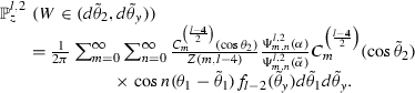
  • (i) For Case I, we only verify for $l\ge 4$ and $v=1$. In this situation the distribution reads as

    $$\begin{aligned} \mathbb {P}^{l,1}_z(W\in d\tilde{\theta }_y)=\sum ^{\infty }_{m=0}\frac{\Psi ^{l,1}_{m,0}(\alpha )}{\Psi ^{l,1}_{m,0}(\tilde{\alpha })}\frac{C^{\left( \frac{l-3}{2}\right) }_m(\cos \tilde{\theta }_2)}{Z(m,l-3)}C_m^{\left( \frac{l-3}{2}\right) }(\cos \theta _2)f_{l-1}(\tilde{\theta }_y)d\tilde{\theta }_y, \end{aligned}$$

    where $\alpha \le \tilde{\alpha }$, $\tilde{\theta }_2 \in [0,\pi )$ and

    $$\begin{aligned} f_{\nu }(\psi )=\frac{1}{\Omega _{\nu }}\sin ^{\nu -2}\psi _1\sin ^{\nu -3}\psi _2\cdots \sin \psi _{\nu -2}. \end{aligned}$$

    (4.63)

    Thus, we have that this distribution integrates to one with a same discussion as in [3] Remark 2.11.

  • (ii) For Case II, we mean $l=4$ and $v=2$. According to Remark 4.1, the distribution for this situation is

    $$\begin{aligned} \begin{array}{ll} \mathbb {P}^{4,2}_{z} &{} (W\in (d\tilde{\theta }_1,d\tilde{\theta }_2))\\ &{} =\frac{1}{4\pi ^2}+\sum ^{\infty }_{m,n=1}\cos m(\theta _1-\tilde{\theta }_1)\cos n(\theta _2-\tilde{\theta }_2)\frac{\Psi ^{4,2}_{m,n}(\alpha )}{\Psi ^{4,2}_{m,n}(\tilde{\alpha })}d\tilde{\theta }_1d\tilde{\theta }_2. \end{array} \end{aligned}$$

    Hence,

    $$\begin{aligned} \begin{array}{ll} \int ^{2\pi }_0\int ^{2\pi }_0\mathbb {P}^{4,2}_{z}(W\in (d\tilde{\theta }_1,d\tilde{\theta }_2)) &{} =\int ^{2\pi }_0\int ^{2\pi }_0\frac{1}{4\pi ^2}d\tilde{\theta }_1d\tilde{\theta }_2\\ &{} =1. \end{array} \end{aligned}$$

  • (iii) For Case III, we only verify for $l>4$ and $l=2$ as in Case I. According to Remark 4.1, the expression of the distribution is

    

    By rotational invariance, we can assume that $\theta _2=0$. Observing that $C^{\left( \frac{l-4}{2}\right) }_m(1)=\left( {\begin{array}{c}l+m-5\\ m\end{array}}\right)$, by the orthogonality of trigonometric functions and Gegenbauer polynomials we have

    $$\begin{aligned} \begin{array}{ll} \int ^{2\pi }_0\int ^{\pi }_0 \cdots &{} \int ^{\pi }_0\int ^{2\pi }_0\mathbb {P}^{l,2}_z\left( W\in (d\tilde{\theta }_1,d\tilde{\theta }_y)\right) \\ &{}= \frac{1}{2\pi }\int ^{2\pi }_0\left( \sum ^{\infty }_{n=0}\cos n(\theta _1-\tilde{\theta }_1)\sum _{m=0}^{\infty }\frac{\Psi ^{l,2}_{m,n}(\alpha )}{\Psi ^{l,2}_{m,n}(\tilde{\alpha })}\left( {l+m-5}{m}\right) \right. \\ &{} \quad \left. \times \,\int ^{\pi }_0\cdots \int ^{\pi }_0\int ^{2\pi }_0\frac{C^{\left( \frac{l-4}{2}\right) }_m(\cos \tilde{\theta }_2)}{Z(m,l-4)}f_{l-2}(\tilde{\theta }_y)d\tilde{\theta }_y\right) d\tilde{\theta }_1\\ &{}= \frac{1}{2\pi }\sum ^{\infty }_{n=0}\int ^{2\pi }_0\left( \cos n(\theta _1-\tilde{\theta }_1)\sum ^{\infty }_{m=0}\frac{\Psi ^{l,2}_{m,n}(\alpha )}{\Psi ^{l,2}_{m,n}(\tilde{\alpha })}\cdot \frac{\Omega _{l-3}}{\Omega _{l-2}}\cdot \frac{2m+l-4}{l-4}\right. \\ &{} \quad \left. \times \,\int ^{\pi }_0C^{\left( \frac{l-4}{2}\right) }_m(\cos \tilde{\theta }_2)\sin ^{l-4}\tilde{\theta }_2d\tilde{\theta }_2\right) d\tilde{\theta }_1\\ &{}= \frac{1}{2\pi }\sum ^{\infty }_{n=0}\int ^{2\pi }_0\left( \cos n(\theta _1-\tilde{\theta }_1)\frac{\Psi ^{l,2}_{0,n}(\alpha )}{\Psi ^{l,2}_{0,n}(\tilde{\alpha })}\cdot \frac{\Omega _{l-3}}{\Omega _{l-2}}\right. \\ &{} \quad \left. \times \,\int ^{\pi }_0C^{\left( \frac{l-4}{2}\right) }_0(\cos \tilde{\theta }_2)\sin ^{l-4}\tilde{\theta }_2d\tilde{\theta }_2\right) d\tilde{\theta }_1\\ &{}= \frac{1}{2\pi }\sum ^{\infty }_{n=0}\int ^{2\pi }_0\frac{\Psi ^{l,2}_{0,n}(\alpha )}{\Psi ^{l,2}_{0,n}(\tilde{\alpha })}\cos n(\theta _1-\tilde{\theta }_1)d\tilde{\theta }_1\\ &{}= \frac{1}{2\pi }\int ^{2\pi }_0\frac{\Psi ^{l,2}_{0,0}(\alpha )}{\Psi ^{l,2}_{0,0}(\tilde{\alpha })}d\tilde{\theta }_1\\ &{}= 1. \end{array} \end{aligned}$$

  • (iv) For Case IV, we mean $l\ge 6$ and $3\le v\le l-3$. The distribution for this case is

    $$\begin{aligned} \begin{array}{ll} \mathbb {P}^{l,v}_z(d\tilde{\theta }_x,d\tilde{\theta }_y)= &{} \sum ^{\infty }_{n=0}\sum ^{\infty }_{m=0}\left( \frac{C_n^{\left( \frac{v-2}{2}\right) }(\cos \theta _1)}{Z(n,v-2)}\cdot \frac{C_m^{\left( \frac{l-v-2}{2}\right) }(\cos \theta _2)}{Z(m,l-v-2)}\cdot \frac{\Psi ^{l,v}_{m,n}(\alpha )}{\Psi ^{l,v}_{m,n}(\tilde{\alpha })}\right. \\ &{} \left. \times \, C_n^{\left( \frac{v-2}{2}\right) }(\cos \tilde{\theta }_1)C_m^{\left( \frac{l-v-2}{2}\right) }(\cos \tilde{\theta }_2)f_{v-2}(\tilde{\theta }_x)f_{l-v-2}(\tilde{\theta }_y)\right) d\tilde{\theta }_xd\tilde{\theta }_y. \end{array} \end{aligned}$$

    With a similar discussion of integration of the part for Gegenbauer polynomials in Case III, we have

    $$\begin{aligned} \int ^{\pi }_0\cdots \int ^{\pi }_0\int ^{2\pi }_0\int ^{\pi }_0\cdots \int ^{\pi }_0\int ^{2\pi }_0\mathbb {P}^{l,v}_z(d\tilde{\theta }_x,d\tilde{\theta }_y)=1. \end{aligned}$$

Appendix: Calculations of the Laplacian–Beltrami Operator

This appendix is devoted to the calculations of the Laplacian–Beltrami operator restricted on pseudo spheres. First, we consider Laplacian–Beltrami operator restricted on a spacelike pseudo sphere of $\mathbb {R}^3_1$, namely, on the spacelike pseudo sphere

$$\begin{aligned} \mathbb {S}_r^{3,1}=\{X=(x_0,x_1,x_2)\in \mathbb {R}^3_1|-x_0^2+x_1^2+x_2^2=r^2\} \end{aligned}$$

under the relationship given by

$$\begin{aligned} x_0=\eta \sinh \alpha ,\ x_1=\eta \cos \beta \cosh \alpha ,\ x_2=\eta \sin \beta \cosh \alpha , \end{aligned}$$

(4.64)

or

$$\begin{aligned} \eta = \Vert X\Vert ,\ \tanh \alpha =\frac{x_0}{\sqrt{x_1^2+x_2^2}},\ \tan \beta =\frac{x_2}{x_1}. \end{aligned}$$

(4.65)

Thanks to multivariable calculus, we have the expression of $\Delta$ restricted on $\mathbb {S}^{3,1}$. That is,

$$\begin{aligned} \begin{array}{ll} \Delta _{\mathbb {S}}^{3,1}= &{} \left( \frac{\partial ^2\eta }{\partial x_1^2} + \frac{\partial ^2\eta }{\partial x_2^2} - \frac{\partial ^2\eta }{\partial x_0^2} \right) \frac{\partial }{\partial \eta } + \left( \frac{\partial ^2\alpha }{\partial x_1^2} + \frac{\partial ^2\alpha }{\partial x_2^2} -\frac{\partial ^2\alpha }{\partial x_0^2} \right) \frac{\partial }{\partial {\alpha }}\\ &{} + \left( \frac{\partial ^2\beta }{\partial x_1^2} + \frac{\partial ^2\beta }{\partial x_2^2} -\frac{\partial ^2\beta }{\partial x_0^2} \right) \frac{\partial }{\partial \beta } + \left( \left( \frac{\partial \eta }{\partial x_1}\right) ^2+ \left( \frac{\partial \eta }{\partial x_2}\right) ^2 -\left( \frac{\partial \eta }{\partial x_0}\right) ^2 \right) \frac{\partial ^2}{\partial \eta ^2}\\ &{} + \left( \left( \frac{\partial {\alpha }}{\partial x_1}\right) ^2+ \left( \frac{\partial {\alpha }}{\partial x_2}\right) ^2 -\left( \frac{\partial {\alpha }}{\partial x_0}\right) ^2 \right) \frac{\partial ^2}{\partial {\alpha }^2} \\ &{} + \left( \left( \frac{\partial \beta }{\partial x_1}\right) ^2+ \left( \frac{\partial \beta }{\partial x_2}\right) ^2 -\left( \frac{\partial \beta }{\partial x_0}\right) ^2 \right) \frac{\partial ^2}{\partial \beta ^2}\\ &{} +\, 2 \left( \frac{\partial \eta \partial {\alpha }}{\partial x_1^2} + \frac{\partial \eta \partial \alpha }{\partial x_2^2} -\frac{\partial \eta \partial \alpha }{\partial x_0^2} \right) \frac{\partial ^2}{\partial \eta \partial \alpha } + 2 \left( \frac{\partial \alpha \partial \beta }{\partial x_1^2} + \frac{\partial \alpha \partial \beta }{\partial x_2^2} -\frac{\partial \alpha \partial \beta }{\partial x_0^2} \right) \frac{\partial ^2}{\partial \alpha \partial \beta }\\ &{} +\, 2 \left( \frac{\partial \beta \partial \eta }{\partial x_1^2} + \frac{\partial \beta \partial \eta }{\partial x_2^2} -\frac{\partial \beta \partial \eta }{\partial x_0^2} \right) \frac{\partial ^2}{\partial \beta \partial \eta }. \end{array} \end{aligned}$$

(4.66)

To calculate the Laplacian $\Delta$ in spacelike coordinates, we only need to calculate the partial differentials on the right hand side of equality (4.66). By (4.65), we get

$$\begin{aligned} \begin{array}{lll} \frac{\partial \eta }{\partial x_0}=-\frac{x_0}{\eta }, &{}\frac{\partial \eta }{\partial x_1}=\frac{x_1}{\eta }, &{}\frac{\partial \eta }{\partial x_2}=\frac{x_2}{\eta }, \\ \frac{\partial \alpha }{\partial x_0}=\frac{\sqrt{\eta ^2+x_0^2}}{\eta ^2}, &{}\frac{\partial \alpha }{\partial x_1}=-\frac{x_0x_1\cosh ^2\alpha }{(\eta ^2+x_0^2)^{3/2}}, &{}\frac{\partial \alpha }{\partial x_2}=-\frac{x_0x_2\cosh ^2\alpha }{(\eta ^2+x_0^2)^{3/2}}, \\ \frac{\partial \beta }{\partial x_0}=0, &{}\frac{\partial \beta }{\partial x_1}=-\frac{x_2}{\eta ^2+x_0^2}, &{}\frac{\partial \beta }{\partial x_2}=\frac{x_1}{\eta ^2+x_0^2}, \\ \frac{\partial ^2\eta }{\partial x_0^2}=-\frac{\eta ^2+x_0^2}{\eta ^3}, &{}\frac{\partial ^2\eta }{\partial x_1^2}=\frac{\eta ^2-x_1^2}{\eta ^3}, &{}\frac{\partial ^2\eta }{\partial x_2^2}=\frac{\eta ^2-x_2^2}{\eta ^3}, \\ \frac{\partial ^2\alpha }{\partial x_0^2}=\frac{2x_0\sqrt{\eta ^2+x_0^2}}{\eta ^4}, &{}\frac{\partial ^2\alpha }{\partial x_1^2}=\frac{2x_0x_1^2(\eta ^2+x_0^2)-x_0x_2^2\eta ^2}{\eta ^4(\eta ^2+x_0^2)^{3/2}}, &{}\frac{\partial ^2\alpha }{\partial x_2^2}=\frac{2x_0x_2^2(\eta ^2+x_0^2)-x_0x_1^2\eta ^2}{\eta ^4(\eta ^2+x_0^2)^{3/2}}, \\ \frac{\partial ^2\beta }{\partial x_0^2}=0, &{}\frac{\partial ^2\beta }{\partial x_1^2}=\frac{2x_1x_2}{(\eta ^2+x_0^2)^2}, &{}\frac{\partial ^2\beta }{\partial x_2^2}=-\frac{2x_1x_2}{(\eta ^2+x_0^2)^2}. \end{array} \end{aligned}$$

Thus, the coefficients in the partial differential operators in (4.66) are

$$\begin{aligned} \frac{\partial ^2\eta }{\partial x_1^2}+\frac{\partial ^2\eta }{\partial x_2^2}-\frac{\partial ^2\eta }{\partial x_0^2}&=\frac{2}{\eta }, \\ \frac{\partial ^2\alpha }{\partial x_1^2}+\frac{\partial ^2\alpha }{\partial x_2^2}-\frac{\partial ^2\alpha }{\partial x_0^2}&=-\frac{\tanh \alpha }{\eta ^2}, \\ \frac{\partial ^2\beta }{\partial x_1^2}+\frac{\partial ^2\beta }{\partial x_2^2}-\frac{\partial ^2\beta }{\partial x_0^2}&=0,\\ \left( \frac{\partial \eta }{\partial x_1}\right) ^2+ \left( \frac{\partial \eta }{\partial x_2}\right) ^2 -\left( \frac{\partial \eta }{\partial x_0}\right) ^2&=1,\\ \left( \frac{\partial \alpha }{\partial x_1}\right) ^2+ \left( \frac{\partial \alpha }{\partial x_2}\right) ^2 -\left( \frac{\partial \alpha }{\partial x_0}\right) ^2&=\frac{1}{\eta ^2\cosh ^2\alpha },\\ \left( \frac{\partial \beta }{\partial x_1}\right) ^2+ \left( \frac{\partial \beta }{\partial x_2}\right) ^2 -\left( \frac{\partial \beta }{\partial x_0}\right) ^2&=-\frac{1}{\eta ^2}, \end{aligned}$$

while the coefficients of the cross terms are zeros.

Then the Laplacian–Beltrami operator $\Delta$ restricted on $\mathbb {S}^{3,1}$ can be expressed in coordinates $(\eta ,\alpha ,\beta )_{\mathbb {S}}$ as

$$\begin{aligned} \Delta _{\mathbb {S}}^{3,1}=\left( \frac{2}{\eta }\frac{\partial }{\partial \eta }+\frac{\partial ^2}{\partial \eta ^2}\right) -\left( \frac{\tanh \alpha }{\eta ^2}\frac{\partial }{\partial \alpha }+\frac{1}{\eta ^2}\frac{\partial ^2}{\partial \alpha ^2}\right) +\frac{1}{\eta ^2\cosh ^2\alpha }\frac{\partial ^2}{\partial \beta ^2}, \end{aligned}$$

while the Laplacian–Beltrami operator restricted on $\mathbb {S}^{3,1}_r$ is expressed as

$$\begin{aligned} \Delta _{sr}^{3,1}=-\frac{1}{r^2}\left( \tanh \alpha \frac{\partial }{\partial \alpha }+\frac{\partial ^2}{\partial \alpha ^2}\right) +\frac{1}{r^2}\frac{1}{\cosh ^2\alpha }\frac{\partial ^2}{\partial \beta ^2}. \end{aligned}$$

(4.67)

Now return to the general case $\mathbb {R}^l_v$. Letting $x=(x_1,x_2,\ldots ,x_v)$ and $y=(y_1,y_2,\ldots ,y_{l-v})$, for any point $X\in \mathbb {S}^{l,v}$ we have

$$\begin{aligned} -\sum _{i=1}^vx_i^2+\sum _{j=1}^{l-v}y_j^2=\eta ^2>0. \end{aligned}$$

Again, we use the coordinates similar to $(\cdot ,\cdot ,\cdot )_{\mathbb {S}}$, namely, a system of coordinates $(\eta ,\alpha ,\theta _y,\theta _x)_{\mathbb {S}}$ satisfying

$$\begin{aligned} \begin{array}{ll} &{} \eta ^2=-\sum _{i=1}^vx_i^2+\sum _{j=1}^{l-v}y_j^2,\\ &{} \tanh ^2\alpha =\frac{\sum _{i=1}^vx_i^2}{\sum _{j=1}^{l-v}x_j^2}, \end{array} \end{aligned}$$

(4.68)

and $\theta _x=(\theta _{x,1},\ldots ,\theta _{x,v-1})$, $\theta _y=(\theta _{y,1},\ldots ,\theta _{y,l-v-1})$ are the standard polar coordinates on the Euclidean unit sphere $\mathcal {S}^{v-1}$ and $\mathcal {S}^{l-v-1}$ respectively. Thus the Laplacian–Beltrami operator restricted on $\mathbb {S}^{l,v}$ with $l\ge 4$ can be expressed as

$$\begin{aligned} \begin{array}{ll} \Delta _{\mathbb {S}}^{l,v}= &{} \left( \frac{\partial ^2}{\partial \eta ^2}+\frac{l-1}{\eta }\frac{\partial }{\partial \eta }\right) \\ &{} -\,\frac{1}{\eta ^2}\left( \frac{\partial ^2}{\partial \alpha ^2}+[(l-v-1)\tanh \alpha +(v-1)\coth \alpha ]\frac{\partial }{\partial \alpha }\right) \\ &{} +\,\frac{1}{\eta ^2\cosh ^2\alpha }\Delta _{\mathcal {S}^{l-v-1}}-\frac{1}{\eta ^2\sinh ^2\alpha }\Delta _{\mathcal {S}^{v-1}}, \end{array} \end{aligned}$$

(4.69)

where $\Delta _{\mathcal {S}^n}$ is the Laplacian operator on the n-dimensional unit sphere.

References

Cohen de Lara, M.: On drift, diffusion and geometry. J. Geom. Phys. 56(8), 1215–1234 (2006)
Cammarota, V., De Gregorio, A., Macci, C.: On the asymptotic behavior of the hyperbolic Brownian. J. Stat. Phys. 154(6), 1550–1568 (2013)
Cammarota, V., Orsingher, E.: Hitting spheres on hyperbolic spaces. Theory Probab. Appl. 57(3), 419–443 (2013)
Dunkel, J., Hänggi, P.: Relativistic Brownian motion. Phys. Rep. 471(1), 1–73 (2009)
Dembo, A., Peres, Y., Rosen, J.: Brownian motion on compact manifolds: cover time and late points. Electron. J. Probab. 8(15), 1–14 (2003)
Dembo, A., Peres, Y., Rosen, J., Zeitouni, O.: Cover times for Brownian motion and random walks in two dimensions. Ann. Math. 160(2), 433–464 (2004)
Grigor’yan, A.: Analytic and geometric background of recurrence and non-explosion of the Brownian motion on Riemannian manifolds. Bull. Am. Math. Soc. 36, 135–249 (1999)
Garbaczewski, P.: Rotational diffusions as seen by relativistic observers. J. Math. Phys. 33(10), 3393–3401 (1992)
Gradshteyn, I.S., Ryzhik, I.M.: Table of Integrals, Series, and Products, 4th edn. Academic Press, New York (1981)
Itô, K.: On stochastic differential equations on a differential manifold I. Nagoya Math. J. 1, 35–47 (1950)
Lablée, O.: Spectrual Theory in Riemannian Geometry. European Mathematical Society (EMS), Zurich (2015)
Morava, J.: Conformal invariants of Minkowski space. Proc. Am. Math. Soc. 95, 565–570 (1985)
Mckean, H.P.: Stochastic Integrals. Academic Press, New York (1969)
Mizrahi, S., Daboul, J.: Squeezed states, generalized Hermitz polynomials and pseudo-diffusion equation. Phys. A 189, 635–650 (1992)
Øksendal, B.: Stochastic Differential Equations, an Introduction with Applications, 6th edn. Springer, New York (2003)
O’Hara, P., Rondoni, L.: Brownian motion in Minkowski space. Entropy 17, 3581–3594 (2015)
O’neill, B.: Semi-Riemannian Geometry with Applications to Relativity. Academic Press, New York (1983)
Polyanin, A.D., Zaitsev, V.F.: Handbook of Exact Solution for Ordinary Differential Equations. Chapman & Hall, Boca Raton (2003)
Szegö, G.: Orthogonal Polynomials, 4th edn. AMS, Providence (1975)
Acknowledgments
We thank the anonymous referees for their valuable suggestions and comments.
Author information
Authors and Affiliations
Corresponding author
Additional information
This work was supported by National Basic Research Program of China (Grant No. 2013CB834100), National Natural Science Foundation of China (Grant No. 11571065), and National Natural Science Foundation of China (Grant No. 11171132). Xiaomeng Jiang is supported by a foundation. The foundation number is National Natural Science Foundations of China (Grant No. 11301541).