
Abstract
In recent years, intellectualized technology has gradually matured, and it has been applied to all aspects of life. Among them, the emerging industry represented by smart home is rising, but the current smart home industry cannot meet people’s demand because of the immature technology, high cost for maintenance and price. In the situation, this paper presents a decision method for user’s behaviours which based on the C4.5 algorithm, selecting samples from data collected by intelligent home system, analysing and processing samples to generate a decision tree. According to the user’s living habits, the decision tree is used to help users make decisions, so as to provide users with more intelligent and efficient services.
1 Introduction
Smart home is a product of the IoT (Internet of Things) that use comprehensive wiring technology, network communications and automatic control technology to build an efficient management system for daily affairs in the family. It aims at improving home safety comfort and convenience [1].
The concept of smart home has been proposed since the 1980s, however, today we has not achieved much success. The current domestic smart home appliances mostly are displayed as exhibits in the science and technology museum, which does not complete the transition as a commodity. Despite the high cost, at this stage, the system can only control household facilities simply, to the extent we can see, it cannot meet user’s demand well. What a perfect smart home needs to do is to take the initiative to provide service for the user, and effectively solve the actual needs and ease of use.
The intelligent home control and sensing system is based on the IoT platform, which consist of various sensor nodes and relays. In the System, the sensor nodes can sense and gather information from environment. And according to the sensor data, the relays have a function to control household appliances. All the sensor data and household appliances control records will be transmitted to the server database.
In this paper, we propose an implementation of the C4.5 algorithm to classifying data in the intelligent home control and sensing system. It based on the related data set classification and computing operations is used to generate the decision tree which can describe the user’s behavioral habit. According to the data and current environment parameters, the system can help users make decisions. All of the data from sensors are collected in server database thus the classification progress occurs in server, we extract a random collection of samples from the database to build a decision model, and found out the relationship between environmental parameters and the user’s habits.
This paper is divided into six chapters. The first chapter describes the background and current status of smart home industry, the composition and working principle of intelligent home control and sensing system in this article are introduced in this article. And so as the improvements in the system with the decision tree algorithm.
The second chapter describes the data mining technology, including the purpose of data mining technology, processes, and some of the main analysis methods. The basic principle of decision tree algorithm and decision tree algorithm in data mining are given detailed description.
The third chapter introduces ID3 and C4.5 algorithm, as well as the basic principles of the two algorithms. Comparing the ID3 algorithm and the C4.5 algorithm shows the difference between the two algorithms and the improvement of C4.5 algorithm.
The fourth chapter is a description of the decision tree construction process. The process principle of C4.5 algorithm is described step by step, then introduce the data processing of C4.5 algorithm in the system through instances by taking 15 operation records as an example. The processing are describes into two parts: the pre-processing of the sample set and the decision tree generation.
The fifth chapter is the experiment chapter, in which the decision rules are extracted from the decision tree generated by the algorithm, and the accuracy and time costing of the generated decision tree are tested by two groups of different numbers.
The sixth chapter is a summary of the whole paper, it includes the effection of C4.5 algorithm in intelligent home control and sensing system, and the shortcomings it shows in the experiment.
2 Theoretical Basis
2.1 Data Mining
The concept of data mining was presented at the first international conference on intellectual discovery and data mining in Canada in 1995. As a product of multidisciplinary comprehensive, the purpose of data mining is to extract the unknown, potentially useful information and knowledge from a large number of incomplete and noisy application data [2].
Data mining technology can analyse data warehouse data in a highly automated way, making inductive reasoning, dig out potential patterns, and utilize the existing information and data for maximum efficiency. Through data mining, the valuable knowledge and rules, or a high level of information will be extracted from the database related collection, and displayed in different aspects, to help decision makers to make reasonable and correct decisions [3]. The data analysis methods commonly used in data mining include classification, regression analysis, clustering, association rules, characteristics, deviation analysis, etc.
Data mining consists of three stages: data preparation stage, data mining stage, result evaluation and expression stage. Data preparation stage is mainly to complete the selection of a large amount of data, purification, conversion, works in this stage will affect the effectiveness of the final model and the efficiency and accuracy of data mining, useless information can be eliminated in the process of mining [4]. Data mining stage firstly need to select the appropriate mining algorithm, such as decision trees, classification, clustering and rough set, and then analyse the data from the former stage to build the knowledge model. And the main work in result evaluation and expression stage is to find effectiveness of the knowledge model through the result verification, and interpret the results and report writing.
2.2 The Decision Tree
The decision tree is a common kind of data mining classification methods, it can classify data into specific classes by attribute values of objects. The classification algorithm mainly obtains the collection of input data objects and output the classified objects. The goal of the algorithm is to classify each object accurately into the corresponding class, typically, the conditional attribute set of the object is assumed to be known. In general, classification requires two steps: first step, construct the classifier [5]. Create a classification model through the classification algorithm, and the model is based on the analysis of the training sample data. Usually, classification model is performed into mathematical formula, classification rules or decision tree. When the classifier is constructed, then it needs to be evaluated to ensure its accuracy and used to predict the unknown classification data. The second step is to label data by using the classifier, and get the whole classification of the data at the final.
The decision tree algorithm in classification adopts the top–down approach, using instances as a training set to build a training model. Its main purpose is to find the correlation from a group of disordered data with no rule [6, 7]. Decision tree is a non-parametric pattern recognition technique, commonly used for classification and prediction. With high accuracy and fast learning characteristics [8], the decision tree algorithm is one of the most widely used inductive reasoning methods, which can handle the noise part of the training set, and learn the separation expression of the discrete value function.
Decision tree is a structure with two kinds of node, the leaf node and the decision node. The decision node provides relevant execution on each attribute value, with a branch and sub tree for each possible output of the test. It is mostly terminated at the leaf node, and the leaf node points to different results for each different situation of the test, the decision can made by the results got from the decision tree [9].
The basic principle of the decision tree learning is to find out the attribute can classify data mostly, it starts building a decision tree from the root node [10, 11]. The number of node attribute values defines its own branches to other nodes, and each branch can has a new node, the branch nodes finally end in the leaf nodes, then the leaf nodes lead to the labelled cases. Therefore, a decision tree is constructed from the root node with dataset, and moved to the corresponding attribute values of tree branches, and each branch has its own classification standard, which will point to a new node, this process will be repeated in the process of building [12].
3 The C4.5 Algorithm
The ID3 algorithm is a decision tree algorithm of machine learning algorithms, proposed by Ross Quinlan in 1986 [13]. The ID3 algorithm is a recursive process of data structure decision tree, which applies Shannon’s information theory into decision tree algorithm [14]. The information theory is put forward by learning from the concept of entropy in thermodynamics, entropy is a measure of unpredictable data, which is defined as the average amount of information produced by a stochastic source of data. It solved the quantization of information, using the entropy describes the source of uncertainty and the measurement message contained in the amount of information.
The ID3 algorithm uses the information entropy as the criterion for selecting test properties, classifying the training entity sets, and constructing decision trees to classify the entire instance space by the test attribute. In the construction progress, a property is selected to apart the data to have mostly same class values of the data on the child nodes. If the data on a node is evenly distributed, the node will have the maximum entropy and vice versa [15, 16].
The C4.5 algorithm is an optimization of the ID3 algorithm [17], which utilizes the concept of information gain and entropy. Using information acquisition as the main partition standard of the partition node and build the decision tree. The information gain usually is used in information theory to describe the homogeneity of data samples. The essence of C4.5 algorithm is to calculate the information gain ratio of each attribute from the sample set, and generate a decision tree according to each information gain ratio [18]. As a result, the algorithm generates a multi-level classifier in the form of a tree, which divides the data into different classes, each class performs as a node, and each node can have one or more child nodes except the leaf nodes, through to the classification standard, the data sets are divided into different nodes until the leaf nodes, then every leaf node points to a label, thus reaching the effect of the decision [19].
C4.5 algorithm and ID3 algorithm basically have the same process, the main difference between them is the attribute selection criteria [20]. The ID3 algorithm takes the information gain as the criterion, and the C4.5 algorithm takes information gain ratio. For selecting the maximum information gain ratio as the classification attribute, it can overcome the disadvantage of the information gain tendency of multi-value attribute selection [21].
4 Analysis of User Behavior and Decision
4.1 Steps of the C4.5 Algorithm
Assume that set D is the sample training set, and set D has n attributes, D{A1, A2, …, An}. An is the target class, which has j values. Pi (1 ≤ i ≤ j) is the probability of tuples in An, The information entropy calculation formula of the training set is as follows.
And assume that class B is one of attributes in D, class B has n different values dividing training set D into n subsets with B{D1, D2, …, Dn}, calculate each subset’s information entropy Info(Dm) (1 ≤ m ≤ n) with calculation formula (1) in step (1). In the sample training set D, class B ‘s information expectation InfoB (D) calculation formula is as follows.
\(\left| {{\text{D}}_{\text{m}} } \right|\,\,{\text{and}}\,\,\left| {\text{D}} \right|\) in the Eq. (2) are the number of D m and D tuples.
In step (1) and step (2), the information entropy and information expectation is calculated, then the information gain GainB of class B is needed to be calculated, the formula is as follows.
The split information SplitEB of class B calculation formula is as follows [22, 23].
Through the step (3) and step (4) above, we have the information gain GainB and the split information SplitEB, so the information gain ratio of class B calculation formula is as follows.
Repeating step (1) to step (5), calculate every class’s information gain ratio, comparing each class’s information gain ratio, we get the largest class of the information gain ratio, which is considered to be the root node of the decision tree.
The number of the class’s attributes determines the number of the root node’s branches, which means that if the class has n attributes, then the root node has that branches. And each branch should repeats step (1) through step (6) to select the most appropriate node as a branch node, and this progress will be repeated till reach the leaf node, finally, paste the result label for the leaf node.
4.2 Data Pre-process
There is a large amount of redundancy in the data stored in the system database, and the data needs to be pre-processed to improve the accuracy of the conclusion. The database records include the personal account information, temperature, CO2 concentration, PM 2.5, humidity, the home appliance operation records and other environmental parameters. In this scenario, only a part of the database record is used to build the decision tree. At the same time, considering the timeliness of user habits and changes in the four seasons, only the most recent year’s records are selected for training.
And due to the database haves a lot of irrelevant attributes, such as personal information, CO2 concentration and so on, which have nothing to do here needed to remove. Finally, four properties of time, temperature, humidity and operation records are selected. The time attribute has day and night two values, the temperature attribute has cold, warmer, moderate and hot four values, the humidity attribute has dry, semi-moisture and wet three values, the operation records has AC (refrigeration), AC (Heating) and fan three values for the operation object. But there are also many incorrect records and empty values for the operation records of home appliances or other attributes, these records should be deleted too to ensure the accuracy of the decision tree. In this paper, 15 operation records of air conditioners and fans are selected to illustrate the calculation process, the data records is shown in Table 1 below.
4.3 Decision Tree Generation
-
1.
Calculate the information entropy of the sample target
As Table 1 shows, it contains 15 operation records including AC (heating), AC (refrigeration), fan three categories, among them, the AC (heating) has three records, AC (refrigeration) has four records, and fan has eight records, so we can calculate the target class information entropy Info(D) with formula (1), which is as follows.
$${\text{Info(D)}} = - \mathop \sum \limits_{i = 1}^{3} {\text{p}}_{i} log_{2} {\text{p}}_{i} = -\, \frac{3}{15}\log_{2} \frac{3}{15} - \frac{4}{15}\log_{2} \frac{4}{15} - \frac{8}{15}\log_{2} \frac{8}{15} = 1.46$$ -
2.
Calculate all kinds of information expectations about attributes in the target class
Here we select the time class as an example to describe the calculation process. The time class includes the two attributes: day and night, firstly we should calculate the information entropy of the two properties. During the day attribute, there are nine records, two of which operate on AC (heating), three on AC (refrigeration) and four on the fan. The night attribute has six records, including one record of AC (heating), one record of AC (refrigeration), four records of open fan, the day and night information entropy Info(D)day, Info(D)night are calculated with formula (1) as follows.
$$\begin{aligned} {\text{Info(}}D_{\text{day}} )& = - \mathop \sum \limits_{i = 1}^{3} {\text{p}}_{i} log_{2} {\text{p}}_{i} = -\, \frac{2}{9}\log_{2} \frac{2}{9} - \frac{3}{9}\log_{2} \frac{3}{9} - \frac{4}{9}\log_{2} \frac{4}{9} = 1.53 \\ {\text{Info(}}D_{\text{night}} )& = - \mathop \sum \limits_{i = 1}^{3} {\text{p}}_{i} log_{2} {\text{p}}_{i} = -\, \frac{1}{6}\log_{2} \frac{1}{6} - \frac{1}{6}\log_{2} \frac{1}{6} - \frac{4}{6}\log_{2} \frac{4}{6} = 1.25 \\ \end{aligned}$$As it’s described, the records of day attribute are nine, and the records of night attribute are six, with formula (2), the information expectation of time class in target class Infotime (D) is calculated as follows.
$$Info_{\text{time}} ( {\text{D)}} = \mathop \sum \limits_{m = 1}^{2} \frac{{\left| {D_{m} } \right|}}{\left| D \right|}{\text{Info(}}D_{m} ) = \frac{9}{15}Info(D_{\text{day}} ) + \frac{6}{15}Info(D_{\text{night}} ) = 1.42$$Similarly, the temperature class includes 4 attributes: 3 records of cold, 5 records of warmer, 2 records of moderate and 5 records of hot. The cold attribute has only 3 records of AC (heating). The warmer attribute has 4 records of fan and 1 record of AC (refrigeration).The moderate attribute has only 2 records of fan. The hot attribute has 3 records of AC (refrigeration) and 2 records of fan.
The humidity class include 3 attributes: 9 records of dry, 4 records of semi-moisture and 2 records of wet. The dry attribute has 4 records of AC (refrigeration), 4 records of fan and 1 record of AC (heating). The semi-moisture attribute has 3 records of fan and 1 record of AC (heating). The wet attribute has 1 record of fan and 1 record of AC (heating).
We can calculate temperature and humidity classes’ information expectation, which are: Infotemperature(D) = 0.56, Infohumidity(D) = 1.18.
-
3.
Calculate the information gain
Through step (1) and step (2), we get the target class’s information entropy Info(D) and all information expectations, Infotime (D), Infotemperature(D), Infohumidity(D), about the attributes that the training set contains, then using them to calculate the information gain of the attributes. To describe the computation process, here also take the time attribute to calculate the information gain as an example, the time class information gain Gaintime is calculated by using the formula (3) as follows.
$$Gain_{\text{time}} = Info(D) - Info_{\text{time}} ({\text{D}}) = 0.04$$Similarly, the information gain of temperature and humidity is calculated to be Gaintemperature = 0.9, Gainhumidity = 0.28.
-
4.
Calculate the split information
Also take the time class as an example to describe the computation process. In the sample data set, there are 9 days in the time attribute, six in the night attribute, and SplitEtime is calculated with formula (4) to be as follows.
$$SplitE_{\text{time}} = - \mathop \sum \limits_{m = 1}^{2} \frac{{\left| {D_{m} } \right|}}{\left| D \right|}log_{2} \frac{{\left| {D_{m} } \right|}}{\left| D \right|} = -\, \frac{9}{15}\log_{2} \frac{9}{15} - \frac{6}{15}\log_{2} \frac{6}{15} = 0.97$$Similarly, the temperature class has 3 records of cold, 5 records of warmer, 2 records of moderate and 5 records of hot, and the humidity class has 9 records of dry, 4 records of semi-moisture and 2 records of wet. So, the split information of temperature and humidity is calculated to be SplitEtemperature = 1.91, SplitEhumidity = 1.34.
-
5.
Calculate the information gain ratio
Through the step above, we get the information gain, Gaintime, Gaintemperature, Gainhumidity, and the split information, SplitEtime, SplitEtemperature, SplitEhumidity, of all attributes, and the information gain Ratio is needed to be calculated. Here take the time attribute as an example, the information gain Ratio GainRatiotime is calculated with formula (5) to be as follows.
$$GainRatio_{\text{time}} = \frac{{Gain_{\text{time}} }}{{SplitE_{\text{time}} }} = 0.04$$Similarly, the information gain ratio of temperature and humidity is calculated to be: GainRatiotemperature = 0.47,GainRatiohumidity = 0.21.
-
6.
Choose the most appropriate node
According to the calculation above, the information gain ratio of temperature is the largest, so the temperature attribute is chosen to be the root node of the decision tree.
-
7.
Build the whole decision tree
And because the temperature class has 4 attributes, the root node has four branches, and each branch should repeat step (1) to step (5) calculation process to complete the whole decision tree. Here skip the calculation, the result of the decision tree is shown in Fig. 1.
Fig. 1 
Decision tree
According to the Decision tree constructed above in Fig. 1, we can acquire the decision tree rules, and draw a flowchart of it, as shown in Fig. 2. Based on the conditions, we can follow the flowchart from the start to the end, and get the result generated by the C4.5 algorithm in the decision tree.
Fig. 2 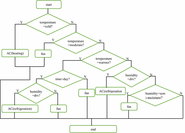
Decision tree flowchart


5 Experiment
The experiment is mainly based on the smart home system database to compare the effect of decision-making, so as to verify the accuracy and performance of C4.5 algorithm. We selected the latest month’s records randomly from the database which is complete and unused, split it into two groups of dataset, one set contains 100 records, and the other set contains 1000 records, and also preprocessed two groups of data. Work though the decision tree to get the classification results of the records, then compare the classification results and target attribute values with the record itself, if same, then the decision is defined right, if two different decision-making occurs, then the decision is wrong. Two sets of data were tested separately, and the accuracy and time costing of the two sets of data were counted. The test results were showed in Table 2.
It can be seen from the chart, two groups of data records have almost equal accuracy in the experiment, This means that the accuracy of the algorithm is not changed by the size of the data, but in terms of time costing, can be found that the more the number of tests, the more time will be taken, and there is a trend of growth in it.
In the system, the information gain ratio is applied to select the attribute as a node in the progress of the C4.5 algorithm, it overcomes the deficiency of the attribute that is more selective when choosing the attribute with information gain [24, 25], and make A more accurate selection of the classification properties of the training set. The sample data set is processed through the C4.5 algorithm to construct a decision tree of user’s behavioural habit, and the decision-making function of the decision tree is showed with realization automatic control of household appliances according to the real-time changes of environmental parameters.
The C4.5 algorithm is only suitable for data sets that can reside in memory, and when the training set is larger than the memory capacity, the algorithm cannot handle it and the program may will have an error in the runtime [26, 27]. Besides that, generating a decision tree is a complex process that requires a lot of computation, the frequency of repetition is very high, during each loop, it generates a decision tree and rebuild the tree in next loop, so the process can consume a lot of resources with low productivity [28].
6 Conclusion
Due to the habits of the differences between individual users, so the data pre-processing stage need to filter the operation subject, make the data with individuality and pertinence to ensure the independence of the individual behaviours.
The advantage of the C4.5 algorithm on this system is that it depends on user’s own behaviours, and it can take the user’s decision automatically before user’s responds. It can “read” the user’s mind, providing convenient and intelligent service.
At the same time, the longer the life cycle, the more accurate the decision-making ability, but also because of this, there is a grinding period between system and user, and during the period, the result may not be very accurate due to the lack of data. The duration of the grinding period is inversely proportional to the user’s use time. The longer the use time, the shorter the duration of the grinding period.
The ID3 algorithm and the C4.5 algorithm in decision tree are classic algorithm has been applied widely. Although the C4.5 algorithm is improved compared with the ID3 algorithm, finding better data processing methods to support decision tree need to be further studied.
References
A. Chakravorty, T. Wlodarczyk, and C. Rong, Privacy preserving data analytics for smart homes. In 2013 IEEE Security and Privacy Workshops, pages 23–27, San Francisco, CA, USA, 2013.
Y. Li, Z. L. Jiang, X. Wang, S. M. Yiu, and P. Zhang, Outsourcing privacy preserving ID3 decision tree algorithm over encrypted data-sets for two-parties. In 2017 IEEE Trustcom/BigDataSE/ICESS, pages 1070–1075 Sydney, NSW, Australia, 2017.
R. Esmailzadeh, Information theory. In Broadband Telecommunications Technologies and Management, pages 376, Wiley Telecom, 1st edition, 2016.
S. Jhajharia, S. Verma, and R. Kumar, A cross-platform evaluation of various decision tree algorithms for prognostic analysis of breast cancer data. In 2016 International Conference on Inventive Computation Technologies (ICICT), pages 1–7, Coimbatore, 2016.
Z. Wen, B. He, D. Xu, and Q. Feng, A method for landslide susceptibility assessment integrating rough set and decision tree: A case study in Beichuan, China. In: 2016 IEEE International Geoscience and Remote Sensing Symposium (IGARSS), pages 4952–4955, Beijing, 2016.
P. Chandrasekar, K. Qian, H. Shahriar, and P. Bhattacharya, Improving the prediction accuracy of decision tree mining with data preprocessing. In 2017 IEEE 41st Annual Computer Software and Applications Conference (COMPSAC), pages 481–484, Turin, 2017.
Z. Yuan, and C. Wang, An improved network traffic classification algorithm based on Hadoop decision tree. In 2016 IEEE International Conference of Online Analysis and Computing Science (ICOACS), pages 53–56, Chongqing, 2016.
N. Hasan, M. T. Uddin, and N. K. Chowdhury, Automated weather event analysis with machine learning. In 2016 International Conference on Innovations in Science, Engineering and Technology (ICISET), pages 1–5, Dhaka, 2016.
B. Sugiarto, and R. Sustika, Data classification for air quality on wireless sensor network monitoring system using decision tree algorithm. In 2016 2nd International Conference on Science and Technology-Computer (ICST), pages 172–176, Yogyakarta, 2016.
M. Vadovský, and J. Paralič, Parkinson’s disease patients classification based on the speech signals. In 2017 IEEE 15th International Symposium on Applied Machine Intelligence and Informatics (SAMI), pages 000321–000326, Herl’any, 2017.
Y. Promdee, S. Kasemvilas, N. Phangsuk, and R. Yodthasarn, Predicting persuasive message for changing student’s attitude using data mining. In 2017 International Conference on Platform Technology and Service (PlatCon), pages 1–5, Busan, 2017.
M. Shafiq, X. Yu, and A. A. Laghari, WeChat text and picture messages service flow traffic classification using machine learning technique. In 2016 IEEE 18th International Conference on High Performance Computing and Communications; IEEE 14th International Conference on Smart City; IEEE 2nd International Conference on Data Science and Systems (HPCC/SmartCity/DSS), pages 58–62, Sydney, NSW, Australia, 2016.
S. Linping, M. Hongtao, M. Yunlang, and C. Rui, The research of classified method of the network traffic in security access platform based on decision tree. In 2016 7th IEEE International Conference on Software Engineering and Service Science (ICSESS), pages 475–480, Beijing, 2016.
Y. Jiarula, et al., Fault mode prediction based on decision tree. In IEEE on Conference Advanced Information Management, Communicates, Electronic and Automation Control, pages 1729–1733, 2017.
Y. Wang, et al., Decision tree based validation of load model parameters. In IEEE Power and Energy Society General Meeting, pages 1–5, 2016.
F. Babič, M. Vadovský, M. Muchová, J. Paralič, L. Majnaric. Simple understandable analysis of medical data to support the diagnostic process. In IEEE, International Symposium on Applied Machine Intelligence and Informatics, 2017.
M. Antonelli, D. Bernardo, H. Hagras and F. Marcelloni, Multiobjective evolutionary optimization of Type-2 fuzzy rule-based systems for financial data classification, IEEE Transactions on Fuzzy Systems, Vol. 25, No. 2, pp. 249–264, 2017.
P. Gong, H. T. Ma, and Y. Wang, Emotion recognition based on the multiple physiological signals. In IEEE International Conference on Real-Time Computing and Robotics, pages 140–143, 2016.
J. Rabcan, M. Vaclavkova, and R. Blasko, Selection of appropriate candidates for a type position using C4.5 decision tree. In 2017 International Conference on Information and Digital Technologies (IDT), pages 332–338, Zilina, 2017.
B. Zhou, C. Cao, C. Li and Y. Cao, Hybrid islanding detection method based on decision tree and positive feedback for distributed generations, Iet Generation Transmission and Distribution, Vol. 9, No. 14, pp. 1819–1825, 2015.
S. P. Abercrombie and M. A. Friedl, Improving the consistency of multitemporal land cover maps using a hidden markov model, IEEE Transactions on Geoscience and Remote Sensing, Vol. 54, No. 2, pp. 703–713, 2016.
M. Vatani, T. Amraee, A. M. Ranjbar and B. Mozafari, Relay logic for islanding detection in active distribution systems, Iet Generation Transmission and Distribution, Vol. 9, No. 12, pp. 1254–1263, 2015.
Z. Zhou, G. Si, J. Chen, K. Zheng, and W. Yue, Application of a novel parallel variable weight decision tree algorithm in transformer fault diagnosis. In 2017 IEEE 2nd Advanced Information Technology, Electronic and Automation Control Conference (IAEAC), pages 467–471, Chongqing, China, 2017.
R. Wang, S. Kwong, X. Z. Wang and Q. Jiang, Segment based decision tree induction with continuous valued attributes, IEEE Transactions on Cybernetics, Vol. 45, No. 7, p. 1262, 2015.
A. R. Al Taleb, M. Hoque, A. Hasanat, and M. B. Khan, Application of data mining techniques to predict length of stay of stroke patients. In 2017 International Conference on Informatics, Health and Technology (ICIHT), pages 1–5, Riyadh, 2017.
E. K. Hashi, M. S. U. Zaman, and M. R. Hasan, An expert clinical decision support system to predict disease using classification techniques. In 2017 International Conference on Electrical, Computer and Communication Engineering (ECCE), pages 396–400, Cox’s Bazar, 2017.
S. Wongcharoen, and T. Senivongse, Twitter analysis of road traffic congestion severity estimation. In 2016 13th International Joint Conference on Computer Science and Software Engineering (JCSSE), pages 1–6, Khon Kaen, 2016.
G. P. Seneviratne, and M. G. U. Nadeeshani, An empirical approach towards the knowledge extraction in a high-dimensional clinical data set. In 2017 IEEE 7th International Advance Computing Conference (IACC), pages 132–137, Hyderabad, 2017.
Author information
Authors and Affiliations
Corresponding author
Rights and permissions
About this article

Cite this article
Xie, L., Xu, F. The Research of User’s Behavioural Decision on Intelligent Home Control and Sensing System. Int J Wireless Inf Networks 25, 250–257 (2018). https://doi.org/10.1007/s10776-018-0383-6
Received:
Accepted:
Published:
Issue Date:
DOI: https://doi.org/10.1007/s10776-018-0383-6