Quantum Theory is an Information Theory

Abstract

In this paper we review the general framework of operational probabilistic theories (OPT), along with the six axioms from which quantum theory can be derived. We argue that the OPT framework along with a relaxed version of five of the axioms, define a general information theory. We close the paper with considerations about the role of the observer in an OPT, and the interpretation of the von Neumann postulate and the Schrödinger-cat paradox.

1 Introduction

After the experience accumulated in the field of Quantum Information theory, in the last decade a completely new perspective on foundations of Quantum Theory flourished. The possibilities introduced in information processing by shifting from the classical to the quantum computation paradigm opened an unexpected scenario containing novel algorithms [3, 9], protocols [2], and properties of information [10, 11]. The new approach to quantum foundations started from this standpoint, and aimed at upturning the role of the astonishing theorems of quantum information to basic principles from which the Hilbert space structure of the theory could be derived [6–8]. Moreover, a crucial feature of the new foundational approach was the idea that the transition from classical to quantum information highlights only a tiny fraction of the general features of information [1], whereas a thorough approach would also clearly locate the boundaries of a general information theory.

Quantum Theory is indeed derived as a special theory of information, from six information-theoretical principles [5] that, for the first time, also set the boundaries of a general theory of information. The power of the new principles resides not only in the reformulation of quantum theory, but also in providing a framework and a language for deriving the most relevant theorems of quantum theory and of quantum information theory, using a conceptual path instead of a mathematical derivation.

In the present paper we review the formulation of the information-theoretical principles. We first set the framework and the language of the operational probabilistic theory (OPT), which also defines the background scenario of a general information theory [4]. We then use the language to express the six principles, five of which are fulfilled also by classical information. The purification principle is the one that singles out quantum theory.

The OPT framework, in addition to allowing a thorough definition of a general information processing, along with some of the principles also represent an essential part of the scientific method itself, being such principles strictly needed in order to do physics. With minimal relaxation and generalization, this is true for all the five principles shared by classical information. The OPT framework and the new principles will become the standpoint for further progresses in the exploration or modification of the most fundamental theory in physics.

2 The General Framework

One of the main rules of the scientific method is to have well clear distinction between what is experimental and what is theoretical. Though this would seem a trivial statement, such a confusion happens to be often the source of disagreement between scientists. Though the description of the apparatus is generally intermingled with theoretical notions, the pure experimental datum must have a conventionally defined “objectivity” status, corresponding to “openly known” information, shareable by any number of different observers. Then both the theoretical language and the framework must reflect this theory–experiment distinction, by indicating explicitly which notions are assigned such objectivity status. Logic, with the Boolean calculus of events, is an essential part of the language, and Probability Theory can be regarded as an extension of logic, assigning probabilities to events. The notion that is promoted to the objectivity status is that of “outcome”, announcing which event of a complete test occurred. The operational framework is a further extension of probability theory that provides a theoretical connectivity between events, the outcome remaining the only ingredient that is granted the objectivity status: everything else—probabilities, events, and their connectivity—remain purely theoretical.

A test is a collection $\{ \mathscr {C}_i \}_{i \in \mathrm {X}}$ of possible events $\mathscr {C}_i$ labeled by outcomes $i\in \mathrm {X}$, and has an input system $\mathrm {A}$ and an output system $\mathrm {B}$. We can denote it through a diagram as follows

Each outcome $i \in \mathrm {X}$ corresponds to a possible event, represented as

The run of two tests $\{\mathscr {C}_i\}$ and $\{\mathscr {D}_j\}$ in a sequence is a new test called sequential composition of $\{\mathscr {C}_i\}$ and $\{\mathscr {D}_j\}$, whose events are

while their run in parallel is named parallel composition of $\{\mathscr {C}_i\}$ and $\{\mathscr {D}_j\}$, with events

with composite input system $\mathrm {A}\mathrm {C}$ and output $\mathrm {B}\mathrm {D}$. Since parallel composition represents the independent run of two tests on different systems, the sequential composition of two tests that are parallel compositions must satisfy the following intuitive property

Parallel composition of tests clearly requires a notion of composition of systems. Given any two systems $\mathrm {A}$ and $\mathrm {B}$, one can form the composite system $\mathrm {A}\mathrm {B}$. Composition is associative: $(\mathrm {A}\mathrm {B})\mathrm {C}=\mathrm {A}(\mathrm {B}\mathrm {C})$. In every experiment one can involve a trivial system, denoted as $\mathrm {I}$, that is a virtual system that carries no information. Since this system is trivial, we have $\mathrm {A}\mathrm {I}=\mathrm {I}\mathrm {A}=\mathrm {A}$.

The tests that have the trivial system as input or output system, are called preparation tests and observation tests, respectively, and will be denoted as follows

Merging the outcomes of one test into composite outcomes of a coarse-grained test, or refining compatible tests are primitives that need to be accounted for. Probability theory enters the framework in assigning a joint probability to events. Keeping track of the connectivity between events corresponds to set a correspondence between the joint probability and the closed network of events, namely an event with trivial input and output systems. Hence, the probability is an event of the trivial system $\mathrm {I}$, and this corresponds to associate a closed diagram to a number $0\le P\le 1$ as follows

This also corresponds to have the joint probability of all outcomes parametrically dependent from the circuit, namely

$$\begin{aligned} P=p\big (i_1,i_2,i_3,i_4,i_5,i_6,i_7,i_8|\Psi ,\mathscr {A},\mathscr {B},\mathscr {C},\mathscr {D},\mathscr {E},\mathscr {F},G\big ). \end{aligned}$$

We emphasize that, whereas the outcomes are objective, the association of a mathematical object to the joint event, the identification of systems, and the assessment of the probability of the event are purely theoretical ingredients. Thus the general element of the OPT theory is the joint probability and its parametric dependence on the circuit.

2.1 States, Effects, Transformations

Consider now the following diagram

The fact that the diagram corresponds to a real number implies that one can think of the observation-event $a_j$ as a functional on preparation-events $\rho _i$, and viceversa a preparation-event $\rho _i$ is a functional on observation events $a_j$. If two preparation-events $\rho _i$ and $\sigma _{i'}$ have the same probabilities for all observation-events $a_j$, we will say that they prepare the same state, and similarly if two observation-events have the same probabilities for all preparation-events $\rho _i$, we will say that they detect the same effect. Since preparing the same state and detecting the same effect are equivalence relations, we will collect preparation-events and observation-events into equivalence classes called states and effects, respectively, and identify them with the corresponding functionals. States and effects are then elements of real vector spaces $\mathsf {St}_\mathbb {R}(\mathrm {A})$ and $\mathsf {Eff}_\mathbb {R}(\mathrm {A})$, that will be assumed to be finite dimensional, with dimension $D_\mathrm {A}$. The dimension $D_\mathrm {A}$ is the size of system $\mathrm {A}$, and thus we will say that $\mathrm {B}$ is smaller than $\mathrm {A}$ if $D_\mathrm {B}<D_\mathrm {A}$. The sets of states and effects are denoted as $\mathsf {St}(\mathrm {A})\subseteq \mathsf {St}_\mathbb {R}(\mathrm {A})$ and $\mathsf {Eff}(\mathrm {A})\subseteq \mathsf {Eff}_\mathbb {R}(\mathrm {A})$, respectively. In the following we will always take $\mathsf {St}(\mathrm {A})$ and $\mathsf {Eff}(\mathrm {A})$ as convex.¹ The cones generated by states and effects of a system $\mathrm {A}$ are denoted as $\mathsf {St}_+(\mathrm {A}):=\{\eta =k\rho |k\ge 0,\ \rho \in \mathsf {St}(\mathrm {A})\}$ and $\mathsf {Eff}_+(\mathrm {A}):=\{x=ka|k\ge 0,\ a\in \mathsf {Eff}(\mathrm {A})\}$.

Since the composition of any event $\mathscr {C}_j$ with a preparation-event $\rho _i$ always provides another preparation-event $\rho '_{i,j}$, as in the following diagram

also events can be collected into equivalence classes corresponding to linear transformations from the space of states $\mathsf {St}_\mathbb {R}(\mathrm {A})$ to $\mathsf {St}_\mathbb {R}(\mathrm {B})$. The space of linear transformations with input system $\mathrm {A}$ and output system $\mathrm {B}$ is denoted as $\mathsf {Tr}_\mathbb {R}(\mathrm {A}\rightarrow \mathrm {B})$, while the set of transformations is $\mathsf {Tr}(\mathrm {A}\rightarrow \mathrm {B})\subseteq \mathsf {Tr}_\mathbb {R}(\mathrm {A}\rightarrow \mathrm {B})$. As for states and effects, we denote the cone generated by transformations as $\mathsf {Tr}_+(\mathrm {A}\rightarrow \mathrm {B}):=\{\mathscr {Z}=k\mathscr {T}|k\ge 0,\ \mathscr {T}\in \mathsf {Tr}(\mathrm {A}\rightarrow \mathrm {B})\}$.

A coarse-graining of a test $\{\mathscr {C}_i\}_{i\in \mathrm {X}}$ is obtained by merging outcomes into subsets $\mathrm {X}_j\subseteq \mathrm {X}$ with $j\in \mathrm {Y}$, forming a partition of $\mathrm {X}$, namely $\mathrm {X}_i\cap \mathrm {X}_j=\emptyset$ and $\bigcup _{j\in \mathrm {Y}}\mathrm {X}_j=\mathrm {X}$. The corresponding test is $\{\mathscr {D}_j\}_{j\in \mathrm {Y}}$, and using the rules for probabilities of composite events one can prove that

$$\begin{aligned} \mathscr {D}_j=\sum _{i\in \mathrm {X}_j}\mathscr {C}_i. \end{aligned}$$

(1)

For example, from a test with outcome set $\mathrm {X}=\{1,2,3,4,5\}$ one can obtain a test with outcomes $\mathrm {Y}\{ even , odd \}$, where $even =\{2,4\}$ and $odd =\{1,3,5\}$. A test is deterministic if it corresponds to the full coarse graining of some test, namely Eq. (1) holds with $\mathrm {Y}=\{0\}$ and $\mathrm {X}_0\equiv \mathrm {X}$. The unique element of a deterministic test is usually called channel. We will call extremal the transformations corresponding to extreme points of the covex hull $\mathsf {Tr}_1(\mathrm {A}\rightarrow \mathrm {B})$ of the set of deterministic transformations. Clearly a test is deterministic if and only if it has a unique outcome. The sets of deterministic states and effects are denoted by $\mathsf {St}_1(\mathrm {A})$ and $\mathsf {Eff}_1(\mathrm {A})$, respectively.

Given two tests $\{\mathscr {C}_i\}_{i\in \mathrm {X}}$ and $\{\mathscr {D}_j\}_{j\in \mathrm {Y}}$ such that Eq. (1) holds, we say that for every $j\in \mathrm {Y}$ the collection of the transformations $\{\mathscr {C}_i\}_{i\in \mathrm {Y}_j}$ is a refinement of the transformation $\mathscr {D}_j$. The set $\mathsf {Ref}(\mathscr {C})$ of all transformations that belong to some refinement of a given transformation $\mathscr {C}$ is called the refinement set of $\mathscr {C}$. A transformation is atomic if it has a trivial refinement set, namely $\mathsf {Ref}(\mathscr {C})=\{\lambda \mathscr {C},0\le \lambda \le 1\}$. A state $\rho \in \mathsf {St}(\mathrm {A})$ whose refinement set $\mathsf {Ref}(\rho )$ spans the full state space $\mathsf {St}_\mathbb {R}(\mathrm {A})$ is called internal.

For every system $\mathrm {A}$, there is a special transformation $\mathscr {I}_\mathrm {A}$ called identity that, when composed with any transformation $\mathscr {C}\in \mathsf {Tr}(\mathrm {A}\rightarrow \mathrm {B})$ leaves it unchanged: $\mathscr {I}_\mathrm {B}\mathscr {C}=\mathscr {C}\mathscr {I}_\mathrm {A}=\mathscr {C}$. It is easy to check that the identity transformation belongs to a deterministic test $\{\mathscr {I}_\mathrm {A}\}$. A transformation $\mathscr {R}\in \mathsf {Tr}(\mathrm {A}\rightarrow \mathrm {B})$ is reversible if there is a transformation $\mathscr {S}\in \mathsf {Tr}(\mathrm {B}\rightarrow \mathrm {A})$ such that $\mathscr {R}\mathscr {S}=\mathscr {I}_\mathrm {B}$ and $\mathscr {S}\mathscr {R}=\mathscr {I}_\mathrm {A}$. Then, $\mathscr {S}$ is the inverse of $\mathscr {R}$ and is denoted by $\mathscr {R}^{-1}$.

2.2 The Theories

Within the framework introduced in the present section one can formulate different OPT, namely different information processing theories. A specific theory is given by a set of systems along with their compositions, and a set of transformations of the systems, closed under sequential and parallel compositions, along with the probabilities of the tests of the trivial system. An important example, for instance, is provided by the theory of classical systems, where systems are in correspondence with natural numbers, and states of a system $\mathrm {A}_n$ corresponding to $n\in \mathbb N$ are sub-normalized probability distributions on n values $\{p_i\}_{1\le i\le n}$ with $p_i\ge 0$ and $\sum _{i=1}^np_i\le 1$. Composite systems $\mathrm {C}_l=\mathrm {A}_n\mathrm {B}_m$ correspond to $l=n\times m$. Deterministic states are normalized $\sum _{i=1}^np_i=1$, and every transformation $\mathscr {M}\in \mathsf {Tr}(\mathrm {A}_n\rightarrow \mathrm {B}_m)$ corresponds to an $m\times n$ real sub-stochastic matrix $M_{i,j}$, i.e., with nonnegative entries $M_{i,j}\ge 0$ and satisfying $\sum _{i=1}^m M_{i,j}\le 1$ for all $1\le i\le n$. Deterministic transformations correspond to stochastic matrices, namely $\sum _{i=1}^m M_{i,j}=1$. The parallel composition of two transformations $\mathscr {M}\in \mathsf {Tr}(\mathrm {A}_n\rightarrow \mathrm {B}_m)$ and $\mathscr {N}\in \mathsf {Tr}(\mathrm {C}_p\rightarrow \mathrm {D}_q)$ corresponds to the matrix $L_{ij,hk}=M_{i,h}N_{j,k}$.

The postulates that one can formulate in order to single out a theory within the general framework regard the structure of sets of transformations. The case of quantum theory is of course of particular interest, and in the next section we provide axioms that only refer to the possibility or impossibility to perform some information processing tasks.

3 Quantum Theory

The principles that select quantum theory within the framework of operational probabilistic theories are six. The first five axioms, apart from minimal relaxations, are an essential part of the scientific method itself, and are strictly needed in order to do physics.

3.1 Causality

The first principle is causality. This principle forbids an agent Alice to communicate information to Bob by a protocol in which Bob performs a preparation-test on a system $\mathrm {A}$ and Alice performs an observation-test on $\mathrm {A}$, and none of the agents is allowed to see the outcome of the other. The scheme is represented in the following diagram

Since Bob cannot access Alice’s outcome, the distribution of Bob’s outcomes is represented by the marginal distribution

$$\begin{aligned} p_B\big (i|\rho ,a\big )= \sum _{j}p\big (i,j|\rho ,a\big ). \end{aligned}$$

It is now clear that causality imposes that the marginal probability of Bob’s outcomes cannot depend on the parameter a, representing Alice’s observation-test. The mathematical formulation of the principle is thus

$$\begin{aligned} \sum _{j}p\big (i,j|\rho ,a\big )=p_B\big (i|\rho \big ). \end{aligned}$$

Causality can then be interpreted as no-signaling from the output to the input, or, with a slight abuse of terminology, no-signaling from the future.

The remarkable consequences of causality are numerous, and we refer to Refs. [4, 5] for a complete account. We review here only three crucial facts. The first one is an equivalent condition for causality stating that every system $\mathrm {A}$ of a theory has a unique deterministic effect, that we denote by $e_\mathrm {A}$. The second one is that in a causal theory every state is proportional to a deterministic one. As a consequence, the structure sets of states and effects of a system $\mathrm {A}$ in a causal theory have structures analogous those shown in Fig. 1.

Fig. 1

The two figures represent the general structure of the sets of states and effects of a causal theory. On the left hand side, the set of states $\mathsf {St}(\mathrm {A})$, which is the subset of the cone of positive states $\mathsf {St}_+(\mathrm {A})$ obtained by the linear constraint $(e|\rho )\le 1$. The intersection of the hyperplane $(e|\rho )=1$ and the cone $\mathsf {St}_+(\mathrm {A})$ (blue disk) is the set $\mathsf {St}_1(\mathrm {A})$ of deterministic states. On the right hand side, the set of effects $\mathsf {Eff}(\mathrm {A})$, which is the subset of the cone of positive effects $\mathsf {Eff}_+(\mathrm {A})$ obtained by the constraint $a\le e$. Geometrically, this condition corresponds to intersecting $\mathsf {Eff}_+(\mathrm {A})$ with its image under the central symmetry with center e / 2

In a causal theory one can then introduce the notion of normalized refinement set $\mathsf {Ref}_1(\rho )$ of a state $\rho$, that is the set of states that are proportional to some state in $\mathsf {Ref}(\rho )$. Notice that in a causal theory an atomic state is then proportional to an extremal pure state, and the two notions are thus identified. Atomic states are usually referred to as pure. The third one is that in a causal theory the marginal state $\rho$ on system $\mathrm {A}$ of a bipartite state $P\in \mathsf {St}(\mathrm {A}\mathrm {B})$ is uniquely defined as

3.2 Local Discriminability

The principle of local discriminability states that, given two different states $\rho$ and $\sigma$ of a composite system $\mathrm {A}\mathrm {B}$, it is possible to discriminate the states $\rho$ and $\sigma$ using the parallel composition of two observation-tests $\{a_i\}_{i=0,1}\subseteq \mathsf {Eff}(\mathrm {A})$ and $\{b_i\}_{i=0,1}\subseteq \mathsf {Eff}(\mathrm {B})$. One can prove that this statement is equivalent to the following implication

While it is well known that, as a consequence of local discriminability, the state and effect spaces of composite systems are the tensor product of the state spaces of the components, namely $\mathsf {St}_\mathbb {R}(\mathrm {A}\mathrm {B})=\mathsf {St}_\mathbb {R}(\mathrm {A})\otimes \mathsf {St}_\mathbb {R}(\mathrm {B})$, there is a second consequence which is even more important: It is possible to characterize transformations $\mathscr {T}\in \mathsf {Tr}(\mathrm {A}\rightarrow \mathrm {B})$ by a preparation-test of $\mathrm {A}$ and an observation-test of $\mathrm {B}$, as in the following scheme

What is relevant is that the transformation can be fully determined locally, without the need of using bipartite states or effects.

3.3 Atomicity of Composition

The principle of atomicity of composition states that it is impossible to refine the sequential composition of two atomic transformations. In other words, if $\mathscr {A}\in \mathsf {Tr}(\mathrm {A}\rightarrow \mathrm {B})$ and $\mathscr {B}\in \mathsf {Tr}(\mathrm {B}\rightarrow \mathrm {C})$ are atomic transformations, then $\mathscr {B}\mathscr {A}\in \mathsf {Tr}(\mathrm {A}\rightarrow \mathrm {C})$ is atomic, too. In mathematical words, the principle states that the set of atomic transformations $\mathsf {At}(\mathrm {A})$ is a semigroup, and if we add the identity to it, we have a monoid $\{\mathscr {I}_\mathrm {A}\}\cup \mathsf {At}(\mathrm {A})$. This principle remains the most mysterious of all the six, because it is the only one for which we do not know any theory in which it is not satisfied, and we cannot exclude that the principle can be proved as a theorem.

3.4 Perfect Distinguishability

Perfect distinguishability requires that for every state $\rho _0\in \mathsf {St}(\mathrm {A})$ that is not internal there is a state $\rho _1\in \mathsf {St}(\mathrm {A})$ that is perfectly distinguishable from $\rho _0$, namely there is an observation-test $\{a_0,a_1\}$ such that

The geometric interpretation of this principle is graphically represented in Fig. 2, assuming that causality holds: in this case, a state is atomic, or belongs to a proper face of the cone $\mathsf {St}_+(\mathrm {A})$, if and only if it is proportional to a deterministic state that is extremal in the convex set of deterministic states $\mathsf {St}_1(\mathrm {A})$, or belongs to a proper face of $\mathsf {St}_1(\mathrm {A})$, respectively.

Fig. 2

The convex set $\mathsf {St}_1(\mathrm {A})$ of deterministic states of a system $\mathrm {A}$ satisfying perfect discriminability. The state $\rho _0$ is extremal in the convex set $\mathsf {St}_1(\mathrm {A})$, and thus it can be perfectly discriminated from another state $\rho _1$. The linear functional taking value one on the tangent hyperplane to $\mathsf {St}_1(\mathrm {A})$ at $\rho _0$, and zero on the parallel hyperplane at $\rho _1$ corresponds to an effect. The same is true for the functional taking the opposite values

In a theory that obeys perfect distinguishability, there are propositions that can be logically falsified: These are the propositions asserting that the occurrence of outcome j has null probability upon preparation of the state $\rho _i$. Indeed, actual observation of outcome j upon input $\rho _i$ would be in contradiction with the theoretical description of the experiment.

In addition to falsifiable propositions, perfect distinguishability allows for encoding of classical information in the states of our theory. Indeed, a couple of perfectly distinguishable states $\rho _0,\rho _1$ can be used to encode a classical bit. In particular, in a causal theory with perfect distinguishability one can always find deterministic perfectly distinguishable states $\rho _0,\rho _1\in \mathsf {St}_1(\mathrm {A})$, and then the preparation-test $\{p_0\rho _0,p_1\rho _1\}$ faithfully encodes the information from a classical source with probabilities $\{p_0,p_1\}$.

3.5 Ideal Compression

The principle of ideal compression states that for every system $\mathrm {A}$ and for every state $\rho \in \mathsf {St}(\mathrm {A})$, there exists an ideal compression protocol, defined by an encoding channel $\mathscr {E}$ and a decoding channel $\mathscr {D}$, such that the transformation $\mathscr {E}$ is bijective from the normalized refinement set $\mathsf {Ref}_1(\rho )$ of $\rho$ to the set of states $\mathsf {St}_1(\mathrm {B})$ of a smaller system $\mathrm {B}$. Moreover, the channel $\mathscr {D}\mathscr {E}$ acts as the identity on $\mathsf {Ref}_1(\rho )$. A compression protocol with these properties is ideal because it compresses every state in every decomposition of $\rho$ in a perfectly recoverable way, and every state of the system $\mathrm {B}$ is useful, in the sense that it can encode some state in the refinement set of $\rho$: There is no waste of resources.

Ideal compression is a very important axiom for the purpose of recovering quantum theory, as it captures a relevant feature of the convex cones of states: Every face of the cone of states of a system $\mathrm {A}$ is isomorphic to the cone of states of a smaller system $\mathrm {B}$.

3.6 Purification

The first five principles are satisfied both by classical and quantum information theory. The sixth postulate, the one that singles out quantum theory, is the purification postulate. The purification principle states that every state has a purification, unique modulo reversible transformations on the purifying system. A purification of state $\rho \in \mathsf {St}(\mathrm {A})$ is a pure state $\Psi \in \mathsf {St}(\mathrm {A}\mathrm {B})$ such that

The uniqueness requirement is the following

for some reversible $\mathscr {U}$.

The consequences of the purification postulate, along with the other five principles, are manifold. Most of them are in some way related to entanglement, which can be defined in our general framework exactly as in quantum theory: an entangled state is a bipartite state that is not separable, and a separable state is a bipartite state that lies in the convex hull of states obtained by parallel composition, i.e.,

Here we summarize the main consequences of purification (see Refs. [4, 5]).

• (1) Existence of entangled states The purification of a mixed state is an entangled state; the marginal of a pure entangled state is a mixed state.

• (2) Transitivity of reversible transformations Every two normalized pure states of the same system are connected by a reversible transformation.

• (3) Steering Let $\Psi \in \mathsf {St}(\mathrm {A}\mathrm {B})$ be a purification of $\rho \in \mathsf {St}(\mathrm {A})$. Then for every ensemble decomposition $\rho =\sum _{i\in \mathrm {X}}p_i\sigma _i$ there exists a measurement $\{b_i\}_{i\in \mathrm {X}}\subseteq \mathsf {Eff}(\mathrm {B})$, such that

  

• (4) Faithful state For every system $\mathrm {A}$ there exists a pure state $\Psi \in \mathsf {St}(\mathrm {A}\mathrm {B})$ that allows for process tomography. More precisely, the following map on transformations $\mathscr {A}\in \mathsf {Tr}(\mathrm {A}\rightarrow \mathrm {C})$ is injective

  

  Notice that the existence of such a faithful state along with ideal compression determines an isomorphism between the cone of transformations $\mathsf {Tr}_+(\mathrm {A}\rightarrow \mathrm {B})$ and the cone of states $\mathsf {St}_+(\mathrm {A}\mathrm {B})$. This isomorphism is known in quantum theory as the Choi-Jamiołkowski isomorphism.

• (5) No information without disturbance Any test that provides non-trivial information about a system must disturb the states of the system. This comes as a consequence of the fact that a test $\{\mathscr {T}_i\}_{i\in \mathrm {X}}$ whose coarse graining $\mathscr {S}:=\sum _{i\in \mathrm {X}}\mathscr {T}_i$ acts identically on the refinement set $\mathsf {Ref}(\rho )$ of a state $\rho \in \mathsf {St}(\mathrm {A})$ provides no information about states in $\mathsf {Ref}(\rho )$, namely $p(i|\mathscr {T},\sigma )=p(i|\mathscr {T},\tau )$ for every $\sigma ,\tau \in \mathsf {Ref}(\rho )$.

• (6) Teleportation There exists an exact teleportation scheme, namely a measurement $\{B_i\}_{i\in \mathrm {X}}\subseteq \mathsf {Eff}(\mathrm {A}\mathrm {B})$ and a set of reversible transformations $\{\mathscr {U}^{(i)}\}_{i\in \mathrm {X}}$ on system $\mathrm {A}$ such that

  

  Indeed, if such a scheme exists, it is clear that the resource state $\Psi$ can be used to teleport a state $\varphi \in \mathsf {St}(\mathrm {A})$ by measuring the test $\{B_i\}_{i\in \mathrm {X}}$ on system $\mathrm {A}\mathrm {B}$ and communicating the outcome i to the receiver, in such a way that he can correct the corresponding reversible transformation $\mathscr {U}^{(i)}$.

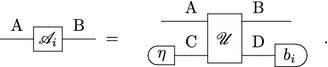
• (7) Reversible dilation of tests Every test $\{\mathscr {A}_i\}_{i\in \mathrm {X}}$ from $\mathrm {A}$ to $\mathrm {B}$ is equivalent to the application of a reversible transformation $\mathscr {U}$ on an enlarged system $\mathrm {A}\mathrm {C}\simeq \mathrm {B}\mathrm {D}$ with $\mathrm {C}$ prepared in a pure state $\eta$, followed by the measurement of an observation-test $\{b_i\}_{i\in \mathrm {X}}$ on system $\mathrm {D}$, as in the following scheme

  

4 Observer, von Neuman Postulate, and Schrödinger Cat

We end the paper with some consideration about the von Neuman postulate and the Schrödinger-cat paradox in the OPT framework.

4.1 The Observer

From a realist point of view the OPT framework is often considered unsatisfying, being inherently dependent on the existence of an “observer”. This is intrinsic to the notions of “observation” and “preparation” that seem to be attached to that of a performing “agent”. Regarding the need of the “observation” as a theoretical ingredient, one can argue that a theory must provide predictions of observations, whether deterministic or probabilistic. Moreover, a theory must consider the existence of incompatible observations among which a definite choice must be made experimentally. On the other hand, the notion of “preparation” is intrinsic to the need of focusing on a portion of reality that is finite both in time and space. This corresponds to setting suitable boundary conditions in space, and both a beginning and an end in time, corresponding to an input-output description. Without setting boundaries and providing an input, the theory would be also required to account for initial conditions. The existence of incompatible observations, on the other hand, is the big conceptual departure of quantum physics from classical physics: the latter has no complementarity, hence no need of choosing the test, every test resorting to a single one: the reading of a point in phase space, or of a bit value in a two-state system. In theories à la Bohm one considers a privileged observation, building up a construction to connect all the other incompatible observations to the privileged one: however, such connections need notions as “position” and “particles” that are mechanical, hence external to a theory of general systems. Indeed, there is no Bohm theory for quantum circuits, whose description can only be given upon resorting to a treatment in terms of the spurious notion of a particle.

4.2 The von Neuman Postulate

In an input-output description where the circuit framework provides a complete physical representation, and assuming causality, the only possible way of connecting theoretically-described portions of reality (i.e., closed circuits) is via an observe-and-prepare test

(2)

where $\{l_i\}_{i\in \mathrm {X}}$ is an observation test, and $\{\omega _i\}_{i\in \mathrm {X}}$ is a set of deterministic states, or more generally a set of preparation tests. This is precisely the “von Neumann process 1”, used in the famous postulate. Thus the von Neumann postulate is just the reconnection of theoretically-described portions of reality in a causal OPT. Entering in some technicalities, one could treat in a similar way also the Lüders rule.

4.3 The Schrödinger Cat

In the OPT framework we can easily understand that the Schrödinger-cat paradox is not exclusive of quantum theory. The paradox consists in the possibility of entangling the state of a microscopic system with that of a macroscopic one—e.g. a radioactive particle that can be decayed or not decayed and a cat that is correspondingly dead or alive, as in the famous ideal experiment by Schrödinger. The paradox indeed simply arises from complementarity between a joint observation-test and any local test. This happens as follows (for simplicity we will assume causality).

Probabilities originate from actualization of potentialities: a priori we know that there is a set of events that can occur; a posteriori we know which event actually occurred. The collection of possible events (the potentialities) depends on which observation-test is chosen, whereas the preparation of the tested systems determines the probability distribution of the outcomes: The state of the systems is nothing but a summary of probability distributions for all possible observation-tests. When we have a composite system to test—e.g. the Schödinger cat along with the radioactive atom—we can perform two kinds of joint observations on the systems that are conceptually radically different: local and nonlocal observations. In the nonlocal observation we make the systems interact, and observe the output of the interaction—a knowingly hard task in the lab. The easy kind of test, instead, is the execution of local observations on systems separately. With the cat working as a measurement apparatus one must have perfect correlation of local observations: dead-cat/decayed-atom, or alive-cat/undecayed-atom. If we were able to perform the nonlocal test we could actually check the existence of entanglement between cat and atom. What happens in the Schrödinger cat thought experiment is that the nonlocal test has no intuitive physical interpretation, since it is incompatible with all possible local observations. The problem would not be cured in a hidden-variable theoretical description à la Bohm. But if one reasons operationally, it is evident that there is no logical paradox, and the described experiment is only highly counterintuitive.

References

Barrett, J.: Information processing in generalized probabilistic theories. Phys. Rev. A 75, 032304 (2007)
Bennett, C.H., Brassard, G.: Quantum cryptography: public key distribution and coin tossing. Theor. Comput. Sci. 560, Part 1(0), 7–11 (2014). Theoretical aspects of quantum cryptography—celebrating 30 years of BB84
Bennett, C.H., Brassard, G., Crepeau, C., Jozsa, R., Peres, A., Wootters, W.K.: Teleporting an unknown quantum state via dual classical and Einstein-Podolsky-Rosen channels. Phys. Rev. Lett. 70, 1895 (1993)
Chiribella, G., D’Ariano, G.M., Perinotti, P.: Probabilistic theories with purification. Phys. Rev. A 81, 062348 (2010)
Chiribella, G., D’Ariano, G.M., Perinotti, P.: Informational derivation of quantum theory. Phys. Rev. A 84, 012311–012350 (2011)
D’ Ariano, G.M.: On the missing axiom of quantum mechanics. AIP Conf. Proc. 810(1), 114–130 (2006)
Fuchs, C.A.: Quantum mechanics as quantum information (and only a little more). http://arxiv.org/abs/quant-ph/0205039
Hardy, L.: Quantum theory from five reasonable axioms. http://arxiv.org/abs/quant-ph/0101012
Shor, P.: Polynomial-time algorithms for prime factorization and discrete logarithms on a quantum computer. SIAM Rev. 41(2), 303–332 (1999)
Wootters, W.K., Zurek, W.H.: A single quantum cannot be cloned. Nature 299, 802 (1982)
Yuen, H.P.: Amplification of quantum states and noiseless photon amplifiers. Phys. Lett. A 113, 405 (1986)
Acknowledgments
This work has been supported in part by the Templeton Foundation under the Project ID# 43796 A Quantum-Digital Universe.
Author information
Authors and Affiliations
Corresponding author
Rights and permissions
About this article
Cite this article
D’Ariano, G.M., Perinotti, P. Quantum Theory is an Information Theory. Found Phys 46, 269–281 (2016). https://doi.org/10.1007/s10701-015-9935-0
Received:
Accepted:
Published:
Issue Date:
DOI: https://doi.org/10.1007/s10701-015-9935-0