
Abstract
Objective
This work was aimed at reducing acoustic noise in diffusion-weighted MR imaging (DWI) that might reach acoustic noise levels of over 100 dB(A) in clinical practice.
Materials and methods
A diffusion-weighted readout-segmented echo-planar imaging (EPI) sequence was optimized for acoustic noise by utilizing small readout segment widths to obtain low gradient slew rates and amplitudes instead of faster k-space coverage. In addition, all other gradients were optimized for low slew rates. Volunteer and patient imaging experiments were conducted to demonstrate the feasibility of the method. Acoustic noise measurements were performed and analyzed for four different DWI measurement protocols at 1.5T and 3T.
Results
An acoustic noise reduction of up to 20 dB(A) was achieved, which corresponds to a fourfold reduction in acoustic perception. The image quality was preserved at the level of a standard single-shot (ss)-EPI sequence, with a 27–54 % increase in scan time.
Conclusions
The diffusion-weighted imaging technique proposed in this study allowed a substantial reduction in the level of acoustic noise compared to standard single-shot diffusion-weighted EPI. This is expected to afford considerably more patient comfort, but a larger study would be necessary to fully characterize the subjective changes in patient experience.
Introduction
Diffusion-weighted MR imaging (DWI) is well established in clinical routine. It is used in stroke imaging [1–5], tumor imaging [6] and exams of white matter disease [7, 8]. Single-shot echo-planar imaging (ss-EPI) with diffusion preparation [9] is currently the sequence of choice in most diffusion-weighted clinical examinations. It is fast, robust and routinely available on commercial MRI scanners. Its limitations include image blurring due to T 2* decay as well as geometric distortions and signal cancellations due to susceptibility changes at tissue interfaces. At higher field strength, these effects become more prominent. Additionally, with increasing image matrix size, stronger distortions occur due to a greater number of echoes and longer echo spacing (ESP). Hence, the maximum achievable resolution is limited.
Another limiting factor is the high acoustic noise level. An ss-EPI readout is particularly demanding for the scanner’s gradient system, since k-space must be covered in the shortest possible time to minimize distortion and susceptibility artifacts. EPI readout and other fast sequences require the combination of high gradient amplitude and rapidly switched polarities. High gradient slew rates lead to mechanical vibrations, creating acoustic pressure waves in the MRI tunnel. In typical examinations, the sound pressure level (SPL) is around 80–105 dB(A) [10]. In experimental scans, the SPL can exceed 130 dB(A) [10–12], depending on sequence and scanner type. Hearing loss may occur at these sound levels [13–15]. For approximate comparison, a sound level of 90 dB(A) is equivalent to that from a pneumatic drill at a distance of 1 m. These high acoustic noise levels are a key reason for patient discomfort and anxiety [16].
Overall, diffusion-weighted (DW) ss-EPI is one of the loudest MRI sequences in clinical routine, due to this high level of gradient activity [12, 17, 18]. Several approaches to reduce acoustic noise have been proposed in recent years. Sequence-based approaches can be implemented on existing systems without expensive hardware modifications. With these methods, the acoustic noise reduction is achieved by optimizing gradient waveforms to minimize the effect of critical components during gradient activity. This is realized, for example, by using sinusoidal-gradient waveforms in RARE (rapid acquisition with relaxation enhancement) and gradient-echo MRI sequences [19, 20] to minimize high acoustic frequencies. A recent study introduced a technique in which the gradient activity is rigorously smoothed using a spline interpolation [21]. Unnecessary gradient activity is removed, while maintaining the net effect of the gradient pulses on the magnetization. This all-purpose algorithm can be applied to a wide range of sequence types. However, for sequences such as ss-EPI, its success is rather limited. This is due to the extended high-slew-rate gradient waveforms in EPI, which are not substitutable. Previous works have investigated reduction of acoustic noise in EPI, but these have been primarily for the purpose of functional MRI (fMRI) [22–25]. With sequence-based optimization methods, mechanical resonance frequencies can be avoided by adapting protocol settings [26] to optimize the frequency spectrum of the applied gradient waveform [27].
The purpose of this work was to develop a technique for acquiring DW images with reduced acoustic noise compared to the standard ss-EPI approach, which was achieved by using DW readout-segmented (rs) echo-planar imaging (rs-EPI) with 2D navigator correction [28]. This is a robust, multi-shot sequence that typically uses a very short ESP in combination with parallel imaging techniques such as generalized autocalibrating partially parallel acquisitions (GRAPPA) [29] to provide clinical DW images with reduced susceptibility and blurring artifacts compared to ss-EPI [30]. However, in this work, the method was primarily employed for the purpose of limiting the level of acoustic noise generated during data acquisition, which was realized by using rs-EPI with reduced gradient slew rates rather than conventional single-shot EPI readouts. We aimed for a tradeoff to deliver an image quality comparable to that of ss-EPI while allowing for a substantial reduction in the level of acoustic noise. Acoustic noise measurements were performed and feasibility was demonstrated in volunteer and patient measurements. In this paper, we compare the acoustic-noise-optimized “quiet DW rs-EPI sequence” to both a “standard DW ss-EPI sequence” and an “unmodified standard DW rs-EPI sequence”.
Materials and methods
The ss-EPI sequence is limited in terms of maximum resolution and suffers from susceptibility artifacts [31]. One method that overcomes these limitations is rs-EPI with 2D navigator correction [28]. In this work, the DW rs-EPI sequence was modified to perform more quietly, and is hereafter termed “quiet-DWI”. Because the generation of acoustic noise is dominated by the EPI readout, the maximum gradient slew rates and amplitudes were reduced to soften the mechanical excitation. In addition, the excitation frequencies were adjusted for non-resonant excitation of the MR system. However, in order to minimize acoustic noise, it is important to optimize all gradient waveforms used by the sequence. The sequence was implemented on a MAGNETOM Aera 1.5T scanner and a MAGNETOM Skyra 3T scanner (Siemens Healthcare, Erlangen, Germany). For all measurements, 20-channel head coil arrays were used.
The following modifications were made to a DW rs-EPI sequence to reduce the acoustic noise load:
-
The maximum slew rates of non-readout gradients were limited to 20 mT/m/ms on all three logical axes. The value is a trade-off between generated acoustic noise and sequence timing. Gradient ramps were merged into each other whenever possible to reduce unnecessary gradient switching. Gradients were preferably run with lower slew rates and higher amplitudes and thus have a triangular shape.
-
The maximum slew rates and amplitudes of the sinusoidal readout gradients were reduced by increasing the ESP from 0.36 to 0.98 ms. The protocols used in this study employed different numbers of readout segments. For a transition from 0.36 to 0.98 ms at 3T and a reduction from 7 to 5 readout segments, the maximum gradient amplitude (slew rate) dropped by a factor of 2.15 (5.97), and for a transition from 0.38 to 0.9 ms at 1.5T while keeping the same number of readout segments, the maximum amplitude (slew rate) dropped by a factor of 2.40 (5.68).
-
Increasing the number of readout segments reduced the amount of acquired data points and thus the size of required gradient moments, slew rates, and amplitudes. For constant data sampling time, the signal-to-noise ratio (SNR) can be increased.
-
Increasing the ESP allowed for a linearly increased sampling dwell time and hence a lower readout bandwidth. The total sampling time was increased, yielding a higher SNR.
-
The data sampling duration was adjusted to allow for blipping of triangular phase-encoding gradients with a fixed slew rate of 15 mT/m/ms between two consecutive data samples.
-
The gradients for traversing k-space (see Fig. 1a) to the start position of the desired segment were placed between the diffusion-preparation gradients (see Fig. 1b). This saves up to 3 ms of TE since gradients do not need to ramp up and down after the radio frequency (RF)-refocusing pulse.
Fig. 1 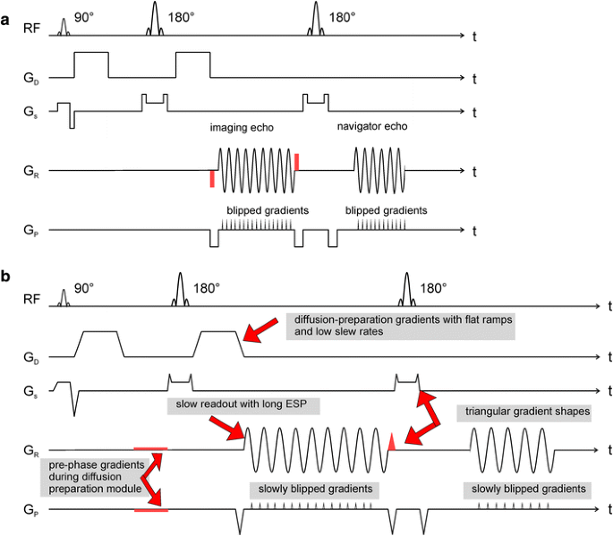
a Sequence diagram for a single readout segment including a 2D navigator echo acquisition. A Stejskal [37] monopolar diffusion preparation is used. The readout segment can be chosen by the gradient moment prior to/after the readout, which is marked in red. b Sequence diagram for the acoustic-noise-optimized readout of a single segment. The major modifications are explained (arrows). The methodology is identical to (a). All non-readout gradients are stretched to reduce the slew rate to the desired level of 20 mT/m/ms. Slower imaging echo readouts are performed. The pre-phase gradients before the EPI readout and the re-phase gradient after the slice selection are integrated into the diffusion preparation module, saving up to 3 ms in TE

The sequence diagram with all applied modifications is shown in Fig. 1b. Doubling or tripling the ESP of the rs-EPI without any further changes leads to longer TEs of 120 ms for the imaging echo and 150 ms for the navigator echo, and the echo train duration (ETD) would then exceed 90 ms. Such a long TE reduces the signal intensity and amplifies T 2 shine-through. The effective TE referenced above corresponds to the time point for the acquisition of the central k-space line which, for the spin-echo-based EPI sequences described below, is coincident with the center of the spin echo. To optimize imaging, the following two adaptions were considered:
-
Application of partial-Fourier (PF) factors of 6/8 and 7/8 in the phase direction: 12.5–25 % of k-space lines are skipped, reducing the SNR as a result of fewer total acquired lines; the k-space center is acquired earlier, thus providing a higher signal, depending on T 2.
-
Increasing the GRAPPA acceleration factor from 2 to 3, thus achieving faster coverage of k-space, which determines the amount of distortion and level of blurring due to T 2* decay, at the cost of SNR
The TE of the 2D navigator echo has less influence on image quality, since its phase information is most relevant.
Protocol settings
The protocols were chosen from those provided by the vendor. The adapted protocols for quiet-DWI where kept comparable. Table 1 summarizes the four protocols used at both field strengths:
-
Standard DW ss-EPI using a default protocol from the vendor as it is used in clinical practice. The ESP and TE chosen were as short as possible with respect to peripheral nerve stimulation constraints.
-
Standard DW rs-EPI using a clinical default protocol from the vendor. The minimum ESP and TE were chosen, which was shorter than those in ss-EPI because of the readout segmentation.
-
Quiet-DWI sequence with PF factor 6/8 and GRAPPA factor 2.
-
Quiet-DWI sequence with PF factor 7/8 and GRAPPA factor 3. ESP and TE longer than those in rs-EPI were chosen for the sake of acoustic noise reduction.
All protocols shared the following parameters: matrix size 192 × 192; field of view (FOV) 230 × 230 mm2; pixel size 1.2 × 1.2 mm2; slice thickness 4 mm at 3T, 5 mm at 1.5T; number of slices, 25; fat suppression prior to every excitation. The b value for diffusion preparation was 1000 s/mm2. Diffusion preparation was applied for three orthogonal directions [32]. The missing PF data were processed using a POCS (projection onto convex sets) [33] reconstruction algorithm. The autocalibration data scan was acquired prior to the measurement with the same readout module. Pre-scan normalization was performed as well as weak k-space filtering. To obtain an estimate for the SNR change in each sequence, the following equation was used:
where avg corresponds to the number of averages, g to the g-factor penalty [31] and BW to the readout bandwidth. For 1.5T (3T), an average T 2 of 80 ms (75 ms) was assumed. Additional gradient echo experiments with a volunteer were performed to obtain g-factor values for GRAPPA factors 2 and 3 for the 3T scanner configuration. The relative SNR
with the highest measured g-factor compared to the ss-EPI protocol is listed in Table 1. In vivo calculation of SNR is challenging, especially when multi-coil arrays and advanced image reconstructions are used. The validity of Eq. (1) was successfully evaluated in phantom experiments.
Acoustic noise measurements
Phantom experiments were performed to measure acoustic noise levels. A PULSE system (Brüel & Kjaer GmbH, Bremen, Germany) with an integrated A-weighting to mimic the sensitivity of the human ear was used to measure acoustic noise on the dB(A) scale. The microphone was moved randomly for 30 s within the bore in front of the head coil. From the temporal sound evolution, the average acoustic noise level and standard deviation were calculated.
In additional phantom experiments, the acoustic noise level dependence on the ESP was determined for the 1.5T and 3T scanners while employing the quiet-DWI sequence with GRAPPA factor 2.
The contributions of slice, phase-encoding, and readout gradients to the total acoustic noise was investigated. As such, the gradients on slice, phase-encoding, and readout axes were selectively disabled for transverse image orientation. The acoustic noise level of seven different combinations of readout, phase-encoding, and slice gradients was measured for the two protocols rs-EPI and quiet-DWI with GRAPPA factor 2 for the 3T scanner.
Sound recordings were taken for all four protocols for the 3T scanner. For the recordings, the calibrated microphone was placed on a small cushion in front of the bore opening in the crosshairs positioning system. The sound levels were saved unnormalized and clipped at a maximum of 110 dB(A) to allow for authentic and comparable playback.
The temporal sound level evolution of the quiet-DWI protocol with PF 6/8 and GRAPPA factor 2 was recorded for the 3T scanner. The sound level evolution was matched with the pulse sequence diagram to analyze the transitions between phase-correction scans, b = 0 s/mm2 scans, and the three orthogonal gradient directions with b = 1000 s/mm2.
In order to differentiate the acoustic noise reduction of the diffusion preparation from the EPI readout, additional experiments were performed at 3T using the quiet-DWI protocol with PF 6/8 and GRAPPA factor 2. First, the maximum diffusion gradient slew rate was set to the default value while a low-slew-rate readout with an ESP of 0.98 ms was performed. Second, the maximum diffusion gradient slew rate was limited to 20 mT/m/ms while a fast readout with ESP of 0.36 ms was performed. The acoustic noise levels were measured and analyzed.
To investigate the impact of a sinusoidal compared to trapezoidal readout as proposed by Schmitter et al. [22], the ss-EPI sequence was modified for sinusoidal readout, and phase-encoding gradients were deactivated to mimic a constant gradient shape. The acoustic noise was measured and compared to the trapezoidal ss-EPI sequence.
In vivo measurements
After obtaining written informed consent, in vivo scans were performed on two healthy volunteers on the 1.5T and 3T scanners. Images were acquired using the following three DW sequences with the above-named protocols: standard ss-EPI, standard rs-EPI, and prototype quiet-DWI.
Two scans were performed on one patient on the 1.5T scanner after written informed consent was obtained. For patient scans, only standard DW ss-EPI images and quiet-DWI images with PF factor 6/8 and GRAPPA factor 2 were acquired. For patient data acquired with the ss-EPI sequence, missing PF data was zero-filled rather than reconstructed by POCS. The images were assessed by three trained radiologists for diagnostic content, image noise and artifacts.
Results
Acoustic noise measurements
The measured dependence of acoustic noise SPL on the readout ESP is shown in Fig. 2. Measurements were not performed for some ESP settings in order to avoid excitation of major system resonance frequencies. For the 1.5T system, a plateau occurred beginning at an ESP of 0.90 ms. For the 3T system, a plateau began at an ESP of 0.98 ms.

Dependence of acoustic noise level SPL on the ESP is shown for a reasonable range of ESPs and the quiet-DWI sequence for the 1.5T and 3T system. Selected ESP values were 0.90 ms for 1.5T and 0.98 ms for 3T. The error bars originate from the standard deviation of the temporal recording. For certain ESP values, resonance frequencies are known, and therefore no measurements were performed. These ESP values span 0.38 to 0.50 ms and 0.66 to 0.78 ms for 1.5T and 0.40 to 0.50 ms and 0.78 to 0.94 ms for 3T
The SPL values recorded during the phantom measurements were as follows: The SPL of the DW ss-EPI sequence was 96.1 ± 0.8 dB(A) for the 1.5T system and 98.6 ± 0.8 dB(A) for the 3T system. The SPL of the standard DW rs-EPI sequence was 100.7 ± 0.7 dB(A) for the 1.5T system and 101.6 ± 0.8 dB(A) for the 3T system. The SPL of the quiet-DWI sequence with PF factor 6/8 and GRAPPA factor 2 was 80.7 ± 0.7 dB(A) for the 1.5T system and 83.4 ± 0.7 dB(A) for the 3T system. For the setting PF factor 7/8 and GRAPPA factor 3, the SPL was 79.9 ± 1.1 dB(A) for the 1.5T system and 82.5 ± 1.0 dB(A) for the 3T system. Acoustic noise reduction in terms of SPL was 19.1–21.7 dB(A) compared to the standard rs-EPI. In terms of acoustic noise pressure, the noise was reduced by a factor of 9.0–12.0. In comparison to the standard ss-EPI, a reduction of 16.1–17.1 dB(A) was achieved. In terms of acoustic noise pressure, the noise was reduced by a factor of 6.4–7.2.
The contribution of different gradient axes on the acoustic noise load is summarized in Table 2. For rs-EPI, acoustic noise is dominated by the readout gradient. Without readout gradients, the acoustic noise drops by 15.5 dB(A); switching off the phase-encoding gradients allows a reduction of another 7.6 dB(A). For the quiet-DWI sequence, the acoustic noise is dominated by both the readout- and phase-encoding gradients. Switching off the readout gradient reduces the acoustic noise by 5.3 dB(A). Switching off the phase-encoding gradient reduces the acoustic noise by 1.7 dB(A). The slice-selection gradient exhibits a sound pressure level of 71.6–78.6 dB(A) and plays the least significant role in acoustic noise generation.
The sound recordings of all four protocols run on the 3T scanner are available in Online Resources 1–4. The sound recording of the ss-EPI protocol can be accessed in Online Resource 1, the rs-EPI protocol recording in Online Resource 2, the recording of the quiet-EPI protocol with GRAPPA factor 2 and PF 6/8 in Online Resource 3, and the recording of the quiet-EPI protocol with GRAPPA factor 3 and PF 7/8 in Online Resource 4. The sound recordings allow the reader to get a better subjective impression of the acoustic noise reduction and the tone of the sequences. Detailed descriptions of changes in sound level and corresponding sequence activity are presented in the “Appendix”.
The temporal sound-level waveform of the quiet-DWI sequence with PF 6/8 and GRAPPA factor 2 showed minor fluctuations. The SPL was reduced by up to 2 dB(A) during phase-correction scans, where no blipped gradients were present. During the subsequent GRAPPA reference scans, phase-encoding blips were noticeable, albeit with reduced intensity due to single-line blipping. During the b = 0 s/mm2 scan, and the three orthogonal diffusion directions with b = 1000 s/mm2, a change in the tone of the sequence (i.e. the subjective acoustic perception) was noticeable. However, no significant variation was observed in terms of SPL. The measured SPL for the protocol with only optimized diffusion gradients was 99.6 dB(A). For the opposite case, when only readout gradients were optimized, an SPL of 90.0 dB(A) was measured.
The acoustic noise level of the ss-EPI sequence was reduced from 98.6 to 93.9 dB(A) after switching from trapezoidal to sinusoidal readout with disabled phase-encoding gradients.
For SNR considerations, the spatially dependent g-factor was determined as g = 1.13–1.81 for GRAPPA factor 2, and g = 1.60–2.56 for GRAPPA factor 3. Hence, changing the GRAPPA factor from 2 to 3 increased the “worst-case” g-factor by 41 %. The estimated “worst-case” SNR changes compared to the ss-EPI protocol are added to Table 1. The “worst-case” SNR change of −23 % obtained for the quiet-DWI protocol with GRAPPA factor 3 is on the order of the SNR of the ss-EPI protocol when only two averages are applied.
In vivo measurements
Example images from healthy volunteers of an axial slice at the level of the lateral ventricles on a 1.5T system are shown in Fig. 3a–h. For the 3T system, example images are shown in Fig. 3i–p. ADC maps and trace-weighted images were also generated. Direct comparisons among ss-EPI, standard rs-EPI, and quiet-DWI with two different GRAPPA factors and PF factors are shown. Depending on the protocol, different levels of geometric distortion next to the frontal sinus can be noted. For both field strengths, the standard DW rs-EPI images are superior to those of the other methods in terms of image quality and amount of artifacts. In comparison, the DW ss-EPI images suffer from susceptibility artifacts. Geometric image distortions next to the frontal sinus occur due to susceptibility differences between air and tissue. Image blurring is less prominent at 1.5T than at 3T. The quiet-DWI images show various levels of geometric image distortion due to susceptibility changes next to the frontal sinus. These distortions are less prominent than those in the ss-EPI images, but more marked than those of the rs-EPI. The same applies to image blurring of quiet-DWI images compared to the ss-EPI and rs-EPI images.

Direct comparison of brain images of two healthy volunteers acquired with ss-EPI, rs-EPI, and quiet-DWI (with PF 6/8, GRAPPA factor 2 and PF 7/8, GRAPPA factor 3) for both 1.5T and 3T field strengths. ADC map (top) and trace-weighted (bottom) images are shown. For 1.5T, the acoustic noise levels are 96.1 dB(A) in (a) and (e), 100.7 dB(A) in (b) and (f), 80.7 dB(A) in (c) and (d), and 79.9 dB(A) in (g) and (h). For 3T, the acoustic noise levels are 98.6 dB(A) in (i) and (m), 101.6 dB(A) in (j) and (n), 83.4 dB(A) in (k) and (l), and 82.5 dB(A) in (o) and (p)
Figure 4 shows data from a typical patient brain examination, with a direct comparison between ss-EPI and quiet-DWI with PF factor 6/8 and GRAPPA factor 2 on a 1.5T system. The patient was in follow-up treatment of a partial middle cerebral artery infarction. The pathology is clearly visible with both methods. In the trace-weighted images, frontal tissue interfaces appear to demonstrate a higher contrast with the quiet-DWI sequence.

Direct comparison of a patient’s brain images at 1.5T between ss-EPI (a and c) and quiet-DWI (b and d) with PF 6/8 and GRAPPA factor 2. Corresponding ADC map (top) and trace-weighted (bottom) images are shown. The acoustic noise levels were 96.1 dB(A) in (a) and (c), and 80.7 dB(A) in (b) and (d)
Discussion
In general, an acoustic noise reduction in MRI sequences can be achieved by reducing the sequence’s gradient slew rates and amplitudes. In EPI, the maximum-gradient performance is typically used, which generates high acoustic noise levels. A pure reduction in the gradient slew rates and amplitudes of the sequence will generate longer ETDs (e.g. 192 ms for an ESP of 2 ms). However, image quality in terms of distortion and image blurring is directly associated with the ETD.
In this work, we have proposed an acoustic-noise-reduced DW imaging sequence based on a DW rs-EPI sequence. In the new approach, an rs-EPI sequence is performed with a longer ESP as necessary to reduce the need for high gradient amplitudes and high slew rates, since the k-space is segmented in readout direction. Different strategies can be employed to maintain fast k-space coverage and short TE at reduced acoustic noise levels in quiet-DWI:
-
Increasing the GRAPPA factor from 2 to 3 reduces the total echo train length, albeit at the expense of lower SNR, mainly due to g-factor effects.
-
Increasing the PF factor reduces the total number of echoes, but also at the expense of lower SNR.
-
Increasing the number of readout segments reduces gradient amplitudes, at the expense of increased measurement time. However, in this case, the SNR is also increased.
In quiet-DWI, the number of RF excitation pulses is higher than in the ss-EPI sequence. A navigator echo allows for phase corrections. However, in the case of non-correctable motion, a reacquisition mode is possible. In general, the advantage of reduced distortion in rs-EPI is traded for acoustic noise reduction. The imaging parameters in quiet-DWI remain the same order of magnitude as in the ss-EPI protocol, with the exception of the beneficial shorter TE and lower readout bandwidth. The smaller readout bandwidth may cause undesired fat–water shift effects. However, in all three sequences, fat saturation pulses are applied prior to excitation to suppress unwanted contributions from fat. While the SPL drops for longer ESP, the imaging parameters would exceed those of the ss-EPI protocol in terms of TE and ETD.
The measurement time of quiet-DWI increases by 27–54 % compared to ss-EPI, depending on the protocol used. Hence, the proposed method is not to be recommended for emergency-case applications. The minimum required measurement time is determined by the number of readout segments. A shorter measurement time may be feasible if only three readout segments are used, but comes at the cost of lower SNR.
Acoustic noise measurements
A recent study [34] showed that acoustic noise is highly dependent on the subject and microphone location within the scanner bore. For this reason, the microphone location in this study was spatially averaged, which is less interpretable as the true exposure to the patients but it is less prone to acoustic resonances within the bore. The averaged value is believed to be a good acoustic noise-specific value. The maximum deviation was 1.9 dB(A), which is acceptable compared to the overall SPL levels.
In addition, the gradients with high amplitude are switched more slowly, and scanner vibrations on the patient table are notably reduced. This is particularly beneficial, since systematic scanner vibrations have been found to cause signal loss in partial-Fourier EPI readouts [35]. However, typical signal-loss artifacts were not observed in this study. We would expect the 16–20 dB(A) reduction in SPL to be considerably more comfortable for the patient, but a larger study would be necessary to fully characterize the subjective changes in patient experience.
To determine the optimal ESP to be used in the sequence, basic initial experiments were performed to characterize the underlying hardware-dependent mechanisms. As demonstrated, the acoustic noise level depends on the frequency-dependent mechanical transfer function which describes the transfer between sequence timing and resulting noise. However, in quiet-DWI, the required slew rates and amplitudes decrease for longer ESPs. The system is excited with less energy, and the frequency dependence of the SPL on ESP decays. For an ESP of 0.36–0.90 ms, the acoustic noise behavior is non-linear due to dependence on resonance frequencies. Starting from an ESP of 0.92–0.94 ms, the acoustic noise level decays linearly, since the frequency of the EPI readout gradients is of minor importance compared to the slew rate of the EPI readout gradients. For ESP longer than 1.0 ms, the SPL remains almost constant, as non-readout gradients start to dominate the acoustic noise level. A further reduction in the slew rate of all gradients may lead to a further reduction of acoustic noise, but would require a longer TE. Reasonable ESP values corresponding to the scanner frequencies with fewer resonances were chosen as a tradeoff. Hence, it must be determined once for every gradient system and bore type. A reasonable ESP of 0.9 ms for 1.5T and 0.98 ms for 3T was found for the two MR systems tested. Different values in the same order of magnitude would be expected for other systems.
The feasibility of DW rs-EPI has been shown for 7T DW imaging [36]. However, because of reduced T 2 and T 2*, shorter TEs are typically used compared to those for 3T. For 7T, the ESP of quiet-DWI might be similar to the ESP of an ss-EPI at 7T in order to match an equal TE. Since gradient moments are reduced substantially due to the readout segmentation, the quiet-DWI approach should allow for a reduction in acoustic noise compared to ss-EPI and rs-EPI. However, the image quality would be on the level of an ss-EPI sequence.
Applying the quiet rs-EPI sequence for the purpose of blood-oxygen-level dependent (BOLD) fMRI with reduced acoustic noise would be an interesting application. However, the application of this multi-shot technique to BOLD fMRI may require changes in acquisition and/or reconstruction strategies, since BOLD fMRI is usually performed in a single-shot mode with high temporal resolution.
The impact of sinusoidal readout gradient shape on the acoustic noise level was measurable. The maximal amplitudes and slew rates remained on the same order of magnitude as on the trapezoidal readout. However, the effect of 4.7 dB(A) was limited in comparison to the proposed method. This can be explained by the required high gradient moments during the EPI readout. In addition, high readout amplitudes such as 30 mT/m occur during readout and may cause peripheral nervous system stimulation. However, the sinusoidal readout gradient shape may be more efficient for smaller matrix sizes. Image reconstruction may be challenging for constant phase-encoding gradients in combination with GRAPPA.
An analysis of the contribution of each gradient axis to the acoustic noise level of the rs-EPI and quiet-DWI sequence was performed. The main contribution originated from the readout gradient, which was confirmed by the second measurement, where no noticeable difference in SPL was noted between b = 0 s/mm2 scans and b = 1000 s/mm2 scans. In all three b = 1000 s/mm2 scans, all three logical gradient directions are run simultaneously, and therefore the deviation in SPL is relatively low, since all gradients are employed during all three diffusion direction scans. The loud EPI readout was successfully addressed in quiet-DWI by increasing the ESP. Measurements with GRAPPA factor 2 were up to 0.9 dB(A) louder than those with GRAPPA factor 3, which was due to the higher number of noise-generating EPI echoes in GRAPPA factor 2 imaging. As shown in the subsequent experiments, the second-loudest contribution originated from the diffusion-preparation gradients, which could be addressed by reducing the slew rate. In addition, the acoustic noise contribution of the phase-encoding gradient could be reduced to less than 80 dB(A). The slice selection gradients could benefit from gradient shape optimization. Overall, the experiments showed that acoustic noise reduction requires simultaneous optimization of both the diffusion-preparation gradients and EPI readout.
In vivo measurements
Both in vivo volunteer experiments and patient measurements were performed to test and compare the quiet-DWI sequence with standard clinical sequences. Images of healthy volunteers acquired with the proposed DWI methods are shown in Fig. 3. The images were assessed by three trained radiologists. All acquired images provided identical diagnostic information and sufficient image quality. Image quality should be evaluated in further clinical studies.
Conclusions
Diffusion-weighted imaging with an EPI readout typically exposes patients to high acoustic noise. This paper describes a software-based method for significantly reducing acoustic noise in DWI without the need for hardware modification. For this purpose, the maximum gradient slew rates of a DW rs-EPI sequence were reduced by over 82 %. The image quality was addressed in healthy volunteer and patient measurements at 1.5T and 3T, and were maintained at the level of a standard ss-EPI while requiring an increase of 27–54 % in scan time. The results shown here were achieved at around 79–83 dB(A). A significant acoustic noise reduction of 84–92 % in sound pressure was achieved. This corresponds to a twofold to fourfold reduction in acoustic perception. In conclusion, DW EPI measurements were successfully performed with a reduction in acoustic noise levels.
References
Moseley ME, Kucharczyk J, Mintorovitch J, Cohen Y, Kurhanewicz J, Derugin N, Asgari H, Norman D (1990) Diffusion-weighted MR imaging of acute stroke: correlation with T2-weighted and magnetic susceptibility-enhanced MR imaging in cats. AJNR Am J Neuroradiol 11:423–429
Warach S, Chien D, Li W, Ronthal M, Edelman RR (1992) Fast magnetic resonance diffusion-weighted imaging of acute human stroke. Neurology 42:1717–1723
Warach S, Gaa J, Siewert B, Wielopolski P, Edelman RR (1995) Acute human stroke studied by whole brain echo planar diffusion-weighted magnetic resonance imaging. Ann Neurol 37:231–241
van Everdingen KJ, van der Grond J, Kappelle LJ, Ramos LM, Mali WP (1998) Diffusion-weighted magnetic resonance imaging in acute stroke. Stroke 29:1783–1790
Wu O, Koroshetz WJ, Ostergaard L, Buonanno FS, Copen WA, Gonzalez RG, Rordorf G, Rosen BR, Schwamm LH, Weisskoff RM, Sorensen AG (2001) Predicting tissue outcome in acute human cerebral ischemia using combined diffusion- and perfusion-weighted MR imaging. Stroke 32:933–942
Kono K, Inoue Y, Nakayama K, Shakudo M, Morino M, Ohata K, Wakasa K, Yamada R (2001) The role of diffusion-weighted imaging in patients with brain tumors. AJNR Am J Neuroradiol 22:1081–1088
Bozzali M, Falini A, Franceschi M, Cercignani M, Zuffi M, Scotti G, Comi G, Filippi M (2002) White matter damage in Alzheimer’s disease assessed in vivo using diffusion tensor magnetic resonance imaging. J Neurol Neurosurg Psychiatry 72:742–746
Rose SE, Chen F, Chalk JB, Zelaya FO, Strugnell WE, Benson M, Semple J, Doddrell DM (2000) Loss of connectivity in Alzheimer’s disease: an evaluation of white matter tract integrity with colour coded MR diffusion tensor imaging. J Neurol Neurosurg Psychiatry 69:528–530
Turner R, Le Bihan D, Maier J, Vavrek R, Hedges LK, Pekar J (1990) Echo-planar imaging of intravoxel incoherent motion. Radiology 177:407–414
Moelker A, Maas RA, Vogel MW, Ouhlous M, Pattynama PM (2005) Importance of bone-conducted sound transmission on patient hearing in the MR scanner. J Magn Reson Imaging 22:163–169
Counter SA, Olofsson A, Borg E, Bjelke B, Haggstrom A, Grahn HF (2000) Analysis of magnetic resonance imaging acoustic noise generated by a 4.7 T experimental system. Acta Otolaryngol 120:739–743
Foster JR, Hall DA, Summerfield AQ, Palmer AR, Bowtell RW (2000) Sound-level measurements and calculations of safe noise dosage during EPI at 3 T. J Magn Reson Imaging 12:157–163
Committee on Environmental Health (1997) Noise: a hazard for the fetus and newborn. Pediatrics 100:724–727
Rabinowitz PM (2000) Noise-induced hearing loss. Am Fam Physician 61:2759–2760
Clark WW (1992) Hearing: the effects of noise. Otolaryngol Head Neck Surg 106:669–676
Quirk ME, Letendre AJ, Ciottone RA, Lingley JF (1989) Anxiety in patients undergoing MR imaging. Radiology 170:463–466
McJury M, Shellock FG (2000) Auditory noise associated with MR procedures: a review. J Magn Reson Imaging 12:37–45
Mansfield P, Glover PM, Beaumont J (1998) Sound generation in gradient coil structures for MRI. Magn Reson Med 39:539–550
Hennel F, Girard F, Loenneker T (1999) “Silent” MRI with soft gradient pulses. Magn Reson Med 42:6–10
Hennel F (2001) Fast spin echo and fast gradient echo MRI with low acoustic noise. J Magn Reson Imaging 13:960–966
Heismann B, Ott M, Grodzki D (2015) Sequence-based acoustic noise reduction of clinical MRI scans. Magn Reson Med 73:1104–1109. doi:10.1002/mrm.25229
Schmitter S, Diesch E, Amann M, Kroll A, Moayer M, Schad LR (2008) Silent echo-planar imaging for auditory FMRI. Magn Reson Mater Phy 21:317–325
Miyati T, Banno T, Fujita H, Mase M, Narita H, Imazawa M, Sanada S, Koshida K, Kasuga T (2001) Characteristics of acoustic noise in echo-planar imaging. Front Med Biol Eng 10:345–356
Zapp J, Schmitter S, Schad LR (2012) Sinusoidal echo-planar imaging with parallel acquisition technique for reduced acoustic noise in auditory fMRI. J Magn Reson Imaging 36:581–588
Tomasi DG, Ernst T (2003) Echo planar imaging at 4 Tesla with minimum acoustic noise. J Magn Reson Imaging 18:128–130
Baker MA (2013) Reduction of MRI acoustic noise achieved by manipulation of scan parameters—a study using veterinary MR sequences. Radiography 19:11–16
Blecher WD (2009) The Hilbert–Moore sequence acoustic noise optimized MR imaging. Dissertation, University of Mannheim, Germany
Porter DA, Heidemann RM (2009) High resolution diffusion-weighted imaging using readout-segmented echo-planar imaging, parallel imaging and a two-dimensional navigator-based reacquisition. Magn Reson Med 62:468–475
Griswold MA, Jakob PM, Heidemann RM, Nittka M, Jellus V, Wang J, Kiefer B, Haase A (2002) Generalized autocalibrating partially parallel acquisitions (GRAPPA). Magn Reson Med 47:1202–1210
Morelli J, Porter D, Ai F, Gerdes C, Saettele M, Feiweier T, Padua A, Dix J, Marra M, Rangaswamy R, Runge V (2013) Clinical evaluation of single-shot and readout-segmented diffusion-weighted imaging in stroke patients at 3 T. Acta Radiol 54:299–306
Pruessmann KP, Weiger M, Scheidegger MB, Boesiger P (1999) SENSE: sensitivity encoding for fast MRI. Magn Reson Med 42:952–962
Sorensen AG, Weisskoff RM, Reese TR, Rosen BR (1995) Optimisation of diffusion-weighted MR imaging for evaluation of acute stroke. In: Proceedings of the 3rd scientific meeting, International Society for Magnetic Resonance in Medicine, Nice, p. 1383
Cuppen J, van Est A (1987) Reducing MR imaging time by one-sided reconstruction. Magn Reson Imaging 5:526–527
Segbers M, Rizzo Sierra CV, Duifhuis H, Hoogduin JM (2010) Shaping and timing gradient pulses to reduce MRI acoustic noise. Magn Reson Med 64:546–553
Gallichan D, Scholz J, Bartsch A, Behrens TE, Robson MD, Miller KL (2010) Addressing a systematic vibration artifact in diffusion-weighted MRI. Hum Brain Mapp 31:193–202
Heidemann RM, Porter DA, Anwander A, Feiweier T, Heberlein K, Knosche TR, Turner R (2010) Diffusion imaging in humans at 7T using readout-segmented EPI and GRAPPA. Magn Reson Med 64:9–14
Stejskal E, Tanner J (1965) Spin diffusion measurements: spin echoes in the presence of a time-dependent field gradient. J Chem Phys 42:288–292
Acknowledgments
The authors thank Anagha Deshmane for assistance in proofreading of the manuscript.
Conflict of interest
Drs. Grodzki and Heismann are employees of Siemens Healthcare. All other authors declare that they have no conflict of interest.
Ethical standard
Informed consent was obtained from all volunteers and patients included in the study.
Author information
Authors and Affiliations
Corresponding author
Electronic supplementary material
Below is the link to the electronic supplementary material.
Appendix
Appendix
The scans in the OR have the following temporal sequence activity:
OR1 (ss-EPI): dummy scans (1–14 s), ACS scans (14–20 s), interleaved averages of b = 0 s/mm2 scans and three b = 1000 s/mm2 scans (20–102 s).
OR2 (rs-EPI) and OR4 (quiet-DWI GRAPPA factor 3) are conceptually identical: dummy scans (1–5 s), phase-correction scans (5–10 s), ACS scans (10–15 s), b = 0 s/mm2 scans (15–50 s) and three b = 1000 s/mm2 scans (50–85 s, 85–120 s, 120–155 s).
OR3 (quiet-DWI GRAPPA factor 2): dummy scans (1–6 s), phase-correction scans (6–12 s), ACS scans (12–18 s), b = 0 s/mm2 scans (18–48 s) and three b = 1000 s/mm2 scans (48–76 s, 76–106 s, 106–136 s).
Rights and permissions
About this article

Cite this article
Ott, M., Blaimer, M., Grodzki, D.M. et al. Acoustic-noise-optimized diffusion-weighted imaging. Magn Reson Mater Phy 28, 511–521 (2015). https://doi.org/10.1007/s10334-015-0492-5
Received:
Revised:
Accepted:
Published:
Issue Date:
DOI: https://doi.org/10.1007/s10334-015-0492-5