From a quantum theory to a classical one

Abstract

We present and discuss a formal approach for describing the quantum to classical crossover based on the group-theoretic construction of generalized coherent states. The method was originally introduced by Yaffe (Rev Mod Phys 54:407, 1982) in 1982 for tackling large-N quantum field theories and has been recently used for studying open quantum systems whose environment, while becoming macroscopic, may or may not display a classical behaviour (Liuzzo-Scorpo et al. in EPL (Europhys Lett) 111(4):40008, 2015; Rossi et al. in Phys Rev A 96:032116, 2017; Foti et al. in Quantum 3:179, 2019; Coppo in Schwarzschild black holes as macroscopic quantum systems, Università degli studi di Firenze, Florence, 2019). Referring to these recent developments, in this paper we provide the essential elements of Yaffe’s approach in the framework of standard quantum mechanics, so as to clarify how the approach can be used without referring to quantum field theory. Moreover, we address the role played by a possible global symmetry in making the large-N limit of the original quantum theory to flow into a formally well-defined classical theory, and we specifically consider the quantum-to-classical crossover of angular momentum. We also give details of a paradigmatic example, namely that of N free one-dimensional spinless particles. Finally, we discuss upon the foundational requirement that any classical description should ultimately be derived from an underlying quantum theory, that, however, is not, and should never be confused with, the one obtained via some quantization procedure of the classical description itself.

1 Introduction

Progresses in quantum technologies have recently made necessary to deeply understand the relation between macroscopic objects that behave according to a classical theory, and the quantum world of microscopic systems, in order to find the best strategies for using, interacting, and exerting control upon small and fragile quantum devices. Key to this understanding is a formal description of the so-called quantum to classical crossover, implying the possibility of connecting the geometrical structure of classical physics with the algebraic one featured by quantum mechanics. Some powerful tools in this framework can be found in the literature relative to the so-called large-N quantum field theories: although they cannot be straightforwardly used in different settings, such as those typically arising in the analysis of open quantum systems, where the system undergoing the above crossover is just the big partner of a small quantum object, they are versatile enough to be adapted and turn very useful even in these frameworks. In particular, the way Yaffe (1982) in 1982 tackled some large-N quantum field theories has demonstrated very powerful and has been recently used for studying open quantum systems whose environment, while becoming macroscopic, may or may not display a classical behaviour (Liuzzo-Scorpo et al. 2015; Rossi et al. 2017; Foti et al. 2019; Coppo 2019). In this paper, after providing the essential elements of Yaffe’s approach in the framework of standard quantum mechanics, we elaborate upon the role of the global symmetry, whose presence in the original quantum theory turns out to be a primary requirement to ensure that its large-N limit is a well-defined classical theory. The practical implementation of the general abstract approach is described in detail for two specific examples: the quantum-to-classical crossover of angular momentum and the deduction of the classical limit of a system made of N free one-dimensional spinless particles. The structure of the paper is as follows: in Sect. 2 we introduce the generalized coherent states (GCS, which are essential in Yaffe’s procedure) via the group-theoretic approach, independently developed by Gilmore (1972) and Perelomov (1972) in 1972. Following Zhang et al. (1990) we describe the algebraic procedure to construct GCS starting from the knowledge of the dynamical group of the system. In particular, we show how to construct GCS for systems associated with one of the two real forms of the Lie group $SL(2,{\mathbb {C}})$, namely the non-compact one SU(1, 1), whose proper GCS are the so-called pseudo-spin coherent states (PCS). In Sect. 3 we identify the conditions ensuring that a quantum theory has a well-defined classical limit, while in Sect. 4 we consider a specific case to show that such limit can be obtained by increasing the number of degrees of freedom N of the original quantum theory, i.e. when the system it describes becomes macroscopic, as briefly discussed in the last concluding section.

2 Generalized coherent states

Any quantum theory ${\mathcal {Q}}$ can be defined in terms of an algebra, possibly a Lie algebra ${\mathfrak {g}}$, and a Hilbert space ${\mathcal {H}}$, which is the carrier space of an irreducible representation of ${\mathfrak {g}}$. All the physically relevant operators on ${\mathcal {H}}$, except for the propagators, are elements of such representation. On the other hand, according to the evolution postulate of quantum mechanics, the propagators of ${\mathcal {Q}}$ are elements of a unitary irreducible representation of the Lie group ${\mathcal {G}}$ obtained from ${\mathfrak {g}}$ via a Lie exponential map, for that ${\mathcal {G}}$ is called “dynamical group”. In what follows, for the sake of a lighter presentation, we will most often identify algebras and groups with their respective representations.

Let us now consider a generic quantum system described by a theory ${\mathcal {Q}}$ such that its Hamiltonian ${\hat{H}}$ belongs to ${\mathfrak {g}}$:

$$\begin{aligned} {\hat{H}}{=}H({\hat{g}}_i),~\text{ where }~~{\hat{g}}_i \in {{\mathfrak {g}}},~\text{ and }~~[{\hat{g}}_i,{\hat{g}}_j]= c_{ij}^k {\hat{g}}_k. \end{aligned}$$

(1)

If we limit our analysis to semisimple Lie algebras (or any algebra admitting a Cartan decomposition), the Cartan basis {$\hat{D_i},{\hat{E}}_\alpha ,{\hat{E}}_{-\alpha }$} is defined, with

$$\begin{aligned}&[{\hat{D}}_i,{\hat{D}}_j]=0,~[{\hat{D}}_i,{\hat{E}}_\alpha ] =\alpha _i {\hat{E}}_\alpha ,\\&[{\hat{E}}_\alpha ,{\hat{E}}_{-\alpha }]=\alpha _i {\hat{D}}^i,~[{\hat{E}}_\alpha ,{\hat{E}}_\beta ]=C_{\alpha \beta } {\hat{E}}_{\alpha +\beta }, \end{aligned}$$

${\hat{D}}_i$ Hermitian (${\hat{D}}_i^\dagger ={\hat{D}}_i$), and ${\hat{E}}_\alpha$ such that ${\hat{E}}_\alpha ^\dagger ={\hat{E}}_{-\alpha }$. The elements ${\hat{D}}_i({\hat{E}}_\alpha )$ are dubbed diagonal(shift) operators.

Once a normalized reference state in ${\mathcal {H}}$ is chosen, usually so as to be both an eigenstate of diagonal operators and a maximal weight state, i.e.

(2)

one can identify the subgroup ${\mathcal {F}}\subset {\mathcal {G}}$ that leaves invariant up to a phase factor, i.e. ; this subgroup is called stabilizer of ${\mathcal {G}}$ with respect to . Finally, referring to the coset ${\mathcal {G}}/{\mathcal {F}}$, the generalized coherent states are defined by:

(3)

where

$$\begin{aligned} {\hat{G}}={\hat{\varOmega }} {\hat{F}} \;\;\; {\hat{G}} \in {\mathcal {G}},\;{\hat{F}}\in {\mathcal {F}}, \; {\hat{\varOmega }}\in {\mathcal {G}}/{\mathcal {F}}. \end{aligned}$$

We notice that GCS are in one-to-one correspondence with the elements ${\hat{\varOmega }}$ of ${\mathcal {G}}/{\mathcal {F}}$.

2.1 Differential structure of ${\mathcal {G}}/{\mathcal {F}}$

According to the “quotient manifold theorem” (Lee 2012), the coset ${\mathcal {G}}/{\mathcal {F}}$ can be associated with a complex manifold ${\mathcal {M}}$ whose points $\varOmega$ are in one-to-one correspondence with operators ${\hat{\varOmega }}$ in ${\mathcal {G}}/{\mathcal {F}}$, and hence with the states . Since the algebra ${\mathfrak {g}}$ is semisimple, it satisfies the Cartan decomposition in the form ${\mathfrak {g}}={\mathfrak {f}}\oplus {\mathfrak {p}}$, where ${\mathfrak {f}}$ is the algebra of ${\mathcal {F}}$ and ${\mathfrak {p}} = \xi ^\beta {\hat{E}}_\beta -{\xi ^\beta }^* {\hat{E}}_{-\beta }$ is its orthogonal complement; therefore, we can use the coordinates $\left\{ \xi ^\beta , {\xi ^\beta }^*\right\}$ to write

$$\begin{aligned} {\hat{\varOmega }}=\mathrm {e}^{\left( \xi ^\beta {\hat{E}}_\beta -{\xi ^\beta }^* {\hat{E}}_{-\beta }\right) },\qquad \xi _{\beta }\in {\mathbb {C}}. \end{aligned}$$

(4)

One can use other coordinate systems such as, dropping the $\beta$-index for the sake of a lighter notation,

(5)

or the one yielding a complex projective representation,

$$\begin{aligned} {\left\{ \begin{array}{ll} \tau =\zeta (1-\zeta ^\dagger \zeta )^{-\frac{1}{2}}&{}\quad \text{ if } {\mathcal {M}} \text{ is } \text{ compact },\\ \tau =\zeta (1+\zeta ^\dagger \zeta )^{-\frac{1}{2}}&{}\quad \text{ if } {\mathcal {M}} \text{ is } \text{ not } \text{ compact }. \end{array}\right. } \end{aligned}$$

(6)

2.2 Metric and measure

It can be demonstrated (Hua 1963) that ${\mathcal {M}}$ is endowed with a natural metric that can be expressed in the $\tau$ coordinates as

(7)

where is a non-normalized GCS. This allows one to get information upon the manifold ${\mathcal {M}}$. Through $\mathrm{d}s^2$ one can define a canonical volume form on ${\mathcal {M}}$, i.e. a measure

$$\begin{aligned} \mathrm{d}\mu (\varOmega )= \text{ const } \times \det (g) \prod _{\alpha } \mathrm{d}\tau ^\alpha \mathrm{d}{\tau ^\alpha }^*. \end{aligned}$$

(8)

2.3 Overcompleteness of coherent states

Using $\mathrm{d}\mu (\varOmega )$, GCS are demonstrated to form an overcomplete set of states on ${\mathcal {H}}$, providing a continuous resolution of the identity, i.e.

(9)

The prefix “over” in the adjective “overcomplete” indicates that coherent states are “a lot”: in fact, despite being normalized, , $\forall {\hat{G}}\in {\mathcal {G}}$, they are not orthogonal,

(10)

$\forall \;{\hat{G}},{\hat{G}}',{\hat{G}}'' \in {\mathcal {G}}$, and ${\hat{\varOmega }},{\hat{\varOmega }}'\in {\mathcal {G}}/{\mathcal {F}}$.

2.4 Symplectic structure

${\mathcal {M}}$ is equipped with a symplectic structure that allows one to identify it as a phase space, possibly the one proper to the classical system into which the original quantum system flows when the classical limit is rigorously performed. The symplectic form on ${\mathcal {M}}$ has the coordinate representation

$$\begin{aligned} \omega =-\,i\;\sum _{\alpha \beta }g_{\alpha \beta }\,\mathrm{d}\tau ^\alpha \wedge \mathrm{d}{\tau ^\beta }^*, \end{aligned}$$

(11)

and it is used to define the Poisson brackets

$$\begin{aligned} \left\{ f,g\right\} _{PB}:=i\;\sum _{\alpha \beta }g^{\alpha \beta }\left( \frac{\partial f}{\partial \tau ^\alpha } \frac{\partial g}{\partial {\tau ^\beta }^*} - \frac{\partial g}{\partial \tau ^\alpha } \frac{\partial f}{\partial {\tau ^\beta }^*}\right) . \end{aligned}$$

(12)

Switching to the $\zeta$ coordinates and defining w and v via

$$\begin{aligned} \zeta _\beta =\frac{1}{\sqrt{2}}\left( w_\beta -iv_\beta \right) ,\quad \zeta _\beta ^*=\frac{1}{\sqrt{2}}\left( w_\beta +iv_\beta \right) , \end{aligned}$$

(13)

one obtains the Poisson brackets in the standard form,

$$\begin{aligned} \left\{ f,g\right\} _{PB}=\sum _{\alpha }\left( \frac{\partial f}{\partial v^\alpha } \frac{\partial g}{\partial w^\alpha } - \frac{\partial g}{\partial v^\alpha } \frac{\partial f}{\partial w^\alpha }\right) . \end{aligned}$$

(14)

2.5 Pseudo-spin coherent states

We end this section by giving an explicit example of GCS construction, namely those relative to the group SU(1, 1).¹ Its generators are the set $\{{\hat{K}}_0,{\hat{K}}_1,{\hat{K}}_2\}$ which spans the ${\mathfrak {su}}(1,1)$ algebra

$$\begin{aligned}{}[{\hat{K}}_\alpha ,{\hat{K}}_\beta ]=i\epsilon _{\alpha \beta \gamma }{\hat{K}}^\gamma , \end{aligned}$$

(15)

where the indices $\alpha ,\beta ,\gamma \in \{0,1,2\}$ are raised and lowered with the three-dimensional Minkowski metric $\eta _{\alpha \beta }=\text{ diag }\{-1,1,1\}$. The Hilbert space of the system is a unitary irreducible representation of ${\mathfrak {su}}(1,1)$, which is identified by the so-called Bargmann index k:

(16)

where are the simultaneous eigenstates of ${\hat{K}}_0$ and of the Casimir operator ${\hat{K}}^2=-\,{\hat{K}}_\alpha {\hat{K}}^\alpha$ such that

(17)

The unitary irreducible representations of SU(1, 1) (that are infinite-dimensional since the group is not compact) have been firstly discussed by Bargmann (1947) as incidental to his discussion of the Lorentz group. One can find a consolidated review in Biedenharn et al. (1965). In this paper, we will only refer to the representations of the group $SO(1,2)=SU(1,1)/{\mathbb {Z}}_2$, obtained by Barut and Fronsdal (1965).

To construct GCS, we need a reference state. Given the index-k representation, we choose the lowest-weight state, i.e. , and we identify the stabilizer subgroup ${\mathcal {F}}$ by

(18)

and hence ${\mathcal {F}}=U(1)$. We can now consider the coset SU(1, 1)/U(1) to define the pseudo-spin coherent states (PCS)

(19)

where ${\hat{\varOmega }}$ can be parameterized as:

$$\begin{aligned} {\hat{\varOmega }}=\mathrm {e}^{\xi {\hat{K}}_+ - \xi ^* {\hat{K}}_-} \end{aligned}$$

(20)

with ${\hat{K}}_\pm ={\hat{K}}_1 \pm i {\hat{K}}_2$ shift operators satisfying $[{\hat{K}}_+,{\hat{K}}_-]=-\,2{\hat{K}}_0$, $[{\hat{K}}_0,{\hat{K}}_\pm ]=\pm \, {\hat{K}}_\pm$. Points $\varOmega$ on the manifold associated with the coset SU(1, 1)/U(1) can be identified by the complex coordinates $(\xi ,\xi ^*)$; this allows one to express ${\hat{\varOmega }}$, using the standard $(2\times 2)$ matrix representation²

$$\begin{aligned} {\hat{K}}_+=\begin{bmatrix} 0 &{} \quad i\\ 0 &{} \quad 0 \end{bmatrix}\quad {\hat{K}}_-=\begin{bmatrix} 0 &{}\quad 0\\ i &{}\quad 0 \end{bmatrix}\quad {\hat{K}}_0=\begin{bmatrix} \frac{1}{2} &{} \quad 0 \\ 0 &{} \quad -\frac{1}{2} \end{bmatrix}, \end{aligned}$$

(21)

by means of the matrix (Zhang et al. 1990)

$$\begin{aligned} \begin{bmatrix} \sqrt{1+\zeta \zeta ^*} &{} \quad \zeta \\ \zeta ^* &{} \quad \sqrt{1+\zeta \zeta ^*} \end{bmatrix}, \end{aligned}$$

(22)

with $-i\zeta$ defined by Eq. (5).³ Introducing “polar” coordinates $(\rho ,\phi )\in {\mathbb {R}}\times [0,2\pi ]$ via

$$\begin{aligned} i\xi =\frac{\rho }{2}\mathrm {e}^{-i\phi } \end{aligned}$$

(23)

Equations (5) and (6) define the $\zeta$- and $\tau$-coordinates as

$$\begin{aligned} \zeta =\sinh {\frac{\rho }{2}}\mathrm {e}^{-i\phi },\;\;\tau =\tanh {\frac{\rho }{2}}\mathrm {e}^{-i\phi }. \end{aligned}$$

(24)

Equation (20) can be written (Perelomov 1985) in the $\tau$-coordinates

$$\begin{aligned} {\hat{\varOmega }}=(1-|\tau |^2)^k\mathrm {e}^{\tau {\hat{K}}_+} \end{aligned}$$

(25)

so that the natural metric defined in Eq. (7) emerges via

(26)

as

$$\begin{aligned} \mathrm{d}s^2=\frac{2k}{(1-|\tau |^2)^2}\mathrm{d}\tau \mathrm{d}{\tau }^*=\frac{k}{2}(d^2\rho +\sinh ^2{\rho }\,d^2\phi ), \end{aligned}$$

(27)

where is a non-normalized PCS. Moreover, it is possible to show (Perelomov 1985) that the completeness relation (9) is verified for any $k>1/2$ in the form

(28)

The manifold associated with SU(1, 1)/U(1) is called “Bloch” pseudo-sphere $PS^2$ [see, for instance, Chap. 1 of Coppo (2019) for further details].

3 From a quantum theory to a classical one

In this section, following Yaffe (1982), we show how a large-N limit of a quantum theory can formally define a classical dynamics. Let us first specify what makes a theory recognizable as a quantum or a classical one: as mentioned in Sect. 2, a quantum theory${\mathcal {Q}}$ is defined by:

• a Lie Algebra ${\mathfrak {g}}$,

• a Hilbert space ${\mathcal {H}}$ that carries an irreducible representation of ${\mathfrak {g}}$,

• a Hamiltonian operator ${\hat{H}}\in {\mathfrak {g}}$.

A classical theory${\mathcal {C}}$ is instead determined by⁴:

• a manifold ${\mathcal {M}}$,

• a symplectic form on ${\mathcal {M}}$, which defines Poisson brackets,

• a Hamiltonian function $h_{cl}:{\mathcal {M}}\rightarrow {\mathbb {R}}$.

After the above definitions, one can describe a general procedure for realizing a so-called quantum-to-classical crossover, which is a formal relation between quantum and classical theories, describing how the first can naturally flow into the latter, possibly when some “quanticity parameter” $\chi \in {\mathbb {R}}^+$ tends to zero. The limit $\chi \rightarrow 0$ is dubbed “classical limit” and, in order to exist, certain conditions must be fulfilled that isolate the minimal structure that the starting quantum theory should possess. These conditions are satisfied by a large class of quantum theories, namely the Large-N quantum theories that feature a global symmetry. If this is the case, $\chi$ is a decreasing function of the number N of degrees of freedom, and $\chi \rightarrow 0$ when $N\rightarrow \infty$. This reveals that many variables, provided with a global symmetry, lie behind any quantum-to-classical crossover.

3.1 When does a quantum theory have a classical limit?

Consider a quantum theory ${\mathcal {Q}}_\chi$ defined by the Lie algebra ${\mathfrak {g}}$, the Hilbert space ${\mathcal {H}}_\chi$ and the Hamiltonian ${\hat{H}}_\chi$. Be such theory characterized by some parameter $\chi$ which is assumed to take positive real values, including the limiting $\chi =0$ one. Once identified the dynamical group ${\mathcal {G}}$ of the theory via a Lie exponential map on ${\mathfrak {g}}$, and its irreducible unitary representation⁵${\mathcal {G}}_\chi$ on ${\mathcal {H}}_\chi$, we can construct the GCS . They will be in one-to-one correspondence with the points $\varOmega _\chi$ of the manifold ${\mathcal {M}}_\chi$ associated with the coset ${\mathcal {G}}/{\mathcal {F}}_\chi$, where ${\mathcal {F}}_\chi$ is the stabilizer with respect to a reference state . For any operator ${\hat{A}}$ acting on ${\mathcal {H}}_\chi$, one can define the symbol $A(\varOmega _\chi )$ by

(29)

As pointed out in Yaffe (1982), in order to have some control over the limit $\chi \rightarrow 0$, suppose that it is possible to arrange the set of GCS in the equivalence classes

(30)

obtained from the equivalence relation

(31)

where, in order to ensure that the limit is well defined, ${\mathcal {K}}$ is a restricted set of operators satisfying

(32)

operators in ${\mathcal {K}}$ will be called classical operators. Since the symbols of classical operators upon GCS that belong to a same class are equal, according to Eq. (31), we will use the notation:

(33)

It can be demonstrated (Yaffe 1982) that, in order for the theory ${\mathcal {Q}}_\chi$ to have a $\chi \rightarrow 0$ limit that corresponds to a classical theory, the following conditions must hold:

• 1. Irreducibility of ${\mathcal {G}}_\chi$

  As mentioned above, each representation ${\mathcal {G}}_\chi$ of the dynamical group acts irreducibly on the corresponding Hilbert space ${\mathcal {H}}_\chi$. This requirement assures that for each $\chi$ the quantum theory is well defined. Using the Schur’s lemma and the invariance of the measure on the coset ${\mathcal {G}}/{\mathcal {F}}_\chi$, this assumption implies Eq. (9), i.e.

  

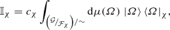  (34)

  where $c_\chi$ is a constant depending on the normalization of the group measure and must be computed explicitly. Notice that the measure $\mathrm{d}\mu (\varOmega )$ does not depend on $\chi$ and hence remains the same as $\chi \rightarrow 0$.

• 2. Uniqueness of the “Zero” operator

  The zero operator ${\hat{Z}}$ is the only one for which $Z_\chi (\varOmega )=0\quad \forall \varOmega \in {\mathcal {M}}_\chi /\sim$. As a consequence, two different operators cannot have the same symbol, implying that any operator can be uniquely recovered from its expectation value on GCS, i.e. from its symbols.

• 3. Exponential decrease in inequivalent coherent states overlaps

  The overlap between classically inequivalent GCS exponentially decreases as $\chi \rightarrow 0$, i.e.

  

  (35)

  where $\exists \lim _{\chi \rightarrow 0}{\varDelta (\varOmega ,\varOmega ')_\chi }$$\forall \varOmega ,\varOmega '\in {\mathcal {M}}_\chi /\sim$ and

  

  The result is that, when $\chi \rightarrow 0$ inequivalent coherent states become orthogonal, i.e. distinguishable. As a consequence, the factorization

  $$\begin{aligned} \lim _{\chi \rightarrow 0}[(AB)_\chi (\varOmega )- A_\chi (\varOmega )B_\chi (\varOmega )]=0 \end{aligned}$$

  (36)

  holds for any pair ${\hat{A}}$ and ${\hat{B}}$ of classical operators.

• 4. Classical limit of the Hamiltonian

  The operator $\chi {\hat{H}}_\chi$ is a classical operator. This ensures that the coupling constants in the Hamiltonian are scaled in a manner that maintains sensible dynamics as $\chi \rightarrow 0$, so as to define a meaningful classical limit.

If the hypotheses 1–4 are satisfied, there is a phase space on which a classical dynamics can be defined: it is the manifold ${\mathcal {M}}=\left( {\mathcal {M}}_{\chi }/\sim \right) _{\chi \rightarrow 0}$ whose points $\varOmega$ are in one-to-one correspondence with the GCS classes , and which can be equipped with the natural metric and the symplectic structure defined by Eqs. (7)–(11). Using the coordinates $w^\beta ,v^\beta$ as in Eq. (13) the classical Hamiltonian turns out to be Yaffe (1982)

$$\begin{aligned} h_{cl}(v^\beta ,w^\beta )=\lim _{\chi \rightarrow 0} \chi H_\chi (\varOmega ). \end{aligned}$$

(37)

3.2 Large-N quantum theories: crucial role of global symmetries

All known types of quantum theory ${\mathcal {Q}}_N$ described by N degrees of freedom (dof) and equipped with a global symmetry ${\mathfrak {X}}(N)$ are found to satisfy the conditions 1–4, where $\chi =\chi (N)$ is a decreasing function such that $\lim _{N\rightarrow \infty }\chi (N)=0$. The symmetry ${\mathfrak {X}}(N)$ is called global, for ${\mathcal {Q}}_N$, if the related transformations act on all its N dof. In fact, the existence of the symmetry ${\mathfrak {X}}(N)$ is crucial, as it is responsible for the possible reduction of dof defining ${\mathcal {Q}}_N$, once it has flowed, for $N\rightarrow \infty$, in the corresponding classical theory. Let us hence show how the symmetry plays its role:

• Saying that a theory ${\mathcal {Q}}_N$ has a certain symmetry implies that all the relevant operators ${\hat{A}}$ of ${\mathcal {Q}}_N$ satisfy the relation ${\mathcal {U}}{\hat{A}}{\mathcal {U}}^\dagger ={\hat{A}}\quad \forall {\mathcal {U}}\in {\mathfrak {X}}(N)~$.

• Considering the GCS of ${\mathcal {Q}}_N$ and the symbols defined by Eq. (29), it is hence , where .

• This suggests to define the equivalence relation:

  

  (38)

  for any relevant operator ${\hat{A}}$, in order to arrange the GCS in the classes . In this way all the states connected through a symmetry transformation are equivalent.

• In the limit $N\rightarrow \infty$ only the classical operators defined by Eq. (32) clearly remain relevant and, comparing Eqs. (38) and (31), one obtains that the points on the classical phase ${\mathcal {M}}$ are identified by the classes , rather than by the huge number of GCS .

Finally, we remark that not all of the Large-N quantum theories flow into classical theories: in order to realize the crossover a global symmetry is needed. In fact, if such a symmetry is not present the theory will remain quantum also for $N\rightarrow \infty$. For instance, consider a theory describing a Large-N set of indistinguishable particles: speaking about some global symmetry is clearly meaningless if one cannot distinguish between a variable and another one. Indeed, it is well known that the quantum effects in a gas of indistinguishable particles are particularly relevant, especially when its density (for a fixed temperature) is high.

4 Large-N limit of O(N) vector models

Consider a O(N) global invariant quantum theory ${\mathcal {Q}}_N$ describing a system of N one-dimensional distinguishable spinless particles: its Hamiltonian acts on the Hilbert space ${\mathcal {H}}_N$ and can be taken as an arbitrary polynomial⁶ of the form

$$\begin{aligned} {\hat{H}}_N=N\,h[{\hat{A}},{\hat{B}},{\hat{C}}], \end{aligned}$$

(39)

where ${\hat{A}},{\hat{B}},{\hat{C}}$ are the basic O(N) invariants:

(40)

with positions ${\hat{q}}_i$ and conjugated momenta ${\hat{p}}_i$ satisfying the canonical commutation relations:

$$\begin{aligned} i\,[{\hat{p}}_i,{\hat{q}}_j]=\dfrac{1}{N}\delta _{ij}\hat{{\mathbb {I}}}, \end{aligned}$$

(41)

with $i,j=1,\ldots ,N$ particle index. Applying the formalism of Sect. 3 with $\chi =1/N$, as suggested in Yaffe (1982), one finds the classical limit of the ${\mathcal {Q}}_N$ for $N\rightarrow \infty$ as follows.⁷

4.1 Identification of the dynamical group and coherent states

The dynamical group ${\mathcal {G}}_N$ is defined as the group generated by the operators ${\hat{A}}$, ${\hat{B}}$ and ${\hat{C}}$. From (41), we obtain the commutation rules for its Lie algebra ${\mathfrak {g}}_N$

$$\begin{aligned} {[}{\hat{A}},{\hat{B}}]=\dfrac{2i}{N}{\hat{A}},~[{\hat{A}},{\hat{C}}] =\dfrac{i}{N}{\hat{B}},~[{\hat{B}},{\hat{C}}]=\dfrac{2i}{N}{\hat{C}}, \end{aligned}$$

(42)

that, via the linear transformations

$$\begin{aligned} {\hat{K}}_0=\frac{1}{2}({\hat{A}}+{\hat{C}}),~{\hat{K}}_1 =\frac{1}{2}{\hat{B}},~{\hat{K}}_2=\frac{1}{2}({\hat{A}}-{\hat{C}}), \end{aligned}$$

(43)

become Eq. (15), with the structure constants consistently rescaled by a factor 1/N (in fact the unscaled rules are realized with the elements $N{\hat{K}}_\alpha$). ${\mathcal {G}}_N$ can then be regarded as a unitary representation on ${\mathcal {H}}_N$ of the group ${\mathcal {G}}=SU(1,1)$ and the GCS for ${\mathcal {Q}}_N$ are the PCS introduced in Sect. 2.5: For convenience, the indices k (Bargmann index) and m, there defined will be rescaled by a factor N, i.e. $k\rightarrow Nk$, $m\rightarrow Nm$.

4.2 Classical operators and equivalent states

Using the $\tau$-coordinates introduced at the end of Sect. 2.5, the PCS overlaps (Novaes 2004)

(44)

and the matrix elements

(45)

show us that $\hat{K_\alpha }$ are all classical operators, in agreement with the definition (32); therefore, as they are basic operators, all O(N)-invariant operators are classical. We can obtain Eq. (45) using the action of ${\hat{K}}_\pm$ on the -states, defined by Eq. (17),

and the PCS expansion in terms of , which in $\tau$-coordinates is Novaes (2004)

(46)

where $\varGamma$ is the Euler’s gamma function. If we now consider Eq. (45) for $\tau '=\tau$, i.e.

(47)

we correctly find that the symbols of classical operators are different only for states belonging to different equivalence classes.

4.3 Proof of hypothesis

• 1. Irreducibility of${\mathcal {G}}_N$: This hypothesis needs no proof, as we actually assume it in order to define a consistent quantum theory for any fixed N. Notice, in fact, that we have already enforced it when considering the PCS, as we have required the value of the Casimir operator ${\hat{K}}^2=-\,{\hat{K}}_\alpha {\hat{K}}^\alpha$ on ${\mathcal {H}}_N$ to be fixed (Schur’s lemma).

• 2. Uniqueness of the “Zero” operator: Suppose there exists some operator ${\hat{Z}}$ for which for any PCS . Using the commutation relations $[{\hat{K}}_-,{\hat{K}}_+]=(2/N){\hat{K}}_0$ and , where ${\hat{K}}_\pm$ and are the shift operators and the reference state, respectively, introduced in Sect. 2.5, one can show by an induction argument⁸, that for any number of ${\hat{K}}_-$ or ${\hat{K}}_+$. Polynomials in ${\hat{K}}_+$ applied to clearly form a dense set of O(N)-invariant states, then ${\hat{Z}}$ must be the zero operator.

• 3. Exponential decrease in inequivalent coherent states overlaps: This condition easily follows from Eq. (44), implying

  

  (49)

  where

  $$\begin{aligned}&\varDelta (\tau ,\tau ')_N=\varDelta (\tau ,\tau ')\nonumber \\&\quad =-\,k\left[ \ln {(1-|\tau '|^2)}+\ln {(1-|\tau |^2)}-2\ln {(1-\tau '\tau ^*)})\right] ,\nonumber \\ \end{aligned}$$

  (50)

  so that $\exists \lim _{N \rightarrow \infty }{\varDelta (\tau ,\tau ')_N}\;\, \forall \tau ,\tau '$ with

  

• 4. Classical limit of Hamiltonian: As any N-independent polynomial in ${\hat{A}}$, ${\hat{B}}$ and ${\hat{C}}$ is a classical operator, this holds true also for any Hamiltonian of the form (39).

4.4 Classical theory

We can define a classical dynamics on the coset SU(1, 1)/U(1), which is the manifold $PS^2$ described in Sect. 2.5, that can be mapped to the so-called Poincaré half plane ${\mathbb {H}}$ by the conformal transformation

$$\begin{aligned} z:=\varrho -iv:=\dfrac{i+\tau }{i-\tau }. \end{aligned}$$

(51)

${\mathbb {H}}$ is endowed with the natural metric

$$\begin{aligned} \mathrm{d}s^2=\dfrac{R^2}{\varrho ^2}(\mathrm{d}\varrho ^2+\mathrm{d}v^2), \end{aligned}$$

(52)

where $R=\sqrt{k/2}$, and with the standard Poisson brackets

$$\begin{aligned} \left\{ f,g\right\} _{PB}=\frac{\partial f}{\partial v} \frac{\partial g}{\partial w} - \frac{\partial g}{\partial v} \frac{\partial f}{\partial w}, \end{aligned}$$

(53)

once $w=k/\varrho$ has been defined. Considering the transformations (43) together with Eq. (47) in the coordinates (v, w), as defined above, we obtain

(54)

From Eqs. (37) and (39) we then get the classical Hamiltonian:

$$\begin{aligned} h_{cl}(v,w)=h\left( w,2vw,v^2w+k^2 w^{-1}\right) . \end{aligned}$$

(55)

Finally, we can define a classical action

$$\begin{aligned} S_{cl}=\int \mathrm{d}t\,\left[ v{\dot{w}}-h_{cl}(v,w)\right] , \end{aligned}$$

(56)

from which the equations of motion of the classical theory, i.e. the Hamilton’s equations, can be derived

(57)

4.5 Role of the symmetry

O(N) We highlight that in the above construction the role of the global symmetry O(N) is crucial. Indeed had it been absent, the GCS would not have been in one-to-one correspondence with the points of $PS^2$, but with those of the much bigger N-dimensional complex plane ${\mathbb {C}}^N$. Denoting with $H_4$ the so-called Heisenberg group, from which one obtains the standard “Harmonic-oscillator” coherent states (Zhang et al. 1990), we can graphically summarize the job done by the symmetry as follows:

where the equivalence relation is constructed thanks to the symmetry transformations, as in Eq. (38).

4.6 Quantum-to-classical crossover of angular momentum

Thanks to Eqs. (36) and (47), we can calculate the expectation value on PCS of the Casimir operator ${\hat{K}}^2=-\,{\hat{K}}_\alpha {\hat{K}}^\alpha$:

$$\begin{aligned} K^2(v,w)=k^2. \end{aligned}$$

(58)

Notice that this is constant, i.e. it does not depend on the conjugated variables (v, w). This means that it has to flow to a conserved quantity in the classical motion. It is then a due question to ask: “which one?”. It is suggestive to analyze the connection of ${\hat{K}}^2$ with the N degrees of freedom. After some calculations, we obtain:

$$\begin{aligned} {\hat{K}}^2=\dfrac{1}{4}\left( {\hat{L}}^2+\dfrac{1}{4}-\dfrac{1}{N}\right) , \end{aligned}$$

(59)

where

(60)

are the modulus and the components of the angular momentum, respectively, of the N degrees of freedom. Then, the above-mentioned conserved classical quantity might be an angular momentum. Such an identification is reinforced by the following argument:

• (i) If we express the positions ${\hat{q}}_i$ and the momenta ${\hat{p}}_i$ in terms of the ladder operators $({\hat{a}}_i,{\hat{a}}^\dagger _i)$:

  

  (61)

  the canonical commutation rules (41) become

  $$\begin{aligned} {[}{\hat{a}}_i,{\hat{a}}_j^\dagger ]=\dfrac{1}{N}\delta _{ij}{\hat{\mathbb {I}}} \text{ with } i,j=1,\ldots ,N \end{aligned}$$

  (62)

  and thanks to Eqs. (40) and (43) it is:

  $$\begin{aligned} {\hat{K}}_0=\dfrac{1}{2}\left( \hat{{\mathcal {N}}}+\dfrac{1}{2}\right) \end{aligned}$$

  (63)

  where $\hat{{\mathcal {N}}}=\sum _{i}{\hat{a}}^\dagger _i{\hat{a}}_i$ is the number operator.

• (ii) As it is well known, the relations (62) imply that the spectrum of $\hat{{\mathcal {N}}}$ is the set ${\mathbb {N}}$ of the natural numbers and then, according to Eq. (63), the spectrum of ${\hat{K}}_0$ is $\{\frac{1}{2}\left( n+\frac{1}{2}\right) ,\;\, n\in {\mathbb {N}}\}$. Defining $n:=l+2m$ with $l,m \in {\mathbb {N}}$, and considering Eq. (17), the possible values of k must be

  $$\begin{aligned} k=\dfrac{{\tilde{l}}}{2}:=\dfrac{1}{2}\left( l+\dfrac{1}{2}\right) \;\; \text{ with } l\in {\mathbb {N}}; \end{aligned}$$

  (64)

  in fact, a more exhaustive demonstration of Eq. (64) can be found in Friedmann and Hagen (2012).

• (iii) The physical meaning of the natural number l is revealed when inserting Eq. (64) in Eq. (17) to see that, using Eq. (59), it is⁹

  

  (65)

  where we have written the eigenstates as . Eq. (65) shows that, if the limit $N\rightarrow \infty$ is performed, the operator ${\hat{L}}^2=4{\hat{K}}^2-\frac{1}{4}$ has the same spectrum of the modulus of a three-dimensional orbital angular momentum operator.

• (iv) Finally, inserting Eq. (64) in Eq. (58) it is

  $$\begin{aligned} 4K^2(v,w)=4k^2={\tilde{l}}^2; \end{aligned}$$

  (66)

  it is hence appropriate to assume that the quantity $4k^2$ flows to a classical 3D angular momentum, conserved in the motion. Moreover, the dependence on ${\tilde{l}}=l+\frac{1}{2}$ confirms that the limit $N\rightarrow \infty$ is a classical one.¹⁰

In the end, a “bridge” from “quantum to classical” is built thanks to the three real parameters (v, w, k) that have a genuine quantum origin but, in the limit $N\rightarrow \infty$, entering in the Hamiltonian (55), do acquire a proper classical nature. In particular, from the quantum viewpoint, the Bargmann index k identifies the theory’s Hilbert space ${\mathcal {H}}_N$ as an irreducible representation of SU(1, 1) and (v, w) the overcomplete set of PCS. As a result of the crossover to the classical theory, (v, w) become the conjugated variables defining the motion, and $4k^2$ is a conserved angular momentum.

Despite the above, quite convincing, discussion, there is a caveat: the action (56) tells us that the classical motion is one-dimensional, implying that no angular momentum can be defined. The only possibility is hence that such an angular momentum is external to the system. In fact, noticing that w has to be positive,¹¹ it can be mapped into a radius r; therefore, we suggest that the emerging classical theory describes the central motion of a three-dimensional particle in the one-dimensional effective potential formalism, with respect to the radial coordinate r. In the next subsection we show how this statement is substantiated.

4.7 A paradigmatic example: the free particles

Let us use the above-designed procedure to find the classical limit of a quantum theory that describes a number $N\rightarrow \infty$ of one-dimensional distinguishable free particles. The quantum Hamiltonian is:

$$\begin{aligned} {\hat{H}}_N=\frac{N}{2}\sum _{i} {\hat{p}}_i^2=N\,{\hat{C}}. \end{aligned}$$

(67)

The classical phase space is ${\mathbb {H}}$ with the two coordinates (v, w); the classical Hamiltonian describing the limit $N\rightarrow \infty$ is, according to Eq. (55),

$$\begin{aligned} h_{cl}(v,w)= v^2w + k^2 w^{-1}. \end{aligned}$$

(68)

If we relabel $w=r^2/2,\;v=p/r$, then $\left\{ p,r\right\} _{PB}=1$ and Eq. (68) becomes

$$\begin{aligned} h_{cl}(p,r)=\dfrac{p^2}{2}+\dfrac{{\tilde{l}}^2}{2r^2}. \end{aligned}$$

(69)

This is indeed the Hamiltonian of a classical 3-D free particle with angular momentum $L^2={\tilde{l}}^2$ in the effective potential formalism.

We have thus obtained that a large number N of quantum free particles corresponds to one single classical rotating particle. It is of great relevance and significance that one cannot recover the quantum Hamiltonian (67) from the classical one (69) simply substituting the dynamical variables $p^2$ and $r^2$ with the operators ${\hat{p}}^2=\sum _i{\hat{p_i}^2}$ and ${\hat{r}}^2=\sum _i{\hat{q_i}^2}$, and imposing the rules $i[{\hat{p}},{\hat{r}}]=\hat{{\mathbb {I}}}$ i.e. by a naive “quantization”: indeed, the classical limit of quantum theory is most often a completely different theory.

5 Conclusions

Before presenting our concluding remarks, let us briefly comment upon the difference between the quantum to classical crossover of a theory, which is the topic to which this work is dedicated, and the suppression of quantum features in the behaviour of non-isolated quantum systems, either closed or open.¹² The two processes are of a profoundly different nature. The former occurs whenever the system that the theory describes is “big” (i.e. made of a very large number of components) and features some global symmetry, irrespective of the possible presence of other systems in the overall setting. It is a process that changes the theoretical framework into which the description of the system is set. The latter, instead, is observed in quantum systems WITH an environment, and the loss of quantum features is a direct consequence of such an environment being “big” in the above sense. In this case, the principal system stays “quantum” (i.e. described by the formal tools of quantum mechanics), and it can possibly recover its quantum features. In fact, it has been recently shown (Brandao et al. 2015; Foti et al. 2019) that the loss of quantum features in systems that interact with environments made by a very large number of components can be formally derived and related with the theory of quantum measurements, once the environment undergoes a quantum to classical crossover as described by the first process. In brief, one can say that the quantum to classical crossover is defined as a process “per sé”, while the loss of quantum features in a system is a consequence of one such crossover occurring in the environment.

We finally get to our Conclusions, and start by interpreting the results of the previous section from a different viewpoint. Consider a quantum theory ${\mathcal {Q}}_\chi$ that describes a spinless particle in one-dimension, and depends on some “quanticity” parameter $\chi$, say a coupling constant. Its dynamical group is $H_4$, that can be identified with ${\mathcal {G}}_{N=1}$.¹³ Noting that $H_4\simeq {\mathcal {G}}_N$ (they are both representations of ${\mathcal {G}}$), we find that there exists a correspondence between the GCS of $Q_\chi$ and the GCS of ${\mathcal {Q}}_N$, i.e. one can write $\varOmega =\varOmega (\varOmega _N)$. Then, given the quantum Hamiltonian ${\hat{H}}_\chi$ of ${\mathcal {Q}}_\chi$, we can find a Hamiltonian h of the form (39) such that

$$\begin{aligned} H_\chi (\varOmega (\varOmega _N))=N\,h[A(\varOmega _N),B(\varOmega _N),C(\varOmega _N)]. \end{aligned}$$

(70)

Therefore, when $N\rightarrow \infty$, we obtain a classical theory not only for ${\mathcal {Q}}_N$ but also for ${\mathcal {Q}}_\chi$, possibly when $\chi \rightarrow 0$. This argument can be generalized to the $N\rightarrow \infty$ limit of essentially all physical quantum theory equipped with a global symmetry.¹⁴

One may thus presume that any system we perceive as classical is in fact a particular macroscopic quantum system, of which we observe the effective behaviour. The explicit implementation of Yaffe’s procedure given above for a few paradigmatic physical systems clearly illustrates some inherent properties of the quantum to classical crossover in the macroscopic limit, which are worth to be highlighted. Among them, probably one of the most apparent is that many different quantum theories can flow into the same classical theory, whose Hamiltonian may appear rather different from the one expected by doing a naive classical limit of the quantum one. However, the one outcome upon which we would like to comment the most is that the classical theory we finally get by the present formal approach is not that whose conventional quantization would lead to the quantum theory from which we started: this is, in our opinion, an especially relevant observation, as it tells us that apparently the proper way of reasoning is that of moving from the quantum to the classical description, and not that of quantizing classical theories. We think that such change of perspective could be fruitful to address some still unsolved problems, as, e.g., a proper quantum description of gravitation.

References

Bargmann V (1947) Irreducible unitary representations of the Lorentz group. Ann Math 48:568
Barut A, Fronsdal C (1965) On non-compact groups. II. Representations of the \(2+1\) Lorentz group. Proc R Soc Lond A 287:532
Barut A, Raczka R (1980) Theory of group representations and applications. Polish Scientific Publishers, New York
Biedenharn L, Nuyts J, Straumann N (1965) On the unitary representations of \(SU(1,1)\) and \(SU(2,1)\). Ann Inst Henri Poincaré 3:13
Brandao FGSL, Piani M, Horodecki P (2015) Generic emergence of classical features in quantum Darwinism. Nat Commun 6:7908
Coppo A (2019) Schwarzschild black holes as macroscopic quantum systems. Master thesis, Università degli studi di Firenze, Florence
Foti C, Heinosaari T, Maniscalco S, Verrucchi P (2019) Whenever a quantum environment emerges as a classical system, it behaves like a measuring apparatus. Quantum 3:179
Friedmann T, Hagen C (2012) Group-theoretical derivation of angular momentum eigenvalues in spaces of arbitrary dimensions. J Math Phys 53:122102
Gilmore R (1972) Geometry of symmetrized states. Ann Phys 74:391
Hua LK (1963) Harmonic analysis of functions of several complex variables in the classical domains. Trans Math Monogr 6. https://doi.org/10.1090/mmono/006
Lee J (2012) Introduction to smooth manifolds. Springer, Berlin
Lieb E (1973) The classical limit of quantum spin systems. Commun Math Phys 31:327
Liuzzo-Scorpo P, Cuccoli A, Verrucchi P (2015) Parametric description of the quantum measurement process. EPL (Europhys Lett) 111(4):40008
Novaes M (2004) Some basics of \(Su(1,1)\). Rev Braz Ensino de Fisica 26:351
Perelomov A (1972) Coherent states for arbitrary Lie group. Commun Math Phys 26:222
Perelomov A (1985) Generalized coherent states and their applications. Springer, Berlin
Rossi MAC, Foti C, Cuccoli A, Trapani J, Verrucchi P, Paris MGA (2017) Effective description of the short-time dynamics in open quantum systems. Phys Rev A 96:032116
Yaffe L (1982) Large \(N\) limits as classical mechanics. Rev Mod Phys 54:407
Zhang W, Gilmore R, Feng H (1990) Coherent states: theory and some applications. Rev Mod Phys 62:867
Acknowledgements
Financial support from the Università degli Studi di Firenze in the framework of the University Strategic Project Program 2015 (Project BRS00215) is gratefully acknowledged. PV has worked in the framework of the Convenzione Operativa between the Institute for Complex Systems of the Italian National Research Council (CNR) and the Physics and Astronomy Department of the University of Florence.
Author information
Authors and Affiliations
Corresponding author
Ethics declarations
Conflict of interest
The authors declare that they have no conflict of interest.
Additional information
Communicated by Federico Holik.
Publisher's Note
Springer Nature remains neutral with regard to jurisdictional claims in published maps and institutional affiliations.
Rights and permissions
About this article
Cite this article
Coppo, A., Cuccoli, A., Foti, C. et al. From a quantum theory to a classical one. Soft Comput 24, 10315–10325 (2020). https://doi.org/10.1007/s00500-020-04934-4
Published:
Issue Date:
DOI: https://doi.org/10.1007/s00500-020-04934-4