
Abstract
An accurate seasonal prediction of Indian summer monsoon rainfall (ISMR) is intriguing as well as the most challenging job for monsoon meteorologists. As there is a cause and effect relationship between clouds and precipitation, the modulation of cloud formation in a dynamical model affects profoundly on ISMR. It has already been established that the critical relative humidity (CRH) plays a crucial role on the realistic cloud formation in a general circulation model. Hence, it may be hypothesized that the proper choice of CRH can be instrumental in driving the large scale Indian monsoon by modulating the cloud formation in a global climate model. An endeavor has been made for the first time to test the above hypothesis on the NCEP-CFSv2 model in the perspective of seasonal prediction of ISMR by modifying the CRH profile. The model sensitivity experiments have been carried out for two different CRH profiles along with the existing profile during the normal (2003) and deficient (2009) monsoon years. First profile is the constant CRH following the existing one but with increased magnitude and the second one is the variable CRH at different cloud levels based on the observations and MERRA reanalysis. The ensemble mean of model runs for four initial conditions of each year has revealed that the variable CRH profile in CFSv2 represents seasonal ISMR and its variability best among the three CRH experiments linking with the thermodynamical and dynamical parameters like precipitable water, tropospheric temperature and its gradient, cloud structure and radiation, water vapour flux, systematic error energy with its nonlinear error growth and the length of the rainy seasons during the contrasting years. It has also been shown that the improved depiction of seasonal ISMR has been achieved without disturbing much the forecast biases at other global tropical regions. The indigenous part of this paper is that the CRH modification can play a seminal role in modulating the large scale system like Indian monsoon by representing the realistic variability of cloud formation in CFSv2 and that proves the hypothesis. This work creates an avenue for further development of CFSv2 approaching towards an accurate seasonal forecast of ISMR.
1 Introduction
The dissemination of improved seasonal Indian summer monsoon rainfall (ISMR) with greater accuracy is imperative for the agricultural sector and hence, for the Gross Domestic Product growth of Indian economy. However, the perfect forecast of mean ISMR is like achieving the Holy Grail to the modeler’s community who deals with the operational general circulation model. Cloud is one of the most important components for rain formation. The realistic representation of cloud formation by global climate model (GCM) is one of the major attributions to the improved seasonal precipitation forecast of Indian summer monsoon (ISM). The treatment of clouds, which is the product of complicated interaction among radiation, moist convective turbulence with large-scale circulation and microphysical processes, is one of the most complex tasks in GCM. The effects of microphysical and dynamical processes of clouds on the sensitivity of GCMs significantly persuade radiative processes in the troposphere (Arakawa and Schubert 1974; Walcek et al. 1990; Cess et al. 1990). The prediction of cloud and the relationship between cloudiness and other physical processes are still scarce. The large-scale thermal state of the atmosphere which is a manifestation of radiative induced changes affect indirectly on the combination of the clouds, dynamical and hydrological processes. The studies by Shukla and Sud (1981) and Meleshko and Wetherald (1981) have shown that long term effects of clouds are significantly sensitive to the specification of cloudiness in GCMs. The model and satellite observation suggest that the long-wave forcing may be important due to the latent heating in the deep convective cloud system such as the convective clouds during ISM period (Ramanathan 1987). Tiedtke (1993, 1996), based on his sensitivity studies of cloud–radiation interaction, has pinpointed that the tropical diabatic heat sources due to clouds had major impact on the extra-tropical flows. Also, there is a teleconnection between tropics and extra-tropics, demonstrated by Simmons (1982) and Wang et al. (2005) in a more generalized study.
The humidity distribution within the tropical region is determined by many factors, including the detrainment of vapour and condensed water from convective systems and the large-scale atmospheric circulation. The relatively dry regions of large-scale descent play a major role in tropical longwave cooling and the changes in the spatial distribution of relative humidity which could potentially have a significant impact on water vapour feedback strength (Pierrehumbert 1999; Lindzen et al. 2001; Peters and Bretherton 2005). Before the satellite era, the initialization of surface fluxes of moisture and sensible heat, precipitation and cloud were contaminated mainly by the sparse data of humidity distribution. This insufficient data coverage described poorly the local tropical deep convection that might produce large errors in divergent wind and eventually, it feedbacks by compounding humidity error through moisture convergence (Krishnamurti et al. 1991). This problem was remedied by physical initialization technique first introduced by Krishnamurti et al. (1991) and later used by Treadon (1996) and Shin et al. (2003). Hence, in contrast to cloud feedback, a strong positive water vapour feedback is a robust feature of GCMs (Stocker et al. 2001), being found across models with many different schemes for advection, convection and condensation of water vapour. Observations provide ample evidence of regional-scale increase and decrease in tropical upper tropospheric relative humidity in response to changes in convection (Zhu et al. 2000; Bates and Jackson 2001; Blankenship and Wilheit 2001; Wang et al. 2001; Chen et al. 2002; Chung et al. 2004; Sohn and Schmetz 2004). Such changes, however, provide little insight into large scale thermodynamic relationships (particularly for the water vapour feedback) unless considered over hemispheric circulation systems. In the lower troposphere, GCMs can simulate global-scale inter-annual moisture variability reasonably well (Allan et al. 2003). Thus, understanding the processes which determine the distribution and variability in relative humidity (RH) is important in any GCM for proper representation of the thermodynamical and dynamical feedbacks. Therefore, model generated water vapour feedback is affected by uncertainties in the physical processes, which controls upper tropospheric humidity. RH also modulates clouds and its interannual variability (Hall and Manabe 1999; Gettelman et al. 2000; Dessler and Sherwood 2000; Zhu et al. 2000).
It is important to unravel the contribution of large scale advective processes along with the thermodynamical processes as the dynamics play a significant role for determining the distribution and variation of water vapour. As mentioned earlier that the changes in convection affects the variability in RH and hence, the cloud formation. These changes in RH influences the heating pattern through the release of latent heat that eventually attributes to the upper level divergence and low-level convergence of the circulation system of atmosphere (Tao et al. 1990; Bony et al. 2015). Thus, the changes in circulation pattern ultimately reflect in the spatial distribution and variation of water vapour flux through the large scale advective process (Krishnamurti et al. 1991). Therefore the relationship between the RH variability and wind field anomaly is highly nonlinear in nature. That is why, to measure the circulation anomaly, the nonlinear error energy and its growth rate budget in wind field can be estimated as a direct dynamical feedback to the realistic cloud formation in GCM. Most of the schemes in GCM are based on the cloud cover and RH (e.g. Sundqvist et al. 1989). Since these schemes form cloud when RH < 100 %, they implicitly assume sub-grid scale variability for total water, q t . However, the actual PDF (Probability density function; the shape) of q t and its variance (width) over Indian region are not so far investigated. In most of the relative humidity based cloud schemes, clouds are not formed until the RH reaches a critical value (usually around 80 % or more). In general, the GCMs assume that cloud coverage is determined by relative humidity and all the formulations assume a “critical relative humidity” (CRH) in between 60 and 90 % (Walcek et al. 1990), above which cloudy condition occurs. The choice of CRH is rather random and may be model dependent (Slingo et al. 1987; Williamson et al. 1987). This implies that the underlying principles of a critical relative humidity to be 80 % for cloud formation used in most cloud parameterizations may need to be re-examined (Somerville and Iacobellis 1999). Thus it is important to have correct depiction of tropical cloudiness with a special emphasis on the cloudiness over Indian region by suitably chosen CRH in the model. The National Monsoon Mission (NMM) has chosen the NCEP Climate Forecast System (CFS) version 2 (hereafter referred to CFSv2, Saha et al. 2013a) model as a base model to improve the dynamical forecast of Indian monsoon. Many papers are documented pertaining to the diagnostic analysis and possible biases of CFS in the perspective of seasonal and extended range forecasts of ISM (Pokhrel et al. 2012; Saha et al. 2013b, 2014; Chaudhari et al. 2013; Pattnaik et al. 2013; Sahai et al. 2013; Abhilash et al. 2014). Previous studies (e.g. Pokhrel et al. 2012; Saha et al. 2014) have identified the key findings of dry precipitation bias in CFSv2 over Indian region, cold tropospheric temperature bias over larger Indian region and cold sea surface temperature (SST) bias over Indian Ocean region during the monsoon period. In this present endeavor, special attention is attributed to improve the representation of clouds in the CFSv2 not only by interaction through radiation but through the modulation of hydrological and dynamical processes also. For the first time, the vertical profile of CRH has been modified in CFSv2 based on the observed and reanalysis dataset of RH profiles during ISM period. Incorporation of RH profile will help for examining the influence of CRH on the model generated clouds which may subsequently have an effect on the ISMR in terms of normal and deficient seasons. The thermodynamical effects on CFSv2 due to the modified CRH profile are elucidated in terms of the precipitable water, tropospheric temperatures and its gradients and the cloud structure with the radiation field. Similarly, to examine the dynamical feedback to ISMR modulation the systematic error of wind field in energy/variance form, the error growth rate and different nonlinear inertial processes responsible for error growth are estimated as some new facets of this study. Moreover, the vertically integrated water vapour fluxes (Murakami et al. 1984) and the length of the rainy seasons (Goswami and Xavier 2005; Xavier et al. 2007) are illustrated in support of better representation of seasonal ISMR with the modified CRH profile compared to the existing one in CFSv2. It has been shown in due course that the realistic modulation of ISMR with the modified CRH is achieved without affecting the other regional prediction in global tropical domain. The model details with its cloud scheme and the design of experiment are described in Sect. 2. Section 3 illustrates the details of the reanalysis datasets and the methodology for the computation of systematic error energy with its growth rate budget. Result and discussion are delineated in Sect. 4 and the conclusions are summarized in Sect. 5.
2 Model description and design of experiment
2.1 Model description with cloud scheme
NCEP has developed CFSv2 (Saha et al. 2010, 2013a) as a fully coupled ocean–atmosphere-land model which is well suited for the seasonal prediction. The atmospheric model has a spectral triangular truncation of 126 waves (T126) in the horizontal (~100 km grid resolution) and a finite differencing in the vertical with 64 sigma-pressure hybrid layers. Ocean model is the Geophysical Fluid Dynamics Laboratory (GFDL) Modular Ocean Model (version 4p0d; Griffies et al. 2004) at 0.25°–0.5° grid spacing with 40 vertical layers. The atmosphere and ocean models are coupled with no flux adjustment. The model utilizes Rapid Radiative transfer model for shortwave radiation with maximum random cloud overlap (Iacono et al. 2000; Clough et al. 2005). It uses simplified Arakawa-Schubert convection with momentum mixing (Pan and Wu 1995; Hong and Pan 1998). CFSv2 implements orographic gravity wave drag based on Kim and Arakawa (1995) approach and sub-grid scale mountain blocking by Lott and Miller (1997). It is also coupled to a four-layer Noah land surface model (Ek et al. 2003) and a two-layer sea ice model (Wu et al. 2005). As the study deals with the modification of CRH, the details of cloud scheme are presented here.
CFSv2 considers cloud condensate mixing ratio of cloud water and cloud ice. These variables (i.e. cloud water and cloud ice) are distinguished by the temperature criteria (Moorthi et al. 2001). The governing equation of cloud condensate and the sources and sinks terms in the Cloud Scheme can be written as:
where, m is the cloud condensate mixing ratio (which can be either liquid water or ice, depending on local temperature), first term ‘A’ of the right hand side in above equation is the advection term. c is the source of the cloud condensate due to condensation from convective processes (c b ), and through the large scale (c g ). The convective source term (c b ) is provided by the cloud top detrainment in the convective parameterization (Moorthi et al. 2001, 2010). Moorthi et al. (2001) introduced this simple cloud microphysics parameterization (Zhao and Carr 1997; Sundqvist et al. 1989) in CFSv2 where cloud condensate is a prognostic variable. Both large-scale condensation [c g ; based on Zhao and Carr (1997), Sundqvist et al. (1989)] and the detrainment of cloud water from cumulus convection provide sources of cloud condensate (Moorthi et al. 2010; Sun et al. 2010). The term e is the evaporation rate of cloud condensate, which is allowed at points where the relative humidity is lower than the critical value required for the condensation. Evaporation of the cloud condensate is based on Zhao and Carr (1997). The conversion of precipitation (P) is diagnostically calculated directly from the cloud water/cloud ice mixing ratio and precipitation rate is parameterized following Zhao and Carr (1997) for ice and Sundqvist et al. (1989) for liquid water. After incorporation of the new precipitation parameterization scheme of Zhao and Carr (1997), the model predictive equation for specific humidity, q is:
where \(A^{{\prime }}\) is the three-dimensional advection and turbulent term.
The moisture change or condensation from convective processes (c b ) at a grid point due to the moisture adjustment is parameterized as follows (Zhao and Carr 1997):
τ is the timescale of convective adjustment. q r is the reference or critical humidity. The condensation (c b > 0) take place at the levels where q > q r while evaporation (c b < 0) happens at some levels where q < q r .
The tendency of relative humidity was derived by Sundqvist et al. (1989), whereas the CRH accounts for the effect of sub-grid scale variations in moisture on the large scale condensation (Zhao and Carr 1997). For calculating cloud optical thickness, all the cloud condensate in a grid box is assumed to be in the cloudy region. So the cloud condensate mixing ratio is computed by the ratio of grid mean condensate mixing ratio and the cloud fraction when the latter is greater than zero (Saha et al. 2013a). The fractional cloud cover used in the radiation calculation is diagnostically determined from the predicted cloud condensate based on the approach of Xu and Randall (1996). The diagnostic of high- mid- and low-clouds from CFSv2 are approximations of the model 3-D clouds (Moorthi et al. 2001, 2010; Sun et al. 2010). The boundaries of the domains are at 650 mb and 400 mb for lower latitudes and it is decreasing linearly (750 and 500 mb) from mid to high latitudes. Cloud fractions are computed within each domain by max-random overlapping assumption and output is saved in time averaged values (Moorthi et al. 2010; Sun et al. 2010; Saha et al. 2013a).
2.2 Experimental design
One of the aspects of the uncertainty in the GCM representation of physical processes lies in the choice of parameterization used for physical processes occurring at sub-grid scales. The values of parameters are often determined by tuning within a physically plausible range in order to simulate the best suited past climatic conditions. This is an essential and practical step to validate the hypothesis and testify the model suitability for the real world. Sensitivity experiments are important for the same.
The deficit in ISMR was not predicted during the droughts of recent past, occurred in 2002, 2004 and 2009 either by the operational empirical models at India Meteorological Department (IMD) or by the dynamical models at national and international centers (Gadgil et al. 2005; Neena et al. 2011; Niranjan Kumar et al. 2013). Hence, the prediction of rainfall in deficient monsoon is a bigger challenge for the modeling community.
To evaluate the performance of the model, it is important to examine how the model is capable in simulating the large scale features and the variability of monsoon with reasonable accuracy. For this purpose, we have selected the two recent normal and deficient monsoon seasons of 2003 and 2009, respectively. The year 2003 was the normal year with the seasonal rainfall 2.3 % departure from long period average of ISMR and 2009 was severe drought year with below-normal rainfall of −22 % departure from long period average as per the end of season reports of India Meteorological Department (http://www.imd.gov.in; Hazra et al. 2013a; Neena et al. 2011). We have consciously selected these two recent contrasting monsoons (normal and deficient) as it will provide testing ground for evaluating model performance in capturing the monsoon variability.
Model climate is sensitive to total water distribution and critical RH (Molod 2012; Quass 2012). The critical relative humidity has frequently been treated as a “tunable” constant, yet it is an observable (Quass 2012). In this perspective, impact on coupled GCM (CFSv2) simulation of Radio-sounding and MERRA guided critical RH have been investigated. Presently, CFSv2 model uses a constant CRH (85 %) at the bottom, middle and top level of model generated cloud, which may not be suitable for the tropical region. The different levels of model generated clouds are defined in the schematic representation of the moisture adjustment process shown by Zhao and Carr (1997), where it is based on model derived cloud top, cloud base and then in between cloud middle following Xu and Randall (1996). Now the question arises how the CRH can be suitably chosen in CFSv2 for the Indian region as the proper choice of CRH is instrumental in realistic cloud formation and hence, the modulation of ISMR. For this purpose the atmospheric soundings RH data from University of Wyoming (http://weather.uwyo.edu/) is considered over Indian region during JJAS period of 2003 and 2009. The vertical profile of RH as a mean of all the stations (i.e. Pune, Bombay, Lucknow, New Delhi, Ranchi, Calcutta, Patna, Bhubaneswar and Vishakhapatnam) over the core monsoon zone of Indian region is plotted in Fig. 1a. The figure shows that the profile increases initially thereafter it decreases for both cloudy and clear sky cases but the magnitude of RH is small in clear sky day compared to cloudy day at all vertical levels. In addition to this, the RH vertical profile from MERRA reanalysis averaged over central India (75°E–85°E, 15°N–25°N) is presented in Fig. 1b. We have made composites of MERRA RH for forty active days (represented as cloudy/rainy days) and forty break days (represented as clear sky days) during the summer monsoon period of years 2003 and 2009 (http://www.tropmet.res.in/~kolli/MOL/Monsoon/). The MERRA RH profile also indicates the variation in RH with height, similar to the observed atmospheric radio-sounding profile. Based on the observed and reanalysis RH profiles, we have selected two different CRH (hereafter referred as rh90 and rhvar) for our sensitivity experiments along with control experiment (hereafter abbreviated as rhctl). In the present study, three sets of sensitivity experiments (rhctl, rh90, rhvar) are performed for years 2003 and 2009. The details are as follows:

a The vertical profile of relative humidity (RH) from the atmospheric radio-soundings data for nine stations (i.e. Pune, Bombay, Lucknow, New Delhi, Ranchi, Patna, Bhubaneswar, Calcutta and Vishakhapatnam) over India during JJAS period of 2003 and 2009, based on University of Wyoming dataset (http://weather.uwyo.edu). b The vertical profile of RH (averaged over central India; 75°E–85°E and 15°N–25°N) from MERRA reanalysis
-
1.
Control (rhctl) run: value of CRH is set as 85, 85, 85 % for low, mid and high levels respectively (This is the default value specified in CFSv2)
-
2.
CRH90 (rh90) run: value is set as 90, 90, 90 %, same as control, but the maxima of RH is around 90 % for the cloudy/rainy days shown in Fig. 1.
-
3.
CRHvar (rhvar) run: value is set as 88, 90, 89 %, following the observed profile for cloudy/rainy days.
Each set comprises of four initial conditions taken on the 5th day of each month (February, March, April and May) with the same physical parameterizations. Climate Forecast System Reanalysis (CFSR, Saha et al. 2010) dataset is used for the initialization of the model. Model is integrated for the monsoon period up to the end of September for each year. In this way, twelve CFSv2 runs in total are carried out for each year at Prithvi Indian Institute of Tropical Meteorology (IITM) High Performance Computing system.
3 Data and methodology
3.1 Dataset used
We have utilized a new coupled global NCEP Reanalysis called as Climate Forecast System Reanalysis (CFSR, Saha et al. 2010) to compute rainfall, precipitable water vapor, tropospheric temperature and wind biases. CFSR dataset can be downloaded from NCEP website (http://cfs.ncep.noaa.gov). The CFSR has higher spatial resolution (40 km) and it is well suited for the tropical region like India (Chaudhari et al. 2014). Rainfall dataset from the Global Precipitation Climatology Project (GPCP; Adler et al. 2003) is utilized here to evaluate rainfall bias. To obtain the observed vertical profile of RH, the atmospheric radio-soundings data for nine stations (i.e. Pune, Bombay, Lucknow, New Delhi, Ranchi, Calcutta, Patna, Bhubaneswar and Vishakhapatnam) over India is considered during JJAS period of 2003 and 2009, based on University of Wyoming dataset (http://weather.uwyo.edu). The cloud fractions from International Satellite Cloud Climatology Project (ISCCP) are used here as an observed field to analyze the cloud structure for different CRH sensitivity experiments in the years 2003 and 2009. The observed radiation fields are downloaded from Clouds and Earth’s Radiation Energy Systems (CERES), NASA to examine the radiation fields for different CRH modifications during the same 2 years. The Modern–Era Retrospective Analysis for Research and Application Analysis (MERRA) daily RH products and the wind field are also used for evaluating the vertical profile of relative humidity over central India and the vertical wind shear, respectively during 2003 and 2009. The description of the MERRA data set is available in recent work (Rienecker et al. 2011).
3.2 Methodology for computation of systematic error energy and its growth rate budget
In this section the systematic error in seasonal forecast datasets of wind field of CFSv2 for three different sets of experiment (rhctl, rh90 and rhvar) are examined in energy/variance form following Boer (1993) and De (2010). The forecast errors are evaluated by taking the difference between the daily output of wind field of CFSv2 and the corresponding daily CFSR data during June–September period by following the equation
where, V m is the model output wind field, V a be the corresponding CFSR wind and Ve is the total error. Now the total error is partitioned into its systematic (\(V_{e}^{s}\)) and non-systematic (\(V_{e}^{r}\)) part as
where \(V_{e}^{s} \equiv \left( {u_{e}^{s} ,v_{e}^{s} } \right)\) is evaluated by ensemble averaging over the JJAS period of the horizontal wind field. \(u_{e}^{s}\) and \(v_{e}^{s}\) represent the same but for zonal and meridional wind component, respectively. The systematic error of seasonal forecast of wind field in energy/variance form may be written as
The over bar represents the spatial average.
Now, the systematic error energy growth rate equation (Boer 1993; De 2010) is expressed as,
where \(V_{e}^{r} \equiv \left( {u_{e}^{r} ,v_{e}^{r} } \right)\) is the non-systematic/random error that is another part of total error in Eq. (1) defined as a deviation from systematic error at each day. \(u_{e}^{r}\) and \(v_{e}^{r}\) are the random error in zonal and meridional wind respectively. ‘o’ and ‘f’ in lower case represent the reanalysis and model output part of the wind field, respectively. The left hand side of the Eq. (3) is the growth rate term. The first term of the right hand side of Eq. (3) within the square bracket represents the nonlinear advection that computes the convergence or divergence of the flux of error energy. The second term evaluates the nonlinear conversion between systematic and random error. Similarly, the 3rd terms estimates the nonlinear generation of systematic error and the fourth term is the residual term which is the source/sink term of errors due to all other processes except the errors attributed to above inertial processes (Boer 1993). The basic variable of the error growth rate equation used by Boer (1993) to estimate the extratropical error was 500 hPa height field. In this paper the growth rate equation is modified to Eq. (3) with the geopotential fields replaced by total wind for suitable application of the equation in tropics.
4 Results and discussion
4.1 Seasonal mean rainfall bias
Rainfall is the ultimate product in the dynamical seasonal forecast of ISM. As the precipitation is linked to the thermodynamical, microphysical and dynamical variables of the model through the small (thunderstorms etc.) to large scale (monsoon) phenomena, its simulation is always challenging and is considered as an ‘acid test’ for examining the model performance and to represent the realistic rainfall variability in particular during ISM period of contrasting seasons. The CFSv2 is able to replicate rainfall patterns over the Western Ghats and North-East India, however, it underestimates the rainfall over central India (see figure 1 in Saha et al. 2014). Pattern correlation of JJAS rainfall over central Indian region (73°E–88°E; 15°N:28°N) and extended ISM region (30°E–110°E; 10°S–35°N) between observation and CFSv2 sensitivity experiment is presented in Table 1 for 2003 and 2009. Among all sensitivity experiments, rhvar shows very high correlation (0.71 and 0.90 for 2003; 0.81 and 0.80 for 2009 in above mentioned regions with 99 % significant level) over Indian region.
The sensitivity experiment with CRH is one of the methods to reduce that bias by quasi-realistic cloud formation (Slingo et al. 1987). Other important phenomena, we have to investigate, how this CRH modification affects the thermodynamical and dynamical parameters (discussed in following sub-sections) along with the rainfall modulation during the normal (2003) and deficient (2009) monsoon years. The seasonal mean (JJAS) rainfall composite for four initial conditions is computed here. The rainfall biases with respect to CFSR and Global Precipitation Comparison Project (GPCP) are shown in Fig. 2a–f and g–i, respectively for three sensitivity experiments during 2003. Figure 2a–c depicts the rainfall bias over the global tropics for three sensitivity experiments (rhctl, rh90 and rhvar). As our focus is on ISM, the rainfall bias has separately zoomed in over the Indian region (30°E–110°E, 10°S–35°N) also (Fig. 2d–f). The model underestimates rainfall over the global tropics as well as over India compared to CFSR and observation (GPCP) for all experiments (Fig. 2a–f). It has been further revealed that the underestimation is more (less) for the bias with respect to CFSR (GPCP) over the Indian landmass. As because it has been reported that CFSR overestimates rainfall compared to GPCP (e.g. Chaudhari et al. 2014), three sensitivity experiments of CFSv2 depict higher underestimation in the precipitation formation in Fig. 2d–f in comparison with the Fig. 2g–i. But, the most interesting feature is revealed by analyzing the Fig. 2g–i. The rainfall underestimation becomes much less and the dry rainfall bias has been reduced in the experiment of rhvar particularly over north and central India (core monsoon zone; see Fig. 2i) as compared to in rhctl (Fig. 2g) and rh90 (Fig. 2h) experiments. Figure 3 depicts the same as in Fig. 2 but for the deficient year of 2009. The model also shows underestimation in rainfall compared to CFSR for global tropics (Fig. 3a–c) and India (Fig. 3d–f) except some part of Equatorial Ocean. The rhvar (Fig. 3i) shows more dry bias with respect to GPCP indicating the better qualitative performance of rhvar during the deficient year in comparison with rhctl (Fig. 3g) and rh90 (Fig. 3h). The larger wet bias in control experiment compared to that in rh90 and rhvar over the Indian landmass indicates the incapability to capture the signature of the subdued rainfall by control experiment in deficient monsoon event. In this context, sensitivity experiment with rhvar demonstrates better qualitative results in both the normal and weak monsoons that lead to the realistic variability of rainfall events better in rhvar model run compared to other runs. Moreover, the spatial patterns of rainfall bias over global tropics depicts no significant changes except the Indian region for the three model sensitivity experiments of the two contrasting seasons (Figs. 2a–c and 3a–c). This implies that better simulation of ISMR does not affect the rainfall biases of other tropical regions. The followings may be underscored from this subsection.

The seasonal mean (JJAS) rainfall bias based on composites of four initial conditions is presented here. The rainfall biases with respect to a–f CFSR (model minus CFSR) and g–i GPCP (model minus GPCP) for three sensitivity experiments during year 2003. Upper panel (a–c) is for global topical region. Middle panel (d–f) and lower panel (g–i) are for Indian region

Same as Fig. 2, but for three sensitivity experiments during 2009 (deficient year)
-
(a)
Relatively better qualitative simulation in rainfall and its variability are revealed in rhvar leading to hypothesize better modulation of cloud formation compared to the control and rh90 experiments of the CFSv2 model.
-
(b)
The increased CRH in rh90 than in the control run at low, medium and high clouds of CFSv2 does not guarantee for the better seasonal forecast of ISMR.
-
(c)
The CRH modification in rhvar does not change the precipitation bias significantly at different tropical regions except India and associated oceanic area.
The subsequent sub-sections have been described that how the thermodynamical and dynamical parameters respond to the realistic variability of ISMR in rhvar sensitivity experiments with respect to other CRH runs of CFSv2.
4.2 Precipitable water vapor bias
In this subsection we will look into the variable of precipitable water vapor (hereafter referred to PWV) as it is basically manifested in surface precipitation. Previous literatures revealed that in the drought year precipitable water should be less due to unavailability of the moisture in the atmosphere (Hazra et al. 2013a; Neena et al. 2011). Figure 4 describes the biases in PWV of CFSv2 using CFSR data averaged over four initial conditions. The first (Fig. 4a–c) and second (Fig. 4d–f) horizontal panel exhibit the biases for global tropics as well as India, respectively in the normal year 2003 whereas the third (Fig. 4g–i) and fourth (Fig. 4j–l) panel refer to the same but during the year 2009 for three sensitivity experiments. There are no considerable differences in spatial distribution of PWV biases among three CRH runs over global tropics except the Indian region as shown for rainfall bias in Figs. 2 and 3. The model simulation with rhctl shows more (less) dry bias of PWV during normal (deficient) year in India, comparing Fig. 4d–f (Fig. 4j–l). Hence, the simulation of PWV in rhctl experiment is questionable, similar to that of precipitation in Figs. 2g and 3g. On the contrary, rhvar simulation has captured the variability of PWV reasonably well showing the less (more) dry bias during normal (deficient) monsoon year over India observed in Fig. 4f (Fig. 4l) synchronizing with the surface precipitation (Figs. 2i and 3i). The rh90 exhibits the bias intermediate between the biases observed in rhctl and rhvar runs during 2009. It may be inferred from the above study, (a) the rhvar experiment represents the variability of PWV best among the three sensitivity runs over the Indian region as is observed in the ISMR. (b) The spatial change in PWV over India does not alter the biases at other regions of global tropics.

The biases in precipitable water vapor (PWV) of CFSv2 with respect to CFSR (composites of four initial conditions) for the years 2003 (a–f) and 2009 (g–i). PWV biases over global tropical region for 2003 (a–c) and 2009 (g–i) are presented. The same over Indian region are illustrated for 2003 (d–f) and 2009 (j–l). The unit of PWV is kg m−2
It has been proved based on the analysis has been done so far, that the CFSv2 model with modified CRH in rhvar experiment behaves most realistically in terms of the seasonal forecast of precipitation, PWV and their variability solely over India and associated oceanic region without affecting much the biases at other global tropical regions.
4.3 Tropospheric temperature and its north–south gradient
Now question arises how rhvar experiment is able to capture the presence of water vapour and rainfall differently in the two contrasting years, whereas rhctl cannot. It has been already established that the proper choice of CRH modulates rainfall and PWV that may ultimately govern the heating profile of atmosphere. Heating plays a pivotal role on rainfall variability of seasonal ISM by controlling the cloud formation. Elevated heating over Tibetan Plateau establishes the deep heating over the northern location during pre-monsoon period (Yanai et al. 1992; Li and Yanai 1996). This tropospheric non-adiabatic heating in northern location may be represented as tropospheric temperature (TT) averaged between 200 and 600 hPa vertical levels (Goswami and Xavier 2005; Xavier et al. 2007). Recently, Saha et al. (2014) has shown that CFSv2 has a prevalent cold bias in mean seasonal TT over the Indian subcontinent. Figure 5 describes the geographical distribution of TT bias computed with respect to CFSR over global tropics as well as over India during the years 2003 and 2009. The results reveal that the cold bias of TT has been reduced maximum in rh90 experiment irrespective of years, however, rhvar shows less (more) cold bias during 2003 (2009) over India particularly in northern region compared to rhctl experiment. As the cold TT corresponds to less tropospheric heating which may be conducive for dry bias in rainfall, it should be expected more (less) cold bias in TT during deficient (normal) monsoon year. In this view, the results in rhvar are quite reasonable compared to rhctl and rh90 (comparing Fig. 5f with d–e and Fig. 5l with j–k) as the rhvar represents the variability in TT cold bias realistically. Now, the question is why the rh90 cannot exhibit a better simulation than rhvar in 2003 rainfall (comparing Fig. 2h, i) although the same shows the least cold bias in TT over Indian region. It has been documented that the north–south difference of tropospheric temperature (hereafter referred as TTG) which is instrumental in drawing monsoon and to sustain the monsoon circulations (Webster et al. 1998; Goswami and Xavier 2005). Hence, it is expected that the TTG should be strong (weak) in normal (deficient) year. The TTG for three sensitivity experiment are delineated in Fig. 6 for the years 2003 and 2009 as a composite of four initial conditions. It has been computed by choosing the north and south box following Goswami and Xavier (2005). The experiment with rhvar modulates TTG in the contrasting years that mean TTG is more (less) during 2003 (2009) as compared to rhctl and rh90 during most of the time of JJAS period. Both the control and rh90 runs are unable to produce strong (weak) TTG in normal (deficient) year revealed from Fig. 6 which may be the possible reason for not showing the better simulation of ISMR by rh90 compared to rhvar even if the maximum reduction in cold bias of TT has been observed in rh90 during 2003. Therefore, it may be concluded that the choice of rhvar for the tuning of critical relative humidity in the CFSv2 model should be the best option among the three CRH sensitivity experiments to represent the realistic variability of TT and TTG that influences the mean ISM prediction without affecting the global tropics.

Tropospheric temperature (TT) bias of CFSv2 with respect to CFSR (composites of four initial conditions) for the years 2003 (a–f) and 2009 (g–l). TT biases over global tropical region for 2003 (a–c) and 2009 (g–i) are presented. The same over Indian regionare illustrated for 2003 (d–f) and 2009 (j–l)

The north–south difference of tropospheric temperature (TTG) for the years 2003 (upper panel) and 2009 (lower panel) based on composites of four initial conditions. TTG has been computed based on Goswami and Xavier (2005), zonal extent of both boxes is between 30 and 110°E while the meridional extent of the northern (southern) box is 10°N–35°N (15°S–10°N)
4.4 Structure of cloud and radiation
The interactions between cloud microphysics and dynamics through thermodynamical phase changes are important for ISM (Kumar et al. 2014). Recently Rajeevan et al. (2013) have shown the importance of the vertical structure of cloud condensates associated with ISM and its intra-seasonal variability. As the TT is the vertically averaged of air temperature between 200 and 600 hPa, it is also crucial to investigate the formation of cloud condensates at upper level which can give feedback to air temperature through latent heat release (Tao et al. 1990; Hazra et al. 2013b; Kumar et al. 2014). The significant difference in cloud condensates during two contrasting year is imperative to represent cloud microphysics, thermodynamics and dynamics. It is to be mentioned that all the line graphs for different CRH experiments shown in Fig. 7A, B, C are prepared by ensemble average over four initial conditions.


A The latitudinal variation (averaged over 30°E–110°E) of upper level cloud condensate (averaged between 100 and 500 hPa) for the year a 2003 and b 2009. B The latitudinal variation (averaged over 30°E–110°E) of cloud fractions (high, mid and low) from the three sensitivity experiments (rhctl, rh90 and rhvar) along with ISCCP observation (OBS) for the year 2003 (a–c) and 2009 (d–f). The dotted line in (a) and d represents the difference between rhvar and rhctl CRH experiment. C The latitudinal variation (averaged over 30°E–110°E) of radiation fields: upward long-wave (LWRup-sfc), downward long-wave (LWRdn-sfc) and downward short-wave (SWRdn-sfc) radiation at the surface and upward long-wave radiation at the top of the atmosphere (LWRup-toa) from three the sensitivity experiments (rhctl, rh90 and rhvar) along with CERES observation (OBS) for the year 2003 (a–d) and 2009 (e–h)
The latitudinal distributions of upper level (averaged between 100 and 500 hPa) cloud condensates are shown in Fig. 7A-a, A-b during 2003 and 2009, respectively and compared with MERRA reanalysis. The latitudinal variation (longitudinal average over 30°E–110°E) of upper level cloud condensate mixing ratio shows that the sensitivity experiments (rh90 and rhvar) produce more cloud condensate over the north of the equator (from equator—30°N) as compared to rhctl experiment (Fig. 7A-a) in normal monsoon year. The experiment with rh90 simulates more cloud condensate and shows overestimation (underestimation) at the area between 10°N and 20°N (equator—9°N) as compared to MERRA for the year 2003 (Fig. 7A-a). On the other hand, the formation of cloud condensate is relatively better in the rhvar experiment at the region 13°N–27°N. However, it underestimates between equator—9°N as compared to MERRA (Fig. 7A-a). For the rhctl experiment, cloud condensate underestimates over the north of the equator (from equator—27°N) as compared to MERRA (Fig. 7A-a). On the contrary, in deficient case, sensitivity experiment (rhvar) shows the opposite phenomenon which is expected and interestingly, the formation of upper level cloud condensate is much less in rhvar experiment as compared to rh90 and rhctl (Fig. 7A-b) particularly over Indian latitudinal zone and it is in close agreement with MERRA. It is also noticed that the formation of cloud condensates due to rhctl and rh90 strongly overestimates over the almost entire region (i.e. from 7°S to 20°N) as compared to MERRA during 2009 (Fig. 7A-b). Generally, during normal monsoon as convection becomes strong the formation of cloud condensate in middle and upper level should be large (Rogers and Yau 1984). On the other hand, the cloud condensate particularly at upper level will be less due to weak convection in deficient monsoon event. CFSv2 simulation with rhctl is failed to produce this feature of the upper level (averaged over 100–500 hPa) cloud condensate during 2003 and 2009 (Fig. 7A-a, b) as compared to MERRA. It has been found that the upper level cloud mixing ratio exhibits less value (around 8 mg kg−1 in Fig. 7A-a) during 2003 and it is more (11 mg kg−1 in Fig. 7A-b) in 2009 for rhctl experiment, whereas the MERRA shows the opposite feature. In this context, our sensitivity experiment with rhvar simulates more (less) cloud condensates at upper level during normal (weak) monsoon year. On the other hand, the sensitivity experiment rh90 shows more upper level cloud condensates in both normal and weak monsoon year. As a result, rh90 is unable to modulate cloud condensate properly during deficient monsoon year.
Clouds have important impacts on radiative fluxes such as Outgoing Long-wave Radiation (OLR). Previous studies demonstrated that OLR, which was a reasonable indicator of the convective activity over the tropical region, was strongly influenced by cloudiness over the tropics and it varied directly with cloud top temperature (Krishnamurti et al. 1989). The region of low OLR indicates the region of intense convection which is associated with monsoon (Chaudhari et al. 2010). The results of OLR averaged over All India, ISM, Bay of Bengal (BoB), Arabian Sea (AS) and Indian Ocean region are shown in Table 2. It is revealed that rhvar shows low OLR over the all regions as compared to rhctl experiment during normal monsoon year 2003. On the other hand, during deficient monsoon year (2009) rhvar experiment shows high OLR value over the same regions as compared to rhctl run. It is also noticed that rhvar shows high OLR in the deficient monsoon year 2009 (weak convection) as compared to normal monsoon year 2003 (strong convection). Therefore, rhvar experiment is able to dictate the modulation of convection (through OLR) in the two contrasting years, whereas rhctl cannot. Weak modulation in OLR has been observed in rh90 experiment. There is almost no modulation/variation of OLR in these two contrasting years observed for rhctl experiment.
The latitudinal variation (longitudinal average over 30°E–110°E) of cloud fractions (high, mid and low) from the three sensitivity experiments (rhctl, rh90 and rhvar) are presented along with observation for the years 2003 and 2009 (Fig. 7B). The high level cloud fraction increases little in case of rhvar experiment as compared to rhctl (Fig. 7B-a) which is in similar line of increase of upper level cloud condensate shown in Fig. 7A-a for the year 2003 (normal monsoon year). Mid-level cloud fraction, overestimated in control experiment with respect to observation is slightly reduced in rhvar during 2003 (Fig. 7B-b). The latitudinal variation of low level cloud fraction is almost similar for all experiments (rhctl, rh90 and rhvar) and comparable with observation for the both year 2003 (Fig. 7B-c) and 2009 (Fig. 7B-f). On the contrary in deficient case, the latitudinal variation of high cloud fraction for the sensitivity experiment (rhvar) shows the opposite phenomenon which is expected and interestingly, the high level cloud fraction is much less in rhvar experiment as compared to rh90 and rhctl particularly over Indian latitudinal zone (0°–20°N) and it is in close agreement with observation (Fig. 7B-d). The mid and low level cloud fraction depicts less in rhvar as compared to rh90 and rhctl and are in normal agreement with observation at most of the ISM latitudes during the year 2009 (Fig. 7B-e, f). It is interesting to underscore that rhvar experiment nicely modulates the formation of high cloud fraction in the two contrasting year.
As the cloud and radiation are invariably related with each other, the latitudinal variation (longitudinal average over 30°E–110°E) of radiation fields [long-wave and short-wave at surface and long-wave at the top of the atmosphere (TOA)] from the three sensitivity experiments (rhctl, rh90 and rhvar) are shown along with observation for the years 2003 (Fig. 7C-a–d) and 2009 (Fig. 7C-e–h). The observed radiation fields are obtained from CERES, NASA for the same two years. The upward and downward long-wave radiation at the surface in 2003 (Fig. 7C-a, b) and 2009 (Fig. 7C-e, f) are little underestimated in all the experiments (rhctl, rh90 and rhvar) as compared to observation and there are very little change observed among the sensitivity experiments for both the years. On the other hand, the downward short-wave radiation at the surface is slightly overestimated for three sensitivity experiments as compared to observation (Fig. 7C-c, g). The upward long-wave radiation at TOA clearly exhibits the modulation in rhvar study showing the smaller (250 w m−2) value during the normal (Fig. 7C-d) monsoon in comparison with the value (260 w m−2) in weak (Fig. 7C-h) year over the latitudes 0°–15°N (part of the ISM latitudes). Theory and previous literatures (Krishnamurti et al. 1989; Chaudhari et al. 2010) suggest that the suppressed (enhanced) convection during weak (strong) monsoon may lead to the more (less) upward long-wave radiation at TOA. However, the rhctl and rh90 CRH modifications show the modulation in other way which is unrealistic. The results of upward long-wave radiation at TOA reveals that rhvar experiment dictates the fact most realistically in the two contrasting year. It is to be noted that the overall radiation patterns are not hampered by the sensitivity experiments and are well coherent with the observation.
Thus, these sensitivity experiments indicate that the choice of CRH (e.g. rhvar in the model) modulates cloud condensates and hence, the convection in terms of OLR more realistically which is supported by the variability in high cloud fraction and the upward long-wave radiation at TOA. These again may give feedback to the large scale dynamics. Therefore, it is essential to evaluate the performance of CFSv2 in the dynamical perspective for three different CRH profiles.
4.5 Water vapour flux
The water vapour flux (hereafter abbreviated as WVF) is the mix thermodynamical–dynamical term as it is associated with the vertically integrated water vapour and the horizontal total wind vector. The WVF is one of the most primitive hydrological parameters to unravel the mechanistic exploration to the maintenance and the variability of ISMR. Starting from Pisharoty (1965), Saha and Bavadekar (1973) and Murakami et al. (1984) to recently Konwar et al. (2012), Wen et al. (2012) etc., meteorologists have evaluated moisture flux or WVF to understand the intraseasonal variability and the east–west regional asymmetry of Asian summer monsoon rainfall. Figures 8i–iii and 9i–iii elucidate the spatial plots of WVF superimposed with the horizontal wind vector for the three CRH sensitivity experiments during 2003 and 2009, respectively. The flux has been calculated across the boundary of the boxes chosen, represented by the arrows with numbers shown in Figs. 8iv–vi and 9iv–vi following Murakami et al. (1984). The objective of presenting this analysis is to quantify how the water vapour has been transported from southern hemisphere through cross-equatorial flow and eventually has reached AS, Indian landmass (IL) and BoB regions in terms of the inward and outward fluxes of the boxes chosen following the mean wind vector shown in Figs. 8i–iii and 9i–iii. The figures are prepared as a composite of four initial conditions. The spatial plots of WVF in this paper are of the same order (300–600 kg m−1 S−1) with its observation shown in the paper by Wen et al. (2012). The followings are revealed from the figures.

The geographical distribution of water vapour flux (WVF) superimposed with the total horizontal wind vector corresponding to rhctl, rh90 and rhvar CRH sensitivity experiments are shown in figures (i), (ii) and (iii), respectively during the normal monsoon year 2003. The unit of WVF is kg m−1 s−1. The inward and outward fluxes represented by the arrows with numbers across the boundary of the boxes chosen, following the mean horizontal wind flow are exhibited in figures (iv), (v) and (vi) for three CRH runs

Same as Fig. 8 but for the deficient year 2009
-
1.
The WVF is appeared to be large in AS, IL and BoB emanating from rh90 and rhvar experiments in respect of control experiment during the normal monsoon year 2003 (Fig. 8i–iii) conforming almost the same feature observed in the spatial plots of column integrated PWV biases in Fig. 4d–f. Unlike the normal monsoon year, the year 2009 exhibits minimum WVF over India and adjoining oceanic regions in rhvar CRH experiment representing the best realistic variability of WVF, whereas rhctl shows the unrealistically large WVF over AS, IL, north Indian ocean and BoB (Fig. 9i–iii). The reduction of WVF in the weak monsoon year rh90 experiment is not as much as that in rhvar modification over those regions.
-
2.
The influx of water vapour from southern hemisphere through the cross equatorial flow measured by the outward flux from the upper boundary of box b and the inward flux to the lower boundary of box c is appeared to be maximum (minimum) during normal (deficient) monsoon year in rhvar experiment compared to the other experiments implying the realistic variability of southerly flux for rhvar CRH modification revealed from Figs. 8iv–vi (9iv–vi).
-
3.
It has been observed from the analysis of Fig. 8iv–vi that the inward flux in the lower boundary of box c (e) is greater than the outward flux from the upper end of box b (a) indicating evaporation on AS (BoB) following Murakami et al. (1984). However, the maximum evaporation over BoB is emanating from rhvar model run as the difference between the inward lower boundary flux and the outward upper boundary flux of box e and a, respectively shows largest magnitude compared to those in rhctl and rh90 during the normal monsoon.
-
4.
The net water vapour flux in BoB, one of the key factors for the generation of monsoon transients, represented by box e (computed by adding the inward and outward fluxes of box e) is found to be positive (negative) in rhvar simulation whereas the same in rhctl and rh90 experiments shows the other way during 2003 (2009). This implies that the BoB region is appeared to be moist (dry) in rhvar experiment, however, the rhctl and rh90 CRH runs show dry (moist) BoB during normal (deficient) monsoon year as revealed from Fig. 8iv–vi (Fig. 9iv–vi). Hence, the rhvar experiment obeys the realistic criteria for contrasting monsoon years.
-
5.
It was documented in the previous literatures (Murakami et al. 1984; Saha and Bavadekar 1973) that the eastward moisture flux in AS plays a crucial role on monsoon rain over IL and was appeared to be largest in magnitude during normal monsoon. In this study, the eastward WVF over the eastern Arabian sea (box d) which enters the IL through the west coast of India, is stronger in rh90 and rhvar CRH runs compared to the existing CRH profile of CFSv2 (Fig. 8iv–vi). This enhanced eastward flux may be attributed to reduce the dry rainfall bias in rh90 and rhvar experiments as compared to rhctl during 2003. On the contrary, rhvar (Fig. 9vi) delineates the minimum magnitude implying the most weak eastward WVF entering the IL in comparison with rhctl (Fig. 9iv) and rh90 (Fig. 9v) experiments during the year 2009 and that is quite reasonable for weak monsoon event. The most realistic change in the magnitude of eastward WVF is observed for rhvar CRH modification of CFSv2 among all the sensitivity studies during the contrasting Indian monsoons.
-
6.
Analyzing the spatial plots of WVF over IL region during 2003 (Fig. 8i–iii) and 2009 (Fig. 9i–iii), it has been revealed that the northward extent of WVF (another factor of monsoon northward propagation) is appeared to be maximum (minimum) during normal (deficient) monsoon year in rhvar study. Opposite feature is observed for existing control experiment (rhctl) whereas the rh90 does not exhibit considerable variability. This implies that the rhvar delineates the realistic variability in the northward migration of WVF compared to other experiments during the contrasting seasons.
The possible reasons for dry bias in existing CFSv2 during normal monsoon year in the perspective of WVF may be explored as (I) the eastward WVF has been weakened and is inhibited to enter the IL and (II) there is inadequate northward extent of WVF over IL. Now the questions arise that why does the eastward flux show partial blocking at the west coast of India and why the WVF shows poor northward migration. As the wind field is associated with the flux term, the error characteristics study of wind may help to evaluate the dynamical response to the weakening of eastward flux at the eastern AS in the control experiment. It may also be anticipated that the inadequate northward transport of water vapour in rhctl may be due to the weak poleward propagation of Tropical Convergence Zone (TCZ) (Gadgil 2003) and the poleward propagation of TCZ depends crucially on the easterly vertical shear of mean zonal wind (Jiang et al. 2004). This vertical shear determines objectively the length of the rainy season (LRS) during ISM (Goswami and Xavier 2005). Hence, it may also be hypothesized that the LRS of two contrasting seasons may give some clues for the unrealistic variability of northward propagation of WVF in the control CRH profile compared to the other CRH experiments. Therefore, the next subsections have been dedicated to evaluate the dynamical feedback to ISMR due to the modified CRH profiles in CFSv2.
4.6 Systematic error energetics
The dynamical feedback of CRH modification in CFSv2 to the seasonal ISMR has been evaluated in terms of the systematic error energy, its growth rate and the different nonlinear processes responsible for error growth which add a new facet to this study. The systematic error energy has been computed at each grid point of global tropics following Eq. (2) for each initial condition. It is defined as the error generated due to the inadequate representation of different physical processes associated with the model and the inaccurate model formulations (Boer 1993). As the different parameters and the physical schemes of the CFSv2 model are remained unaltered in three different runs except the vertical profile of CRH, it is expected that the error shown in figures is mainly due to the modification of CRH only. The error growth rate and the nonlinear flux and generation terms are calculated from Eq. (3).
Pattern correlation of JJAS wind speed for 850 hPa and 200 hPa over central Indian region (73°E–88°E; 15°N:28°N) and extended ISM region (30°E–110°E; 10°S–35°N) between observation and CFSv2 sensitivity experiment is also presented in Table 1 for 2003 and 2009. Among all sensitivity experiments, rhvar shows very high correlation (0.80 and 0.94 for 2003; 0.82, 0.92 for 2009 in above mentioned regions with 99 % significant level) for lower tropospheric winds (at 850 hPa) over Indian region. For upper tropospheric winds (at 200 hPa), rhvar also shows very high correlation (0.80 and 0.34 for 2003; 0.78, 0.32 for 2009 in above mentioned regions with 99 % significant level).
Figure 10 depicts the systematic error variance of 850 and 200 hPa wind field over global tropics as well as zooming in over Indian region for rhctl, rh90 and rhvar CRH runs of CFSv2 model. The line graphs in the first vertical panel show the systematic error at each initial condition averaged over either global tropics (Fig. 10a, i) or Indian region (Fig. 10e, m) at 850 and 200 hPa levels for three CRH runs. The figures in second, third and fourth vertical panel describe the geographical distribution of systematic error for each CRH experiment averaged over all initial conditions shown at global tropics as well as India and associated oceanic region. The errors in rhctl, rh90 and rhvar runs are abbreviated as ctlerr, rh90err and evarerr, respectively. Figures reveal the followings:

The line graphs in the first vertical panel describe the systematic error energy at each initial condition averaged over either in global tropics (a, i) or in Indian region (e, m) at 850 and 200 hPa, respectively. The 2nd, 3rd and 4th vertical panels exhibit the spatial plots of error for each CRH experiment averaged over all initial conditions over global tropics and zooming in over Indian region during the year 2003. The unit of error energy is m2 s−2
-
1.
The line graphs exhibit that the evarerr is appeared to be minimum in most of the initial conditions averaged over global tropics and India with respect to ctlerr and rh90err as revealed from Fig. 10a, e, i, m. The February initial condition shows the less error in control experiment whereas the error has been reduced in March, April and May initial conditions than in February for rh90 and rhvar experiments during the year 2003. No concrete dependency of initial conditions on wind biases for three different CRH profiles has been found.
-
2.
The spatial distribution of systematic error for 850 hPa wind field over the global tropics shows the reduction of error in the eastern part of the South America (20°S-Eq., 60°W) and the west north Pacific region (10°N–20°N, 120°E–180°E) in evarerr compared to ctlerr and rh90err other than the Indian region shown in Fig. 10b–d. However, the error has been increased to some extent in equatorial central and north Pacific for evarerr. So, the global tropical pattern of 850 hPa error has not changed much except over the ISM zone in all the experiments. Similarly, for 200 hPa, the tropical error is almost unaltered except the Indian region in all the CRH sensitivity runs (Fig. 10j–l). A considerable improvement of systematic biases has also been revealed in global tropics for the case of evarerr in comparison with ctlerr and rh90err during 2009 as observed from the Fig. 11b–d. It may be inferred that the change in systematic error energy over the Indian region due to the CRH modification does not make worse much the biases at other global tropical regions during the contrasting monsoon years.
Fig. 11 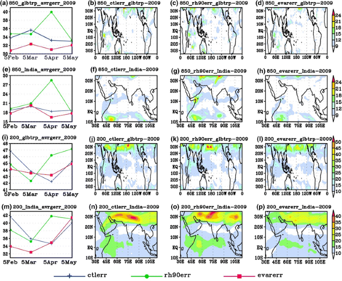
Same as Fig. 10 but for the deficient year 2009
-
3.
Both the upper tropospheric and lower tropospheric wind biases are appeared to be minimum in evarerr during the normal monsoon year of 2003 as revealed from Fig. 10f–h and n–p, respectively over India and adjoining oceanic region. The 850 hPa spatial plot shown in Fig. 10f–h clearly exhibit that the systematic error has been reduced in southern hemisphere, region of cross equatorial flow and low level jets at AS region in evererr. The seasonally mean winds in these regions play crucial roles in determining the seasonal ISMR. Now it may be easily understandable that the weakening of the eastward WVF over the eastern AS (box d) in Fig. 8iv is attributed mainly due to the erroneous low level wind over AS region in the control experiment shown in Fig. 10f. However, the modification of CRH in rhvar improves the wind structure that eventually strengthens the eastward WVF in attributing to the better seasonal ISMR during the year 2003 compared to other sensitivity experiments.
-
4.
Like the normal monsoon year, the year 2009 also shows the minimum error for most of the initial conditions at lower and upper troposphere in rhvar experiment averaged over global tropics and ISM region (Fig. 11a, e, i, m). The April initial condition depicts the minimum wind biases for rhctl and rhvar CRH studies seen in Fig. 11a, e, i. However, the dip in wind bias is observed at March and April initial condition in evarerr and ctlerr, respectively in 200 hPa wind biases averaged over India (Fig. 11m). As such no robust relationship between the initial conditions and the three CRH sensitivity experiments has been observed in the perspective of minimum wind biases.
-
5.
As far as Indian and associated oceanic areas are concerned, the 850 hPa wind biases are also reduced maximum in evarerr during the deficient monsoon shown in Fig. 11f–h as noted for the year 2003. This implies that the proper modulation of the lower tropospheric winds including the cross equatorial flow and the low level jets in AS region during deficient monsoon event are manifested through the most weak eastward WVF in eastern AS and dry BoB (Fig. 9vi) (important factors for subdued rainfall activity during weak monsoon) in rhvar experiment.
-
6.
Similarly, the 200 hPa wind biases show minimum value in evererr over the global tropics including the Indian region compared to ctlerr and rh90err obtained from the spatial plots of Fig. 11j–l and n–p. The higher concentration of upper level cloud condensates in rhctl and rh90 compared to rhvar (Fig. 7b) during the year 2009 indicate more convection and upper level heating (also seen as less TT bias in Figs. 5j, k compared to 5l) that increase the strength of the upper level wind. But, in reality, the upper tropospheric wind should be weak due to the less convection and heating at 200 hPa for weak monsoon condition. Hence, the exaggerated wind produces more biases in rhctl (Fig. 11n) and rh90 (Fig. 11o) compared to rhvar (Fig. 11p) sensitivity experiment in CFSv2.

As it has already been discussed in the introduction chapter that the dynamical feedback to CRH modification is not linear in nature, it is essential to evaluate the nonlinear dynamical processes responsible for error growth in wind field for three sensitivity runs. As the error pattern in Indian region is similar for normal and deficient years, the error energy growth rate budget has been evaluated for the normal year 2003 only. Figure 12a, d, g describe the error growth rates for rhctl, rh90 and rhvar CRH modifications. The rhvar shows the minimum error growth rate in the regions of cross equatorial flow, AS and BoB regions as noted in systematic error (comparing Fig. 10f–h). The Fig. 12b, e, h and c, f, i exhibit the nonlinear advection of error flux and the generation of systematic error energy, respectively. In error flux, positive (negative) value is considered as the nonlinear convergence (divergence) of error. The net error convergence is appeared over the north east sector of India (Fig. 12e) which may be the reason for large systematic error found in the same region (Fig. 10g) in rh90 model run. Comparatively less error growth rate in the cross equatorial flow and the AS regions may be responsible for the less generation of systematic error in those regions seen in rhvar than rhctl experiment (Fig. 12c, i). Moreover, the nonlinear generation of error is also appeared in north-east part of India in rh90 (Fig. 12f) as seen in the corresponding flux term.

The first vertical panel a, d, g describes the spatial distribution of error energy growth rate, the second panel b, e, h shows the spatial plots of nonlinear advection represented by error energy flux whereas the third panel c, f, i exhibits the nonlinear generation of error for rhctl, rh90 and rhvar CRH sensitivity study of CFSv2, respectively during 2003. The unit of all terms in error energy growth rate budget is m2 s−3
4.7 Length of the rainy season
Goswami and Xavier (2005) first showed that the duration of rainy season of ISM might be defined objectively in terms of LRS. The LRS plays a dominating role in determining the variability of seasonal ISM. The northward progression of TCZ which is actually controlled by the easterly vertical shear of mean zonal wind between 200 hPa and 850 hPa levels, determines the meridional extent of south Asian monsoon (Jiang et al. 2004; Goswami and Xavier 2005). Goswami and Xavier (2005) computed that the easterly vertical shear should be around −20 m s−1. (averaged over 50°E–90°E, Equator–15°N) for sustainable northward propagation of TCZ over ISM region. This concept has been applied here to explore the reason behind the weak northward migration of WVF over the IL in the control CRH run (Fig. 8i) during the normal monsoon year. The LRS may be defined as the span of days between the objectively defined onset date (OD) and the withdrawal date (WD) of ISM. The OD has been defined as the date on which the easterly shear first attains the critical value (−20 m s−1) and crosses the line of this critical value (initiation of meridional propagation of TCZ) whereas the WD has been fixed on the day when the shear permanently goes above this critical value (cessation of poleward transport of TCZ) in the daily evaluation of easterly shear following Goswami and Xavier (2005). Figure 13 elucidates the easterly vertical shear of mean zonal wind on daily basis during 122 days of JJAS period of 2003 and 2009 for rhctl (shr_ctl), rh90 (shr_rh90) and rhvar (shr_rhvar) CRH sensitivity experiments of CFSv2 model along with the same for MERRA reanalysis wind (shr_merra_anl). Figure 13a, c represent the wind shear with February and March initial conditions, respectively for the model run and MERRA reanalysis wind during the normal monsoon year 2003 whereas Fig. 13b, d describe the same but for the deficient year 2009. The figures reveal that-

The easterly vertical shear of mean zonal wind in each day averaged over the Indian region (50°E–90°E, Equator–15°N) during 122 days for JJAS period has been plotted for three CRH modifications of CFSv2 and the MERRA reanalysis wind. a, c represent the wind shear for February and March initial conditions, respectively during normal monsoon year 2003 whereas (b, d) describe the same but for the deficient year 2009. The unit of shear is m s−1. The blue line with plus mark, the green line with opaque circle and the magenta line with opaque square represent the vertical shear for rhctl (shr_ctl), rh90 (shr_rh90) and rhvar (shr_rhvar) experiments, respectively. The orange line with transparent triangle mark shows the same (shr_merra_anl) but for MERRA reanalysis wind
-
1.
The LRS is appeared to be lowest for shr_ctl and highest in shr_rhvar during 2003 shown in Fig. 13a as the OD is around 18th June (5th June) for shr_ctl (shr_rh90 and shr_rhvar) and the WD is 30th September for shr_ctl and shr_rh90. In shr_rhvar, the shear is below the magnitude of −20 m s−1 at 30th September implying the LRS is still continued beyond the month of September. Similarly, the rainy season also exhibits with maximum duration in shr_rhvar compared to other experiments for March initial condition (Fig. 13c). However, the vertical shear of MERRA wind (shr_merra_anl) shows the near normal LRS with OD (WD) is around 6th June (28th September). The Fig. 13a reveals that the shr_rhvar line is close to shr_merra_anl line and the control experiment (shr_ctl) underestimates the LRS compared to MERRA reanalysis during the normal monsoon year.
-
2.
During the year 2009, the shr_rhvar shows the larger span of rainy season compared to shr_ctl and shr_rh90 as the OD for rhctl and rhvar (rh90) experiments is 8th June (18th June) and the WD is 1st September (12th September) for rhctl (rh90 and rhvar) CRH studies shown in Fig. 13b for February initial condition. But, the March initial condition (Fig. 13d) has distinguishably exhibited the least LRS in the rhvar run among all the sensitivity studies. The shr_merra_anl exhibits least LRS which is close to the span of the rainy season in shr_rhvar during the deficient year shown in Fig. 13d with OD (WD) is 8th June (27th August) for rhvar and 25th June (10th September) for MERRA wind.
It may be underscored from this subsection that the inhibition of northward migration of WVF may be due to the weak poleward propagation of tropical convection shown by the underestimation of LRS in the control CRH experiment of CFSv2 compared to the length of the season obtained from MERRA wind. The rhvar has convincingly shown the realistic variability in LRS (close to the variability in ISM seasonal span computed from MERRA reanalysis) that again support to better simulation of seasonal ISMR during the normal/deficient monsoon year with respect to other CRH experiments.
5 Summary and conclusions
The skillful dynamical forecast of ISM in a seasonal perspective is imperative as India still depends largely on agriculture. So, an efficient forecast of ISMR ensures our food security and economic growth. At the same time, the sensible prediction of ISM is fascinating, intriguing as well as an extremely challenging job for the community of monsoon meteorologists, because the ISM has been treated as a much complex multi-scale processes controlled by the convection, intra-seasonal oscillations and cloud–atmosphere–land–ocean interactions. In this view, the CFSv2 model (second version of NCEP-CFS model) has been undertaken to explore the effects on the seasonal forecasts of ISM due to the variability in cloud formation causing CRH modification in GCM. As the cloud generates through the manifestation of complicated interactions among radiation, moist convection and microphysical processes driven by large scale circulations, the realistic cloud formation by suitable representation of CRH has a large attribution to the ISMR and its variability. The CFSv2 model has been executed here for two different vertical structures of CRH based on the vertical profile of RH during ISM period obtained from observation and reanalysis data along with the existing profile of the model.
The first profile is the existing structure (abbreviated as rhctl) which is constant CRH (85 %) at model generated cloud-bottom, cloud-middle and cloud-top. The second modified structure (rh90) is also constant as per the existing one but with enhanced magnitude (90 %) of CRH at different cloud levels and the third profile (rhvar) contains the variable magnitude with cloud-bottom, cloud-middle and cloud-top of the CRH value 88, 90 and 89 %, respectively following the observed radio-sounding and MERRA reanalysis profiles. The model has been executed for normal (2003) and deficient (2009) monsoon years to evaluate the variability initialized with four initial conditions taken on the 5th day of the months February, March, April and May of each year. The results are shown and explained by seven thermodynamical and dynamical parameters based on the total twelve runs of CFSv2 model for each year.
The rhvar experiment exhibits more realistic variability in rainfall and PWV biases leading to hypothesize better simulation of cloud formation in comparison with the existing (rhctl) and rh90 experiments without affecting much the biases at other global tropical regions during the contrasting seasons. The increased CRH value at all levels of cloud in rh90 does not imply the better seasonal ISMR and PWV compared to rhvar.
The maximum reduction of cold TT bias in rh90 CRH study during the year 2003 does not indicate the normal monsoon over India. In fact, the improvement in TT is necessary but that in TTG is one of the necessary and sufficient conditions for the realistic variability of seasonal ISMR during normal and deficient years. The rhvar shows the most realistic modulation in TTG during contrasting monsoon seasons among the three CRH experiment.
The latitudinal distribution of upper level (between 100 and 500 hPa) cloud condensates shows more modulation and stronger variability over the northern side of equator (mostly over the ISM region) during rhvar experiment compared to rhctl and rh90 sensitivity experiments. The rhvar experiment is able to modulate convection through OLR in the two contrasting year best among the three CRH studies. The most realistic variability in high cloud fraction and the upward long-wave radiation at the top of the atmosphere are revealed in rhvar CRH modification compared to other CRH experiments which support the modulations of upper level cloud condensates and OLR.
The strong (weak) eastward WVF over eastern AS region, the more (less) northward extent of WVF over IL and the wet (dry) BoB during 2003 (2009) favour for realistic variation of seasonal ISMR in rhvar CRH version compared to other CRH modifications of CFSv2.
As far as the systematic error energy is concerned, it shows minimum value in rhvar experiment at lower and upper tropospheric wind field during 2003 and 2009 (averaged over global tropics as well as the Indian region). The improvement in wind bias over Indian region does not degrade the biases at other global tropical regions. The weakening of eastward WVF in the eastern AS during rhctl experiment in normal monsoon year (one of the key factors for dry bias) may be due to the large systematic error, its growth rate and the nonlinear generation of error responsible for error growth observed in the regions of cross equatorial flow and AS at control run. As such no concrete relationship between the initial conditions and the three CRH runs has been established in the perspective of minimum wind biases.
The inadequate northward extent of WVF in the control CRH study during the year 2003 (another factor for dry bias) is basically attributed to the weak poleward migration of tropical convection zone as seen from the smallest LRS among the three CRH experiments. The rhvar version of the model has distinguishably shown the modulation in LRS, parity with the variability of LRS evaluated from MERRA reanalysis wind field that implies the realistic change in seasonal ISMR during the contrasting years compared to the control and rh90 CRH version of CFSv2.
The most indigenous part of this study is that the proper modification in the CRH of GCM can dictate the large scale system like Indian monsoon by modulating the cloud formation realistically. Many aspects are still unraveled. As the CFSv2 model is a coupled model there is a huge scope of oceanic studies in terms of SST, mixed layer depth, heat budget, air–sea interactions, ocean currents, salinity etc. both in regional and tropical perspective during the boreal summer period. The monsoon intra-seasonal oscillations, its characteristics and predictability studies in extended range mode may also be carried out with modified CFSv2. It can be applied in weather as well as in climate research. The higher resolution of CFSv2 model (T382) may provide better simulations of cloud condensate and cloud fractions that may lead additional improvement in the model. This work has made an avenue for further modification of CFSv2 in cloud–radiation interaction, boundary layer parameterization etc. by keeping the CRH profile following rhvar in CFSv2. The proper choice of CRH in GCM has a seminal role for the better representation of monsoon and its variability by modulating cloud formation realistically. The hypothesis tested in the present study can also be useful for other tropical monsoon regions (e.g. East Asian, African and Australian monsoons) and it will further sustain the GCM development work.
This work may be treated as a first step to initiate a process for improvement of CFSv2 model in the sense that this new version of CFSv2 is able to simulate the normal and deficient seasonal ISM at least qualitatively, supported by thermodynamical and dynamical variables. Actual improvement of the model can be possible only with the biases approaching to zero for contrasting monsoon events and for that it requires further model development.
References
Abhilash S, Sahai AK, Borah N, Chattopadhyay R, Joseph S, Sharmila S, De S, Goswami BN, Kumar A (2014) Prediction and monitoring of monsoon intraseasonal oscillations over Indian monsoon region in an ensemble prediction system using CFSv2. Clim Dyn. doi:10.1007/s00382-013-2045-9
Adler RF, Huffman GJ, Chang A, Ferraro R, Xie P, Janowiak J, Rudolf B, Schneider U, Curtis S, Bolvin D, Gruber A, Susskind J, Arkin P, Nelkin E (2003) The version 2 global precipitation climatology project (GPCP) monthly precipitation analysis (1979–present). J Hydrometeorol 4:1147–1167
Stocker TF et al (2001) Physical climate processes and feedbacks. In: Manabe S, Mason P (eds) Climate change 2001: the scientific basis. Contribution of working group I to the third assessment report of the intergovernmental panel on climate change. Cambridge University Press, Cambridge, pp 419–470
Allan RP, Ringer MA, Slingo A (2003) Evaluation of moisture in the Hadley Centre climate model using simulations of HIRS water vapour channel radiances. Q J R Meteorol Soc 129:3371–3389
Arakawa A, Schubert WH (1974) Interaction of a cumulus cloud ensemble with the large-scale environment, Part I. J Atmos Sci 31:674–701
Bates JJ, Jackson DL (2001) Trends in upper-tropospheric humidity. Geophys Res Lett 28:1695–1698
Blankenship CB, Wilheit TT (2001) SSM/T-2 measurements of regional changes in three-dimensional water vapour fields during ENSO events. J Geophys Res 106:5239–5254
Boer GJ (1993) Systematic and random error in an extended-range forecasting experiment. Mon Weather Rev 121:173–188
Bony S et al (2015) Clouds, circulation and climate sensitivity. Nature Geosci. doi:10.1038/NGEO2398
Cess RD et al (1990) Intercomparison and interpretation of climate feedback processes in 19 atmospheric general circulation models. J Geophys Res 95:16601–16615
Chaudhari HS, Shinde MA, Oh JH (2010) Understanding of anomalous Indian summer monsoon rainfall of 2002 and 1994. Quat Int 213:20–32
Chaudhari HS, Pokhrel S, Saha SK, Dhakate A, Yadav RK, Salunke K, Mahapatra S, Sabeerali CT, Rao SA (2013) Model biases in long coupled runs of NCEP CFS in the context of Indian summer monsoon. Int J Climatol 33:1057–1069
Chaudhari HS, Pokhrel S, Saha SK, Dhakate A, Hazra A (2014) Improved depiction of indian summer monsoon in latest high resolution NCEP climate forecast system reanalysis. Int J Climatol. doi:10.1002/joc.4196
Chen J, Carlson BE, Del Genio AD (2002) Evidence for strengthening of the tropical general circulation in the 1990s. Science 295:838–841
Chung ES, Sohn BJ, Ramanathan V (2004) Moistening processes in the upper troposphere by deep convection: a case study over the tropical Indian Ocean. J Meteorol Soc Jpn 82:959–965
Clough SA, Shephard MW, Mlawer EJ, Delamere JS, Iacono MJ, Cady-Pereira K, Boukabara S, Brown PD (2005) Atmospheric radiative transfer modeling: a summary of the AER codes. J Quant Spectrosc Radiat Transfer 91:233–244
De S (2010) Role of nonlinear scale interactions in limiting dynamical prediction of lower tropospheric boreal summer intraseasonal oscillations. J Geophys Res 115(D21127):1–18. doi:10.1029/2010JD013955
Dessler AE, Sherwood SC (2000) Simulations of tropical upper tropospheric humidity. J Geophys Res 105:20155–20163
Ek M, Mitchell KE, Lin Y, Rogers E, Grunmann P, Koren V, Gayno G, Tarpley JD (2003) Implementation of Noahland-surface model advances in the NCEP operational mesoscale Eta model. J Geophys Res 108:8851. doi:10.1029/2002JD003296
Gadgil S (2003) The Indian monsoon and its variability. Annu Rev Earth Planet Sci 31:429–467
Gadgil S, Rajeevan M, Nanjundiah R (2005) Monsoon prediction—Why yet another failure? Curr Sci 88:1389–1400
Gettelman A, Holton J, Douglass AR (2000) Simulations of water vapor in the lower stratosphere and upper troposphere. J Geophys Res 105:9003–9023
Goswami BN, Xavier PK (2005) ENSO control on the South Asian Monsoon through the length of the rainy season. Geophys Res Lett 32:L18717. doi:10.1029/2005GL023216
Griffies SM, Harrison MJ, Pacanowski RC, Rosati A (2004) A technical guide to MOM4, GFDL Ocean Group Technical Report 5, 337 pp
Hall A, Manabe S (1999) The role of water vapour feedback in unperturbed climate variability and global warming. J Clim 12:2327–2346
Hazra A, Taraphdar S, Halder M, Pokhrel S, Chaudhari HS, Salunke K, Mukhopadhyay P, Rao Suryachandra A (2013a) Indian summer monsoon drought 2009: role of aerosol and cloud microphysics. Atmos Sci Lett 14:181–186. doi:10.1002/asl2.437
Hazra A, Goswami BN, Chen J-P (2013b) Role of interactions between aerosol radiative effect, dynamics and cloud microphysics on transitions of monsoon intraseasonal oscillations. J Atmos Sci 70:2073–2087. doi:10.1175/JAS-D-12-0179.1
Hong S-Y, Pan H-L (1998) Convective trigger function for a mass-flux cumulus parameterization scheme. Mon Weather Rev 126:2599–2620
Iacono MJ, Mlawer EJ, Clough SA, Morcrette JJ (2000) Impact of an improved longwave radiation model, RRTM, on the energy budget and thermodynamic properties of the NCAR Community Climate Model, CCM3. J Geophys Res 105:14873–14890
Jiang X, Li T, Wang B (2004) Structures and mechanisms of the northward propagating boreal summer intraseasonal oscillation. J Clim 17:1022–1039
Kim YJ, Arakawa A (1995) Improvement of orographic gravity wave parameterization using a meso-scale gravity wave model. J Atmos Sci 52:1875–1902
Konwar M, Parekh A, Goswami BN (2012) Dynamics of east-west asymmetry of Indian summer monsoonrainfall trends in recent decades. Gephys Res Lett 39:L10708. doi:10.1029/2012GL052018
Krishnamurti TN, Bedi HS, Subramaniam M (1989) The summer monsoon of 1987. J Clim 2:321–340
Krishnamurti TN, Xue J, Bedi HS, Ingles K, Oosterhof D (1991) Physical initialization for numerical weather prediction over the tropics. Tellus 43AB:53–81
Kumar S, Hazra A, Goswami BN (2014) Role of interaction between dynamics, thermodynamics and cloud microphysics on summer monsoon precipitating clouds over the Myanmar coast and the western ghats. Clim Dyn 43:911–924
Li C, Yanai M (1996) The onset and interannual variability of the Asian summer monsoon in relation to land-sea thermal contrast. J Clim 9:358–375
Lindzen RS, Chou M-D, Hou AY (2001) Does the earth have an adaptive infrared iris? Bull Am Meteorol Soc 82:417–432
Lott F, Miller MJ (1997) A new subgrid-scale orographic drag parametrization: its formulation and testing. Q J R Meteor Soc 123:101–127
Meleshko VP, Wetherald RT (1981) The effect of a geographical cloud distribution on climate: a numerical experiment with an atmospheric general circulation model. J Geophys Res 86:11995–12014
Molod A (2012) Constraints on GCM total water PDF parameters from AIRS and high-resolution models. AMWG2012. www.cesm.ucar.edu/working_groups/Atmosphere
Moorthi S, Pan HL, Caplan P (2001) Changes to the 2001 NCEP operational MRF/AVN global analysis/forecast system. NWS Technical Procedures Bulletin 484:14. http://www.nws.noaa.gov/om/tpb/484.htm
Moorthi S, Sun R, Xiao H, Mechoso RC (2010) Southeast Pacific low-cloud simulation in the NCEP GFS: role of vertical mixing and shallow convection. NCEP Office Note 463, 28 pp. http://www.emc.ncep.noaa.gov/officenotes/FullTOC.html#2000
Murakami T, Nakazawa T, He J (1984) On the 40–50 day oscillations during the 1979 northern hemisphere summer: partII: heat and moisture budget. J Meteorol Soc Jpn 62:469–484
Neena JM, Suhas E, Goswami BN (2011) Leading role of internal dynamics in the 2009 Indian summer monsoon drought. J Geophys Res 116(D13103):1–14. doi:10.1029/2010JD015328
Niranjan Kumar K, Rajeevan M, Pai DS, Srivastava AK, Preethi B (2013) On the observed variability of monsoon droughts over India. Weather Clim Extrem 1:42–50
Pan HL, Wu WS (1995) Implementing a mass flux convective parameterization package for the NMC medium-range forecast model. NMC Office Note 409, 40 pp
Pattnaik S, Abhilash S, De S, Sahai AK, Phani R, Goswami BN (2013) Influence of convective parameterization on the systematic errors of Climate Forecast System (CFS) model over the Indian monsoon region from an extended range forecast perspective. Clim Dyn 41:341–365. doi:10.1007/s00382-013-1662-7
Peters ME, Bretherton CS (2005) A simplified model of the Walker circulation with an interactive ocean mixed layer and cloud-radiative feedbacks. J Clim 18:4216–4234
Pierrehumbert RT (1999) Subtropical water vapour as a mediator of rapid global climate change. In: Mechanisms of global climate change at millennial timescales. Geophysical monograph vol 112. American Geophysical Union, Washington, pp 339–361
Pisharoty PR (1965) Evaporation from the Arabian Sea or the Indian southwest monsoon. In: Results of international Indian Ocean expedition, pp 43–54
Pokhrel S, Rahaman H, Parekh A, Saha SK, Dhakate A, Chaudhari HS, Gairola RM (2012) Evaporation-precipitation variability over Indian Ocean and its assessment in NCEP Climate Forecast System (CFSv2). Clim Dyn 39:2585–2608
Quass J (2012) Evaluating the “critical relative humidity” as a measure of subgrid-scale variability of humidity in general circulation model cloud cover parameterizations using satellite data. J Geophys Res 117:D09208. doi:10.1029/2012JD017495
Rajeevan M, Rohini P, Niranjan Kumar K, Srinivasan J, Unnikrishnan CK (2013) A study of vertical cloud structure of the Indian summer monsoon using CloudSat data. Clim Dyn 40:637–650. doi:10.1007/s00382-012-1374-4
Ramanathan V (1987) The role of earth radiation budget studies in climate and general circulation research. J Geophys Res 92(D4):4075–4095. doi:10.1029/JD092iD04p04075
Rienecker MM et al (2011) MERRA: NASA’s modern-era retrospective analysis for research and applications. J Clim 24:3624–3648. doi:10.1175/JCLI-D-11-00015.1
Rogers RR, Yau MK (1984) A short course in cloud physics, 3rd edn. (International Series in Natural Philosophy), ISBN-10: 0750632151
Saha KR, Bavadekar SN (1973) Water vapor budget and precipitation over the Arabian Sea during the northern summer. Q J R Meteorol Soc 99:273–278
Saha S, Moorthi S, Pan H-L, Wu X, Wang J, Nadiga S, Tripp P, Kistler R, Woollen J, Behringer D, Liu H, Stokes D, Grumbine R, Gayno G, Wang J, Hou YT, Chuang HY, Juang H-MH, Sela J, Iredell M, Treadon R, Kleist D, Delst PV, Keyser D, Derber J, Ek M, Meng J, Wei H, Yang R, Lord S, Dool HVD, Kumar A, Wang W, Long C, Chelliah M, Xue Y, Huang B, Schemm JK, Ebisuzaki W, Lin R, Xie P, Chen M, Zhou S, Higgins W, Zou CZ, Liu Q, Chen Y, Han Y, Cucurull L, Reynolds RW, Rutledge G, Goldberg M (2010) The NCEP climate forecast system reanalysis. Bull Am Meteorol Soc 91:1015–1057
Saha S, Moorthi S, Wu X, Wang J, Nadiga S, Tripp P, Behringer D, Hou Y-T, Chuang H-Y, Iredell M, Ek M, Meng J, Yang R, Mendez MP, van den Dool H, Zhang Q, Wang W, Chen M, Becker E (2013a) The NCEP Climate Forecast System Version 2. J Clim. doi:10.1175/JCLI-D-12-00823.1
Saha SK, Pokhrel S, Chaudhari HS (2013b) Influence of Eurasian snow on Indian summer monsoon in NCEP CFSv2 free run. Clim Dyn 41:1801–1815
Saha SK, Pokhrel S, Chaudhari HS, Dhakate A, Shewale S, SabeerAli CT, Salunke K, Hazra A, Mahapatra S, Rao AS (2014) Improved simulation of Indian summer monsoon in latest NCEP climate forecast system (CFSv2) free run. Int J Climatol 34:1628–1641
Sahai AK, Sharmila S, Abhilash S, Chattopadhyay R, Borah N, Krishna RPM, Joseph S, Roxy M, De S, Pattnaik S, Pillai PA (2013) Simulation and extended range prediction of monsoon intraseasonal oscillations in NCEP CFS/GFS version 2 framework. Curr Sci 104:1394–1408
Shin DW, Cocke S, Larow TE (2003) Ensemble configurations for typhoon precipitation forecasts. J Meteorol Soc Jpn 81:679–696
Shukla J, Sud YC (1981) Effect of cloud-radiation feedback on the climate of a general circulation model. J Atmos Sci 38:2337–2353
Simmons AJ (1982) The forcing of stationary wave motion by tropical diabatic heating. Q J R Meteorol Soc 108:503–534. doi:10.1002/qj.49710845703
Slingo A, Wilderspin RC, Brentnall SJ (1987) Simulation of the diurnal cycle of outgoing longwave radiation with an atmospheric GCM. Mon Weather Rev 115:1451–1457
Sohn B-J, Schmetz J (2004) Water vapor-induced OLR variations associated with high cloud changes over the tropics: a study from Meteosat-5 observations. J Clim 17:1987–1996
Somerville RCJ, Iacobellis SF (1999) Single-Column models, ARM observations, and GCM cloud radiation schemes. Phys Chem Earth B 24:733–740
Sun R, Moorthi S, Mechoso CR (2010) Simulation of low clouds in the Southeast Pacific by the NCEP GFS: sensitivity to vertical mixing. Atmos Chem Phys 10:12261–12272
Sundqvist H, Berge E, Kristjansson JE (1989) Condensation and cloud studies with mesoscale numerical weather prediction model. Mon Weather Rev 117:1641–1757
Tao W-K, Simpson J, Lang S, McCumber M, Adler R, Penc R (1990) An algorithm to estimate the heat budget from vertical hydrometeor profile. J Appl Meteorol 29:1232–1244
Tiedtke M (1993) Representations of clouds in large scale models. Mon Weather Rev 121(3040):3061
Tiedtke M (1996) An extension of cloud-radiation parameterization in the ECMWF model: the representation of subgrid-scale variations of optical depth. Mon Weather Rev 124:745–750
Treadon RE (1996) Physical initialization in the NMC global data assimilation system. Meteorol Atmos Phys 60:57–86
Walcek CJ, Stockwell WR, Chang JS (1990) Theoretical estimates of the dynamic, radiative, and chemical effects of clouds on tropospheric trace gases. Atmos Res 25:53–69
Wang J, Cole HL, Carlson DJ (2001) Water vapor variability in the tropical western Pacific from 20-year radiosonde data. Adv Atmos Sci 18:752–766
Wang Z, Chang CP, Wang B, Jin FF (2005) Teleconnections from Tropics to northern extratropics through a southerly conveyor. J Atmos Sci 62:4057–4070
Webster PJ, Magana VO, Palmer TN, Shukla J, Tomas RT, Yanai M, Yasunari T (1998) Monsoons: processes, predictability and the prospects of prediction. J Geophys Res 103:14451–14510
Wen M, Yang S, Vintzileos A, Higgins W, Zhang R (2012) Impacts of model resolutions and initial conditions on predictions of the Asian summer monsoon by the NCEP climate forecast system. Weather Forecast 27:629–646
Williamson DL, Keihl JT, Ramanathan V, Dickinson RE, Hack JJ (1987) Description of the NCAR community climate model (CCM). NCAR tech note NCAR/TN-285+STR, National Center for Atmospheric Research, Boulder, CO, 112 pp
Wu X, Moorthi KS, Okomoto K, Pan HL (2005) Sea ice impacts on GFS forecasts at high latitudes. In: Eighth conference on polar meteorology and oceanography. American Meteor Society, San Diego 7.4
Xavier PK, Marzin C, Goswami BN (2007) An objective definition of the Indian summer monsoonseason and a new perspective on the ENSO–monsoon relationship. Q J R Meteorol Soc 133:749–764
Xu KM, Randall DA (1996) A semi-empirical cloudiness parameterization for use in climate models. J Atmos Sci 53:3084–3102
Yanai M, Li C, Song Z (1992) Seasonal heating of the Tibetan Plateau and its effects on the evolution of the Asian summer monsoon. J Meteorol Soc Jpn 70:319–351
Zhao QY, Carr FH (1997) A prognostic cloud scheme for operational NWP models. Mon Weather Rev 125:1931–1953
Zhu Y, Newell RE, Read WG (2000) Factors controlling upper-troposphere water vapour. J Clim 13:836–848
Acknowledgments
Authors are thankful to Director; IITM, Dr. A. K. Sahai and Dr. A. Suryachandra Rao, chief program scientists, SERP Group, for providing constant encouragement to carry out the research work. High Power Computing System (HPCS), Prithvi facility is highly acknowledged. Thanks are due to NCEP CFSR, GPCP, MERRA, International Satellite Cloud Climatology Project (ISCCP) and Clouds and Earth’s Radiation Energy Systems (CERES), NASA for the free data availability and University of Wyoming for making available the atmospheric radio sounding data. Authors are also indebted to Mr. K. K. Dani and Mrs. Asha Nath, radiosonding group, IITM for making available some radio-sonding data over Pune. Authors acknowledge highly to Dr. Yu-Tai Hou and Dr. S. Moorthi, NCEP for the helpful discussions. Authors are also thankful to Ferret and Brian Doty, COLA for the use of GrADS software. Anonymous reviewers’ comments are also gratefully acknowledged.
Author information
Authors and Affiliations
Corresponding author
Rights and permissions
About this article

Cite this article
De, S., Hazra, A. & Chaudhari, H.S. Does the modification in “critical relative humidity” of NCEP CFSv2 dictate Indian mean summer monsoon forecast? Evaluation through thermodynamical and dynamical aspects. Clim Dyn 46, 1197–1222 (2016). https://doi.org/10.1007/s00382-015-2640-z
Received:
Accepted:
Published:
Issue Date:
DOI: https://doi.org/10.1007/s00382-015-2640-z