
Abstract
The slope measured by a wavefront sensor has good sparsity in the frequency domain, so the application of compressed sensing technology to wavefront detection can significantly improve the measurement speed of the wavefront signal. In this study, the sparsity adaptive matching pursuit algorithm (SAMP) was used to reconstruct the distorted wavefront. The numerical analysis results show that, compared with the compressed sampling matching pursuit algorithm (CoSAMP) and the orthogonal matching pursuit algorithm (OMP), the reconstruction time of the SAMP algorithm is short and it has a high reconstruction accuracy. An adaptive optics system experiment was built to verify the ability of the SAMP algorithm to correct the beam wavefront distortion. The results show that after the distorted wavefront was reconstructed by the SAMP, CoSAMP, and OMP algorithms, the peak to valley values of the wavefront were reduced from 2.67 µm before correction to 0.03 µm, 0.038 µm and 0.05 µm after correction. The effectiveness of the SAMP algorithm in reconstructing a distorted wavefront was verified.
1 Introduction
In wireless optical communication systems, the laser beam can experience interference due to atmospheric turbulence during transmission [1]. This produces random fluctuations in phase, resulting in diffusion, drift, jitter, and other changes in the received beam, thus reducing the quality of the communication system. The application of adaptive optics (AO) in a wireless optical communication system can effectively compensate for the wavefront distortion caused by atmospheric turbulence, actively adapt to changes in the external environment, overcome dynamic interference, and thereby improve the quality of the system [2, 3]. The AO system detects the beam through a wavefront sensor and reconstructs the wavefront phase information of the beam, and then corrects it using a deformable mirror. In the traditional reconstruction method, a Shack–Hartmann wavefront sensor (SH-WFS) is used to measure the average slope gx and gy of the wavefront distortion along the x- and y-axes, respectively, and the wavefront phase value is calculated from the average slope of each sub-aperture [4, 5]. This method requires the measurement of a large amount of slope data. Therefore, the calculation is quite difficult, and the processing speed is slow.
To remedy these shortcomings, compressed sensing (CS) technology can be used to measure the slope of the wavefront distortion from sparse sampling. A nonlinear reconstruction algorithm can then be used for reconstruction of the slope, and the phase distribution is then obtained. Results have shown that this method can significantly reduce data redundancy and the loads of data transmission, storage, and processing. In 2006, Donoho proposed the compressed sensing theory, which was found to overcome the defects of the Nyquist sampling theorem and successfully realize signal sampling and compression [6,7,8]. In 2012, Rostami proposed the use of a sparse representation to measure the compressed wavefront [9]. A numerical simulation method was adopted to verify the feasibility of the compressed sensing theory for the measurement of the wavefront. In 2016, Chow proposed a compression wavefront sensing method based on a sparse Zernike representation to reconstruct the slope in the Zernike domain [10]. The reconstruction results shown that the compressive sensing reconstruction had a lower reconstruction error compared with the pattern reconstruction. With the development and application of compressed sensing technology, many reconstruction algorithms have been developed, such as the combinatorial optimization algorithm, convex optimization algorithm, and greedy pursuit algorithm. The combination optimization algorithm requires sampling observation under specific conditions, so the reconstruction efficiency is high, but the reconstruction accuracy needs to be improved. The convex optimization algorithm has a high reconstruction accuracy, but it is computationally complex and inefficient. The greedy pursuit algorithm considers both running efficiency and sampling efficiency, and is favored because of its simple algorithm structure and small computational requirements. Major algorithms in this category include Stagewise orthogonal matching pursuit algorithm (StOMP) [11], subspace pursuit algorithm (SP) [12], orthogonal matching pursuit algorithm (OMP) [13], and compressed sampling matching pursuit algorithm (CoSAMP) [14]. However, all of these algorithms require the signal sparseness to be prior information. In practical applications, the sparsity of the signal is often unknown or variable.
In response to the above problems, this study used the sparsity adaptive matching pursuit algorithm (SAMP) [15] to reconstruct the wavefront slope signal, which solves the problem of unpredictable sparsity. This algorithm combines the staged idea of the StOMP algorithm and the back-screening idea of the SP algorithm. The true sparsity of the signal is gradually approximated through iterations, which greatly increases the scope of application of the algorithm. This study analyzed the applicability of the SAMP algorithm under the conditions of weak turbulence, medium turbulence, and strong turbulence and its performance under different compression ratios, and compared the reconstruction performance of the algorithm with the CoSAMP algorithm and the OMP algorithm.
2 Theoretical research
2.1 Principle of the adaptive optics system
The working principle of an adaptive optics system is illustrated in Fig. 1. The system consists of a wavefront sensor, wavefront controller, and wavefront corrector. When the signal light propagates through the atmosphere, a distorted wavefront is produced due to turbulence. The system measures the wavefront distortion of the received beam in real time using the wavefront sensor and feeds the measurements back to the wavefront controller to reconstruct the distorted wavefront, providing a real-time control signal for the wavefront corrector.

Schematic diagram of adaptive optics system
2.2 Working principle of Shack–Hartmann wavefront sensor
The SH-WFS is a commonly used sensor for measuring wavefront slopes. It is composed of a microlens array and high-speed charge-coupled device (CCD) image sensor [16], as shown in Fig. 2. When a plane wave is incident on the microlens array, the CCD is used to collect the image at the focal plane of the array, and the reference image points are located in the center of each unit of the array. In contrast, when the distorted wavefront is incident on the microlens array, depending on the degree of distortion, the positions of the image points collected at the focal plane will be different from the reference image points.

Schematic diagram of Shack–Hartmann wavefront sensor
The offset of each image point is proportional to the wavefront slope in the x- and y-directions of the corresponding sub-aperture, and the corresponding relationship is shown in Eq. (1)
where gx and gy are the wavefront slopes in the x- and y-directions, respectively, f is the distance from the microlens to the focal point, λ is the wavelength of the light wave, and ΔCx and ΔCy are the offsets in the x- and y-directions, respectively. The average slope of the wavefront in each sub-aperture is calculated by measuring the offset of the light spot in the x- and y-directions, and the phase distribution of the entire distorted wavefront can be obtained using the reconstruction algorithm.
2.3 Compressed sensing technique and SAMP algorithm
-
1.
Compressed sensing technique
The compressed sensing technique consists of a sparse representation of the signal, design of the observation matrix, and reconstruction. Figure 3 shows a block diagram of compressed sensing.
Fig. 3 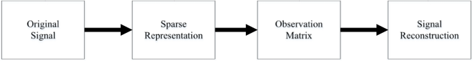
Block diagram of compressed sensing technique
Let gxRN×1 and gyRN×1 be slope signals that need sparse representation in the x- and y-directions, respectively. Their sparse forms can be expressed as
$$g_{x} = \psi \theta_{x} ,g_{y} = \psi \theta_{y} ,$$(2)where ΨRM×N is the sparse matrix, and Ψ is an orthonormal basis, θxRN×1 and θyRN×1 are the sparse representation coefficients.
The observation matrix \(\Phi \in {R}^{M\times N}\) (M is the dimension of the observation obtained by the slope signals, M << N) is used for sampling and compressing the sparse signal, where Φ is a Gaussian random matrix [18] satisfying the constraint isometric property (RIP) [17]. By a linear representation of the signal, the measured matrix of the slope signals after sampling compression can be obtained as shown in Eq. (3) [19]
$$f_{x} = \Phi g_{x} ,f_{y} = \Phi g{}_{y}.$$(3)Substituting Eq. (2) into Eq. (3) to yields Eq. (4)
$$f_{x} = \Phi \Psi \theta_{x} = A\theta_{x} ,f_{y} = \Phi \Psi \theta_{y} = A\theta_{y} ,$$(4)where A = ΨRM×N is the sensing matrix. The process of signal reconstruction is based on the measured matrix fx and fy to reconstruct the sparse estimate value \(\widehat{\theta }_{x}\) and \(\widehat{\theta }_{y}\) of the slope signals gx and gy, and the process can be expressed as the 0-norm optimization problem
$$\begin{gathered} \mathop {\min }\limits_{{\theta_{xi} }} \left\| {\theta_{xi} } \right\|_{0} \begin{array}{*{20}c} {} & {} \\ \end{array} {\text{s.t}}{.}\begin{array}{*{20}c} {} & {} \\ \end{array} f_{xi} = A\theta_{xi} \hfill \\ \mathop {\min }\limits_{{\theta_{yi} }} \left\| {\theta_{yi} } \right\|_{0} \begin{array}{*{20}c} {} & {} \\ \end{array} {\text{s.t}}{.}\begin{array}{*{20}c} {} & {} \\ \end{array} f_{yi} = A\theta_{yi} . \hfill \\ \end{gathered}$$(5)Compressed sensing theory states that when the signal itself or in a certain transform domain is sparse, the original signal can be reconstructed with high precision from a small amount of sampled data using the reconstruction algorithm. In the adaptive optics system, the slope signals collected by the wavefront sensor meet the requirements of sparsity and irrelevance. Therefore, it is feasible to apply the compressed sensing theory to distorted wavefront reconstruction, which not only improves the sampling speed of the signal but also reduces information redundancy.
-
2.
SAMP algorithm
The SAMP algorithm does not need to know the sparsity of the signal and adjusts the iteration step by adaptive method to approach the original signal step by step. At the beginning of the iteration, the initial step size is a small value, and the step size is gradually expanded by stages. With the increase of the number of iterations, the step size is increased when the residual value is non-decreasing than that of the last one, and the true sparsity of the signal is gradually approached. The algorithm steps are shown in Table 1.
Table 1 SAMP algorithm flow

2.4 Evaluation indicators
-
1.
Peak signal-to-noise ratio
The peak signal-to-noise ratio (PSNR) represents the ratio of the maximum possible power of a signal to the power of the noise that affects its representation accuracy. This is defined as follows:
$${\text{PSNR}} = 10\log_{10} \left( {\frac{{(2^{n} - 1)^{2} }}{{{\text{RMS}}}}} \right),$$(6)where n is the number of bits of each sampled value.
-
2.
Root-mean-square error
The root-mean-square (RMS) value of the wavefront characterizes the degree of deviation of the wavefront of the measured beam from the ideal wavefront, and is defined as follows:
$$\begin{gathered} {\text{RMS}} = \sqrt {\frac{1}{\pi }\int_{0}^{{2\pi }} {\int_{0}^{1} {\left[ {\Delta \psi \left( {\rho ,\theta } \right) - \overline{{\Delta \left( {\rho ,\theta } \right)}} } \right]^{2} \rho d\rho d\theta } } } \hfill \\ = \sqrt {\overline{{\Delta \psi \left( {\rho ,\theta } \right)^{2} }} - \left( {\overline{{\Delta \psi \left( {\rho ,\theta } \right)}} } \right)^{2} } , \hfill \\ \end{gathered}$$(7)where ψ(ρ, θ) is the wavefront distribution function of the measured beam, and Δψ(ρ, θ) is the deviation between the measured and ideal beams.
-
3.
Peak and valley value of wave front
Peak to valley (PV) represents the numerical difference between the highest and lowest points of the measured beam wavefront, defined as follows:
$$PV = \max \left( {\Delta \psi \left( {\rho ,\theta } \right)} \right) - \min \left( {\Delta \psi \left( {\rho ,\theta } \right)} \right).$$(8)
3 Analysis of simulation results
In this study, the covariance matrix of the Zernike polynomial coefficients [20, 21] expanded by K–L function was used to simulate the original distorted wavefront phase φ(x, y) of the beam after transmission through atmospheric turbulence. Then, based on the principle of compressed sensing, the slope signal of wavefront distortion was sparsely measured, the wavefront slope value was reconstructed, and the atmospheric turbulence distortion wavefront phase φ'(x, y) was restored. The sparse dictionary was selected as the discrete Fourier transform dictionary, the observation matrix Φ was a Gaussian random matrix, the Zernike polynomial was the first 30 orders, the telescope aperture size was D = 20 cm, the grid sample size of phase screen was 128 × 128, the phase screen size was 0.4 m, and r0 is the atmospheric coherent length. For the gentle turbulent condition, D/r0 is around 2. For the moderate turbulent condition, D/r0 is around 10. For the relative strong turbulent condition, /r0 is around 17 [22].
3.1 Analysis of reconstruction effect under different turbulence
When the compression ratio (M/N) was 0.6, Fig. 4 shows the distortion phase diagram of the original wavefront and the SAMP algorithm reconstructed wavefront under the conditions of weak turbulence, medium turbulence, and strong turbulence.

Distortion phase diagrams: a original distorted wavefront; b SAMP algorithm reconstructed wavefront
Figure 4a1–a3 are the original distortion wavefronts generated when D/r0 = 2, D/r0 = 10, and D/r0 = 20, respectively, and Fig. 4b1–b3 are the distorted wavefronts reconstructed by the SAMP algorithm when D/r0 = 2, D/r0 = 10, and D/r0 = 20, respectively. It can be seen that as the intensity of atmospheric turbulence increases, the degree of wavefront distortion increases. The wavefront reconstructed by the SAMP algorithm under all turbulence conditions was close to the original distorted wavefront, indicating that the algorithm has good applicability.
3.2 Analysis of the influence of different compression ratios on reconstruction accuracy
Under the condition of D/r0 = 10, the influence of different compression ratios of the SAMP algorithm on the reconstruction accuracy was analyzed. The results are shown in Fig. 5a–d which shows the wavefront phase diagrams with compression ratios of 0.1, 0.3, 0.5, and 0.7, respectively.

Distorted wavefront diagrams reconstructed by SAMP algorithm: a compression ratio = 0.1; b compression ratio = 0.3; c compression ratio = 0.5; d compression ratio = 0.7
The results in Fig. 5 show that the reconstruction effect improves as the compression ratio increases. Table 2 shows a comparison of the signal-to-noise ratio and reconstruction time of the SAMP algorithm for different compression ratios. It can be clearly seen that as the compression ratio increases, the peak signal-to-noise ratio of the SAMP algorithm increases, and therefore, the reconstruction effect gradually improves, but the reconstruction time also increases.
3.3 Analysis of reconstruction performance of different algorithms
To quantitatively analyze the superiority of the SAMP algorithm, the CoSAMP algorithm and the OMP algorithm were used to reconstruct the distorted wavefront for D/r0 = 10 and a compression ratio of 0.6. The results are shown in Fig. 6, where Fig. 6a, b shows the wavefront phase reconstructed by the CoSAMP and OMP algorithms, respectively. Comparing Fig. 6 with the original distorted wavefront in Fig. 4a2 and the wavefront reconstructed by the SAMP algorithm in Fig. 4b2, it can be seen that the phase of the wavefront reconstructed by the SAMP algorithm is also reconstructed by the OMP and CoSAMP algorithms. The reconstructed wavefront is closer to the original distorted wavefront for all three algorithms.

a CoSAMP algorithm reconstructed wavefront; b OMP algorithm reconstructed wavefront
Figure 7 shows the RMS values of the three algorithms. As seen in the figure, as the number of iterations increases, the RMS value decreases. In the first 10 iterations, the RMS value drops sharply. As the number of iterations increases, the amount of decrease lessens and the curves gradually flatten until they converge, and the value stabilizes. Comparing the three curves, it can be seen that the SAMP algorithm has a faster convergence rate than the CoSAMP and OMP algorithms, and the relative error when using the SAMP algorithm is smaller than that when using the CoSAMP and OMP algorithms.

The root-mean-square error changes with the number of iterations
To further quantitatively analyze the reconstruction performance of the SAMP algorithm, we calculated the peak signal-to-noise ratio of the three algorithms for different numbers of iterations, as shown in Fig. 8. It can be seen that when the number of iterations increases, the peak signal-to-noise ratio of the three algorithms is improved. In the first eight iterations, the PSNR value of the SAMP algorithm is nearly twice as high as that of the CoSAMP algorithm and approximately three times higher than that of the OMP algorithm. After 15 iterations, the increase in the PSNR value gradually flattens. For the same number of iterations, the performance of the SAMP algorithm is significantly better than that of the CoSAMP and OMP algorithms.

The PSNR changes with the number of iterations
Table 3 shows the reconstruction times of the three algorithms when the compression ratio is 0.6. The reconstruction time of the CoSAMP algorithm is twice that of the SAMP algorithm, and the reconstruction time of the OMP algorithm is three times that of the SAMP algorithm. In summary, when the compression ratio is the same, the reconstruction time of the SAMP algorithm is the shortest, and the SAMP algorithm has a better reconstruction efficiency.
4 Experimental research
To verify the correctness of the theoretical results, the research team built an adaptive optical system to correct the distortion wavefront reconstructed by the SAMP, CoSAMP, and OMP algorithms. The experimental setup is shown in Fig. 9. The wavefront sensor is a Shack–Hartmann wavefront sensor HASO4-FIRST, and the deformable mirror is a model DM69 made by ALPAO. The light source was emitted by a laser and passed through a 4F system composed of lenses L1 (f = 30 mm) and L2 (f = 200 mm) to complete the beam expansion and collimation. The light beam was reflected by a beam splitting prism and then incident on the deformable mirror surface. The deformable mirror driver controlled the deformable mirror to produce a certain surface shape to compensate and correct the distorted wavefront. The corrected beam was transmitted through the beam splitter again and was incident on the 4F system composed of L3 (f = 175 mm) and L4 (f = 75 mm) for beam reduction. The wavefront sensor was located at the focal point of the L4 lens to detect the wavefront and transmit the detection information to the wavefront controller (computer). The computer reconstructed the distorted wavefront through compressed sensing technology, obtained the phase, established the relationship between the voltage and the phase, and obtained the control voltage, which was sent to the deformable mirror for wavefront correction, forming a closed-loop correction system of adaptive optics. The atmospheric turbulence in the experimental setup includes two parts, one part is the aberration of optical components and the aberration introduced in the process of optical path setup, and other part is to use the deformable mirror to generate a random phase distortion before PID control algorithm correcting the distorted wavefront. The deformable mirror in the experimental setup is used to generate a random phase distortion and compensate the whole wavefront distortion of the system.

Adaptive optics system: a schematic diagram; b physical diagram
The PID control algorithm [23] was used to correct the wavefront distortion in the closed-loop state, where the algorithm parameter kp = 0.1. Figure 10a–c shows the phase maps of the distorted wavefront reconstructed by the SAMP, CoSAMP, and OMP algorithm after correction, respectively, and the Zernike coefficient value of the wavefront after correction is shown in Fig. 11. It can be seen that the correction result of the distorted wavefront reconstructed by SAMP is better than that of the CoSAMP and OMP algorithms, and the Zernike coefficient value of the distorted wavefront after corrected by PID control algorithm with the wavefront reconstructed by SAMP is smaller than that of the CoSAMP and OMP algorithms.

Different algorithms reconstruct the phase map after distortion wavefront correction: a SAMP algorithm; b CoSAMP algorithm; c OMP algorithm

The Zernike coefficient value of the wavefront after correction
Figure 12 shows the PV value change curve after reconstructing the distorted wavefront by the SAMP, CoSAMP, and OMP algorithms and correcting by the PID control algorithm. As shown in the figure, the PV value curve after correcting the distorted wavefront reconstructed by the SAMP algorithm converges to 0.03 μm at the 65th iteration. For the CoSAMP and OMP algorithms, and the corrected PV curves converged to 0.038 μm at the 131th and 0.05 μm at the 200th times, respectively.

PV values after distorted wavefront correction by PID control algorithm with three algorithms reconstructing the distorted wavefront
5 Conclusion
In this study, compressive sensing technology was used in the reconstruction of the distorted wavefront in adaptive optics to improve the efficiency of wavefront detection. The proposed SAMP method compresses the slope signal and shortens the wavefront sampling requirement to meet the accuracy requirements of the wavefront measurement time. At the same time, the reconstruction effect of the SAMP wavefront reconstruction algorithm under environments of varying turbulence and the influence of different compression ratios on the reconstruction accuracy were analyzed. The results show that the higher the compression ratio, the better the reconstruction accuracy. The reconstruction performance of the SAMP algorithm was compared with that of the CoSAMP and OMP algorithms. The root-mean-square error, peak signal-to-noise ratio, and reconstruction time of the three algorithms were compared, and the PV values of the three algorithms reconstructed after the distortion wavefront correction were analyzed through correction experiments. The results showed that the SAMP algorithm had a higher reconstruction accuracy and faster convergence speed than the CoSAMP and OMP algorithms.
References
V.A. Banakh, A.V. Falits, Turbulent broadening of Laguerre-Gaussian beam in the atmosphere[J]. Opt. Spectrosc. 117(6), 942–948 (2014)
R.K. Tyson, Principles of adaptive optics, Fourth Edition[M] (CRC Press, Boca Raton, 2015)
S.R. Restaino, J.R. Andrews, T. Martinez et al., Adaptive optics using MEMS and liquid crystal devices[J]. J. Opt. A Pure Appl. Opt. 10(6), 064006 (2008)
D.R. Neal, J. Copland, D.A. Neal, Shack-Hartmann wavefront sensor precision and accuracy[C]. Adv. Char. Tech. Opt. Semicond. Data Storage Compon. 4779, 148–160 (2002)
J. Primot, Theoretical description of Shack–Hartmann wave-front sensor[J]. Opt. Commun. 222(1), 81–92 (2003)
E.J. Candes, J. Romberg, T. Tao, Robust uncertainty principles: exact signal reconstruction from highly incomplete frequency information[J]. IEEE Trans. Inf. Theory 52(2), 489–509 (2006)
D.L. Donoho, Compressed sensing[J]. IEEE Trans. Inf. Theory 52(4), 1289–1306 (2006)
E.J. Candes, T. Tao, Near-optimal signal recovery from random projections: universal encoding strategies[J]. IEEE Trans. Inf. Theory 52(12), 5406–5425 (2006)
M. Rostami, Image deblurring using derivative compressed sensing for optical imaging application[J]. IEEE Trans. Image Process. 21(7), 3139–3149 (2012)
E.C.M. Tik, X. Wang, N.Q. Guo, et al. Investigation on compressed wavefront sensing in freeform surface measurements[C]. In: 4th International Conference on Photonics, Optics and Laser Technology, pp. 154–159 (2017)
D.L. Donoho, Y. Tsaig, I. Drori et al., Sparse solution of underdetermined systems of linear equations by stagewise orthogonal matching pursuit[J]. IEEE Trans. Inf. Theory 58(2), 1094–1121 (2012)
W. Dai, O. Milenkovic, Subspace pursuit for compressive sensing signal reconstruction[J]. IEEE Trans. Inf. Theory 55(5), 2230–2249 (2009)
S.K. Sahoo, A. Makur, Signal recovery from random measurements via extended orthogonal matching pursuit[J]. IEEE Trans. Signal Process. 63(10), 2572–2581 (2015)
D. Needell, J.A. Tropp, CoSaMP: iterative signal recovery from incomplete and inaccurate samples[J]. Appl. Comput. Harmon. Anal. 26(3), 301–321 (2009)
T.T. Do, L. Gan, N. Nguyen, et al. Sparsity adaptive matching pursuit algorithm for practical compressed sensing[C]. In: 2008 42nd Asilomar Conference on Signals, Systems and Computers, pp. 581–587 (2008)
M. Rais, J.M. Morel, C. Thiebaut et al., Improving wavefront sensing with a Shack–Hartmann device[J]. Appl. Opt. 55(28), 7836–7846 (2016)
E.J. Candes, The restricted isometry property and its implications for compressed sensing[J]. C.R. Math. 346(9–10), 589–592 (2008)
R. Baraniuk, M. Davenport, R. Devore et al., A simple proof of the restricted isometry property for random matrices[J]. Constr. Approx. 28(3), 253–263 (2008)
H. Rauhut, K. Schnass, P. Vandergheynst, Compressed sensing and redundant dictionaries [J]. IEEE Trans. Inf. Theory 54(5), 2210–2219 (2008)
R.J. Noll, Zernike polynomials and atmospheric turbulence[J]. J. Opt. Soc. Am. 66(3), 207–211 (1976)
N.A. Roddier, Atmospheric wavefront simulation using Zernike polynomials[J]. Opt. Eng. 29(10), 1174–1180 (1990)
C. Liu, S.Q. Chen, X.Y. Li et al., Performance evaluation of adaptive optics for atmospheric coherent laser communications. Opt. Express 22(13), 15554–15563 (2014)
Z.Y. Zheng, C.W. Li, B.M. Li et al., Analysis and demonstration of PID algorithm based on arranging the transient process for adaptive optics[J]. Chin. Opt. Lett. 11(11), 110101 (2013)
Funding
The Key Industrial Innovation Chain Project of Shaanxi Province (Grant number 2017ZDCXL-GY-06-01, 2020ZDLGY05-02); the Xi’an Science and Technology Planning Project (Grant number 2020KJRC0083); Scientific Research Plan Projects of Shaanxi Education Department (18JK0341).
Author information
Authors and Affiliations
Corresponding author
Ethics declarations
Conflict of interest
The authors declare that there are no conflicts of interest.
Additional information
Publisher's Note
Springer Nature remains neutral with regard to jurisdictional claims in published maps and institutional affiliations.
Rights and permissions
About this article

Cite this article
Ke, X., Wu, J. & Hao, J. Distorted wavefront reconstruction based on compressed sensing. Appl. Phys. B 128, 107 (2022). https://doi.org/10.1007/s00340-022-07827-6
Received:
Accepted:
Published:
DOI: https://doi.org/10.1007/s00340-022-07827-6