
Abstract
In this paper, a modified spectral holography structure is demonstrated. Combining the direct space-to-time pulse shaping theory with the modified structure, we can convert a spatial domain x–y image into a y–t image, where one spatial dimension is now transformed into the time domain. Thus we realize the space-to-time or parallel-to-serial conversion. As an example, we generate the temporal equivalent of letter “A”, where each pixel of the image is now represented by a short optical pulse. As a possible application of our scheme, we demonstrate the generation of trains of a femtosecond pulse sequence by our structure. The results of the paper can be applied in ultrashort pulse shaping, ultrafast communication and other relevant areas.
1 Introduction
To fully utilize the bandwidth and efficiency of fiber-optic communication systems, high-rate optical pulse sequences could be beneficial. Generation of trains of femtosecond pulses belongs to the field of pulse shaping. Reviews of various pulse shaping techniques up to 1998 can be found in Refs. [1] and [2]. The most widely used pulse shaping schemes are based on Fourier synthesis and direct space-to-time shaping techniques. In this paper, we propose a scheme to perform space-to-time or parallel-to-serial pulse shaping conversion by the combination of a direct space to time pulse shaping theory with spectral holography structure.
Spectral holography, a technique to store and reconstruct ultrashort pulse by holographic recording of spatially dispersed optical frequency components, was first proposed by Mazurenko in 1990 [3]. With spectral holography, recall, time-reversal, convolution, correlation and matched filtering of the shaped waveform have been realized by Weiner [4–6]. In hybrid spectral holography systems, the spatial and temporal information of the input pulses is mixed, which allows conversion of ultrashort pulse from the spatial domain into time domain and vice versa.
Serial-to-parallel and parallel-to-serial conversion are useful for high-speed communication and information processing. There are lots of papers about the serial-to-parallel conversion. In 1990s, sub-Tbits/s time-to-space mapping was demonstrated by Ema and his coworkers [7], later they performed femtosecond pulse conversion at faster rates [8]. Nuss et al. demonstrated femtosecond pulse mapping in a spectral holography setup by reading it out with continuous-wave diode laser [9]. Sun performed serial-to-parallel data conversion used in long-distance optical communication networks [10]. Later Chung and Weiner reported the first time-to-space converter operating at optical communications wavelength [11]. To improve the conversion efficiency, Kanan and Weiner utilized temperature-tuned noncritical phase matching in KNbO3 nonlinear crystal to reach 50% conversion efficiency [12]. Efficiency can be further increased by collinear nondegenerate phase-matched sum-frequency [13]. Other time-to-space conversion methods via three-wave mixing and four-wave mixing are also demonstrated [14–18].
Parallel-to-serial conversion techniques are useful for the realization of ultrahigh bit-rate optical communication because they form easily parallel-to-serial transmitters and serial-to-parallel receivers. Spectral holography and spectral nonlinear optics can also be utilized for the space-to-time conversion, or parallel-to-serial conversion [19–30]. Mazurenko was the first scientist to theoretically discuss the space-to-time conversion [3, 19]. Later, by taking advantage of the time–space dualities that exist in Fourier-transform optical systems, Nuss experimentally demonstrated the conversion of a spatial image into temporal image [20]. Based on the nonlinearities in the recording process, Ding’s group demonstrated edge enhancement in space-to-time conversion [21]. The spectral holography based space-to-time conversion was also pursued by Fainman’s group [10, 22–24]. In his group, Sun demonstrated parallel-to-serial data conversion, which can be used in long-distance optical communication networks [10]; To realize all-optical communication, Marom relied on real-time holographic materials for conversion of information between spatial and temporal domain [22]; By four wave mixing, Marom realized femtosecond rate space-to-time conversion [24]. McKinney and coworkers presented a novel direct space-to-time pulse shaper operating in the 1.5 μm optical communications band, which enables generation of continuous optical pulse sequences at a rate of 100 GHz [25].
In this paper, we propose a modified spectral holography structure to realize the conversion of spatial image into temporal information. Functionally, the spectral holography structure acts as an optical parallel-to-serial converter. Moreover we systematically study on the recording and readout of spectral holography by two ultrashort pulses with both the spatial and temporal information. We also show how this structure can realize the conversion of a spatial image into its time-encoded temporal image.
2 Spectral decomposition of a single pulse
For better understanding of the space–time properties of wave fields, we first discuss the spectral decomposition of a single pulse, then discuss the recording and readout of spectral holography.
Figure 1 is the diagram of the optical spectral instrument, which is similar to that of the spatial holography, different in that there has a grating G. G is placed in the front focal plane of lens L, and performs the angular spectral decomposition of the incident pulse along x. The spectrum plane S coincides with the back focal plane of the lens L. x is the transverse coordinate in the plane of the grating. For simplicity, the scales of both the front and back focal planes of the lens L are equal.

Spatial spectral decomposition of a single pulse
Supposing that an ultrashort pulse with both the spatial and temporal modulations incidents on the spectral instrument,
where a(x,y) represents the spatial distribution, with y axis perpendicular to the direction of the spectral decomposition x axis; r(t) is temporal envelope. ω 0 is the carrier frequency, and c.c represents complex conjugate.
The grating diffracts the incident pulse according to the temporal frequencies it included, so we need to introduce the spectrum R(ω) of the temporal envelope,

where ω is the frequency shifting from the central frequency ω 0.
In Fourier optics, we are interested in the amplitude description of the spectral instrument action. One can describe the angular spectral decomposition of pulse by grating as a result of the passage of plane waves through a transparency which has the following complex amplitude transmission [31]:

where \(\beta = 2\pi cm/[\omega_{0}^{2}d\cos(\gamma_{0})]\) is the dispersion of the diffraction grating. c is the velocity of light in free space; k=ω 0/c is the wavenumber, m is the diffraction order (here we use m=1); d is grating period and γ 0 is the diffraction angle of the central frequency component of the pulse.
Just after the grating G, the field distribution for each component of the incident pulse becomes,
Here the astigmatism α=cos(θ)/cos(γ 0), with θ is the incident angle of the pulse. As the incident angle and diffraction angle of central wavelength component are defined, α is determined.
According to Fourier optics, the field on the back focal plane of the lens L is the Fourier transform of the field on the front focal plane, the Fourier transform of (4) is
In our treatment, we omit the constant coefficients. f x and f y represent spatial frequency variables corresponding to spatial variables x and y. A (f x ,f y ) represents Fourier transform of a(x,y).
3 Recording of spectral holography with a filter
To record a spectral holography, two coherent pulses must be incident on the spectral instrument of Fig. 1. The expressions of the two pulses are

where a i (x,y) and r i (t) (i=1,2) represent the spatial distributions and temporal envelopes of the two pulses respectively. Assuming the two recording pulses have the same central frequency ω 0.
From the discussion of Sect. 2, we can get the field distributions of these two incident pulses on the spectral plane S,


where \(f_{x} = \frac{x}{\lambda f}\). f is focal length of lens L and λ is the wavelength of the incident pulse component. \(A_{1}(\frac{f_{x}}{\alpha},f_{y})\) and \(A_{2}(\frac{f_{x}}{\alpha} ,f_{y})\) are Fourier transforms of spatial field distributions a 1(x,y) and a 2(x,y).
According to the property of delta function, in (7a) and (7b), the same frequency components of the two incident pulses locate at different positions on the spectral plane S,


In order to acquire the interference fringe of the two sets spectral distributions, we must ensure the same frequency components in two pulses located at the same position on plane S, that is, x 1=x 2, then we have
From the definition of \(\beta = 2\pi cm/[\omega_{0}^{2}d\cos(\gamma_{0})]\), we know β is determined by the diffraction angle γ 0 of the central frequency component, while γ 0 is determined by incident angle θ. So to acquire the interference fringe, the two incident pulses must have the same incident angle θ, that is, they should incident on the grating in parallel.
At the spectral plane S, if we put a holographic recording media, the interference intensity can be recorded. If before the recording media we put an ideal thin slit, and make the transverse slit locate at x=x 0, the field distributions just after the slit are


Substituting (7a), (7b) and (9) and \(f_{x} = \frac{x}{\lambda f}\) into (10a) and (10b), the filed distributions just after the slit and before the holographic recording media are


For simplicity, assuming \(\frac{\frac{x_{0}}{\lambda f} - k\beta \omega}{ \alpha} = f_{\omega}\), which is a function of frequency, and has nothing to do with axis x. That is, F′( ,) is just a function of frequency.
The interference field on the recording media is
The holographic media records the intensity distribution of the interference field,
Assuming the recording is linear and neglecting effects due to the finite spectral resolution of the pulse shaping apparatus, after developing and fixing, we acquire a holographic plate with transmittance linearly proportional to T(ω,f y ). The transmittance is dependent on the variables frequency ω and spatial frequency coordinate f y , and has no relation with x or f x .
4 Readout of the spectral holography with a filter
After recording, spectral hologram is read out by a test pulse. The test pulse first spreads spatially, then impinges on the spectral hologram. Each frequency component of the test pulse diffracts off that part of the hologram containing phase and amplitude information corresponding to the same frequency component from the signal pulse. The readout instrument is shown in Fig. 2. G 1 and G 2 are gratings, whose functions are contrary to each other. G 1 is used to perform the angular spectral decomposition of incident pulse, while G 2 performs angular spectral composition of the output pulse. During readout, we put the same slit as the recording process on the spectral plane, and next to this is the processed holographic plate.

Readout structure of femtosecond spectral holography
The expression of the test pulse is
The filed distribution of the test pulse just after the slit is
Accordingly, the field just after the holographic plate is
Substituting 13) and (15) into (16), we have

Lens L2 performs the inverse Fourier transform of spatial spectral distributions into spatial distribution. Let e(ω,y) represents the field distribution on the back focal plane of the lens L2. Relation between the field distributions on the former and back focal planes of lens L2 is

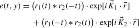
Grating G 2 performs the transformation of the temporal spectral function on back focal plane of lens L2 into temporal function. Neglecting the constant coefficients, the time domain response corresponding to the interference terms in (17) is as follows:

where \(\vec{K}_{1} = \vec{k}_{t} - \vec{k}_{r} + \vec{k}_{s}\) and \(\vec{K}_{2} = \vec{k}_{t} + \vec{k}_{r} - \vec{k}_{s}\) represent propagation vectors of two output pulses; \(\vec{k}_{s},\vec{k}_{r}\) and \(\vec{k}_{t}\) are propagation vectors of signal, reference and test pulses. * denotes convolution.
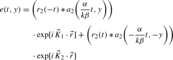
The output response is determined by \(a_{i}( - \frac{\alpha}{k\beta} t,y)\) and r i (t) (i=1,2,3). From the former definition, we know a i (x,y) represents spatial distributions of the recording and readout pulses. a i (x,y) changing into \(a_{i}( - \frac{\alpha}{ k\beta} t,y)\) means each line of the spatial image is transformed into a temporal waveform, and \(a_{i}( - \frac{\alpha}{k\beta} t,y)\) is the space-to-time conversion operator. Linear phase term \(\exp(i\frac{x_{0}}{\lambda fk\beta} t)\) represents a frequency shift, which means lateral movement of the slit on the spectral plane will tune the output optical frequency while leaving the intensity profile of the output waveform unaffected.
Equation (19) shows that a slit filter on the spectral plane can convert the spatial term of the input pulse into temporal term of the output pulse. The changed temporal term will have influence on the temporal output. Therefore, we realize the information conversion from spatial domain to temporal domain, or parallel to serial.
5 Discussions and applications
Further discussion of (19) is as listed in the following.
-
(1)
If spatial widths of the three pulses and the temporal durations of the reference pulse and test pulse are short, that is, a 1(x,y)r 1(t)=δ(x,y)δ(t), a 3(x,y)r 3(t)=δ(x,y)δ(t) and a 2(x,y)=δ(x,y), (19) is simplified to
$$ e(t,y) = r_{2}( - t)\exp [i\vec{K}_{1}\cdot\vec{r} ] + r_{2}(t)\exp [i\vec{K}_{2}\cdot\vec{r} ] $$(20)Equation (20) shows that the position of the slit has no effect on the output. The output field distribution contains a real copy and a time-reversed reconstruction of the signal wave time packet.
-
(2)
If spatial width of the three pulses and the temporal duration of the test pulse are short, (19) changes to
 (21)
(21)The convolution of two signals can be used in pulse recognition and communication.
-
(3)
If durations and widths of the reference and test pulse are short enough, (19) changes to
 (22)
(22)


The output response is a scaled representation of the input spatial profile convolved with the input temporal distribution. Assume the spatial distribution of the signal pulse is shaped and represents an image of letter “A” on the xy plane, which is located between x=10 to 40 mm and y=10 to 22.5 mm. The temporal distribution of the signal is a Gaussian function, the convolved output field distribution in direction K 2 is simulated. In simulation, assuming the input pulse is T=100 fs and the scaled factor \(\frac{\alpha}{ k\beta}\) is 1, the 3D simulation is shown Fig. 3. From Fig. 3, we can see there is no space–time conversion on axis y, the reason being that the grating and the slit have no effect on the distribution along y axis. Clearly, the input letter ‘A’ can be distinguished, with every original image pixel represented by a short pulse now and the entire input image is replaced by an ultrashort serial bit sequences. Moreover, when the duration of the pulse is shorter, the dense of the output pulses increases. The reason is that the sampling numbers increase when the duration of the pulse is shorter.

The diagram of the readout image in K 2 direction
As another application of our scheme, we discuss the generation of sequences of femtosecond pulses at very high repetition rates. Ultrafast pulse sequences are critical to the implementation of optical code division multiple access (O-CDMA) and optically assisted Internet routing networks. Among the different approaches that are used to generate fixed or arbitrary output optical waveforms the direct space-to-time (DST) pulse shapers (PSs) are of particular importance. Here we will show it can be realized by our modified spectral holography structure. In (22), if the spatial distribution of the signal pulse is shaped and represents by a rectangular function, the output response in 2D is shown in Fig. 4. Pulses with the same amplitude and duration are produced. The repetition rate of the pulse sequence is inversely proportional to the FWHM.

Output of the pulse sequence by modified spectral holography structure
6 Conclusion
By adding a slit filter, we proposed a modified spectral holography structure to perform space-to-time or parallel-to-serial conversion. Then we have deduced the recording and readout of spectral holography by femtosecond pulse with both the spatial and temporal information. The method raises the possibility of using spectral holography to acquire high-rate temporal pulse sequences, which is useful in time-division multiplexing in high-speed fiber-optic communication applications. Such space-to-time conversion has potential applications in image processing, femtosecond pulse shaping, temporal pattern generation and high speed all-optical data processing.
References
A.M. Weiner, Prog. Quantum Electron. 19, 161 (1995)
A.M. Weiner, A.M. Kan’an, IEEE J. Sel. Top. Quantum Electron. 4, 317 (1998)
Y.T. Mazurenko, Appl. Phys. B, Lasers Opt. 50, 101 (1990)
A.M. Weiner, D.E. Leaird, Opt. Lett. 19, 123 (1994)
A.M. Weiner, D.E. Leaird, D.H. Reitze, E.G. Paek, IEEE J. Quantum Electron. 28, 2251 (1992)
A.M. Weiner, D.E. Leaird, D.H. Reitze, E.G. Paek, Opt. Lett. 17, 224 (1992)
K. Ema, M. Kuwata-Gonokami, F. Shimizu, Appl. Phys. Lett. 59, 2799 (1991)
J. Ishi, H. Kunugita, K. Ema, T. Ban, T. Kondo, Appl. Phys. Lett. 77, 3487 (2000)
M.C. Nuss, M. Li, T.H. Chiu, A.M. Weiner, A. Partovi, Opt. Lett. 19, 664 (1994)
P.C. Sun, Y.T. Mazurenko, W.S.C. Chang, P.K.L. Yu, Y. Fainmann, Opt. Lett. 20, 1728 (1995)
J.-H. Chung, A.M. Weiner, J. Lightwave Technol. 21, 3323 (2003)
A.M. Kan’an, A.M. Weiner, J. Opt. Soc. Am. B 15, 1242 (1998)
D. Shayovitz, D. Marom, Opt. Lett. 36, 1957 (2011)
P.C. Sun, Y.T. Mazurenko, Y. Fainman, J. Opt. Soc. Am. A 14, 1159 (1997)
Y. Ding, D.D. Nolte, M.R. Melloch, A.M. Weiner, Opt. Lett. 22, 1101 (1997)
K. Oba, P.C. Sun, Y.T. Mazurenko, Y. Fainman, Appl. Opt. 38, 3810 (1999)
D.M. Marom, D. Panasenko, P.C. Sun, Y. Fainman, J. Opt. Soc. Am. A 18, 448 (2001)
D.M. Marom, D. Panasenko, P.C. Sun, Y.T. Mazurenko, Y. Fainman, IEEE J. Sel. Top. Quantum Electron. 7, 683 (2001)
Y.T. Mazurenko, Opt. Eng. 31, 739 (1992)
M.C. Nuss, R.L. Morrison, Opt. Lett. 20, 740 (1995)
Y. Ding, D.D. Nolte, M.R. Melloch, A.M. Weiner, IEEE J. Sel. Top. Quantum Electron. 4, 332 (1998)
D.M. Marom, P.-C. Sun, Y. Fainman, Appl. Opt. 37, 2858 (1998)
D.M. Marom, D. Panasenko, P.C. Sun, Y. Fainmann, Opt. Lett. 24, 563 (1999)
D.M. Marom, D. Panasenko, P.C. Sun, Y. Fainmann, J. Opt. Soc. Am. B 17, 1759 (2000)
D.E. Leaird, A.M. Weiner, IEEE J. Quantum Electron. 37, 494 (2001)
D.E. Leaird, A.M. Weiner, S. Shen, A. Sugita, S. Kamei, M. Ishii, K. Okamoto, Opt. Quantum Electron. 33, 811 (2001)
H. Tanabe, F. Kannari, Opt. Rev. 9, 100 (2002)
J.D. McKinney, D.-S. Seo, A.M. Weiner, IEEE J. Quantum Electron. 39, 1635 (2003)
A. Krishnan, L. Grave de Peralta, V. Kuryatkov, A.A. Bernussi, H. Temkin, Opt. Lett. 31, 640 (2006)
F. Frei, A. Galler, T. Feurer, J. Chem. Phys. 130, 034302 (2009)
O.E. Martinez, J. Opt. Soc. Am. B 3, 929 (1986)
Acknowledgements
Supported (partly) by national science funds (Nos. 60908007, 10974132), Shanghai Leading Academic Discipline Project (No. S30105)] and Shanghai Municipal Education Commission Innovation Project (12YZ002).
Author information
Authors and Affiliations
Corresponding author
Rights and permissions
About this article
Cite this article
Yan, X., Cao, L., Dai, Y. et al. All optical parallel-to-serial conversion by modified spectral holography structure. Appl. Phys. B 108, 153–158 (2012). https://doi.org/10.1007/s00340-012-5078-6
Received:
Revised:
Published:
Issue Date:
DOI: https://doi.org/10.1007/s00340-012-5078-6