
Abstract
It is a result by Lacey and Thiele (Ann. of Math. (2) 146(3):693–724, 1997; ibid. 149(2):475–496, 1999) that the bilinear Hilbert transform maps \(L^{p_{1}}(\mathbb{R}) \times L^{p_{2}}(\mathbb{R}) \) into \(L^{p_{3}}(\mathbb{R})\) whenever (p 1,p 2,p 3) is a Hölder tuple with p 1,p 2>1 and \(p_{3}>\frac{2}{3}\). We study the behavior of the quartile operator, which is the Walsh model for the bilinear Hilbert transform, when \(p_{3}=\frac{2}{3}\). We show that the quartile operator maps \(L^{p_{1}}(\mathbb{R}) \times L^{p_{2}}(\mathbb{R}) \) into \(L^{\frac{2}{3},\infty}(\mathbb{R})\) when p 1,p 2>1 and one component is restricted to subindicator functions. As a corollary, we derive that the quartile operator maps \(L^{p_{1}}(\mathbb{R}) \times L^{p_{2},\frac{2}{3}}(\mathbb{R}) \) into \(L^{\frac{2}{3},\infty}(\mathbb{R})\). We also provide weak type estimates and boundedness on Orlicz-Lorentz spaces near p 1=1,p 2=2 which improve, in the Walsh case, the results of Bilyk and Grafakos (J. Geom. Anal. 16 (4):563–584, 2006) and Carro et al. (J. Math. Anal. Appl. 357(2):479–497, 2009). Our main tool is the multi-frequency Calderón-Zygmund decomposition from (Nazarov et al. in Math. Res. Lett. 17(3):529–545, 2010).
1 The Walsh Phase Plane and the Quartile Operator
1.1 The Walsh Phase Plane
Let
be the Walsh system on [0,1]. We have written n=∑ k≥0 ε k 2k in binary representation, that is, ε k ∈{0,1}. The system {W n :n≥0} is an orthonormal basis of L 2(0,1).
We will denote by \(\mathcal{D}\) the standard dyadic grid on \(\mathbb{R}\), and write ℓ(I) for the left endpoint of a dyadic interval I. A tile \(s=I_{s} \times\omega_{s} \subset \mathbb{R}\times \mathbb{R}_{+}\) is a dyadic rectangle of area 1, that is, I s and ω s both belong to \(\mathcal{D}\) and |I s ||ω s |=1 . We define the corresponding Walsh wave packet
Let Ti be the set of all tiles. It is immediate to see that ∥w s ∥2=1 for all s∈Ti. Also, the following fundamental orthogonality property holds:
A quartile s=I s ×ω s is a dyadic rectangle with |ω s |=4|I s |−1. We think of ω s as the union of its dyadic grandchildren \(\omega _{s_{j}}\), j=1,…,4, with \(\ell(\omega_{s_{1}})< \cdots<\ell (\omega _{s_{4}})\), and denote by s j the tiles \(I_{s} \times\omega_{s_{j}}\), which we call frequency grandchildren of s. The set of all quartiles will be denoted by Qt.
1.2 The Quartile Operator
We define the quartile operator
and the associated trilinear form

where S⊂Qt is an arbitrary collection of quartiles. The quartile operator has been introduced in [12] (see also [14]) as a discrete model for the bilinear Hilbert transform
Hereafter, \(f^{*}:\mathbb{R}^{+} \to[0,\infty)\) indicates the decreasing rearrangement of f, and for 0<p,q≤∞, p≠∞, we denote by \(L^{p,q}(\mathbb{R})\) the Lorentz space with norm (or quasi-norm if either p or q are less than 1)
Let (p 1,p 2,p 3)∈(0,∞]3 be a Hölder tuple of exponents, that is
A dilation-invariance argument shows that if p i ,q i ∈(0,∞], i=1,2,3 are tuples of exponents such that
then necessarily (p 1,p 2,p 3) is a Hölder tuple. It is a celebrated result by Lacey and Thiele [7, 8] that
whenever (p 1,p 2,p 3) is a Hölder tuple with p 1,p 2>1 and \(p_{3}>\frac{2}{3}\). Their proof uses the fact that BHT is an average of Fourier analogues of V Qt (where the Walsh wave packets are replaced by certain “Fourier wave packets”) that are uniformly bounded. The analysis of Walsh model sums is technically simpler than the one of their Fourier counterparts (in part due to (1.1)), but it generally preserves the main conceptual difficulties from the Fourier world. Due to this, the “Walsh case” is the ideal scenario for conveying new ideas in the most transparent way.
The quartile operator shares the same Hölder scaling property exhibited by BHT and is known to be bounded in the same range of exponents, [12]. A counterexample by Lacey and Thiele [8], see [9] for details, shows that having \(p_{3}\geq\frac{2}{3}\) is necessary in order for bounds of the type (1.4) to hold true for (the Fourier analogue of) V Qt .
The main purpose of the present paper is the investigation of the endpoint behavior of V Qt . It is natural to conjecture
Conjecture 1
For each p 1,p 2>1 such that \(\frac{1}{p_{1}} + \frac {1}{p_{2}} = \frac{3}{2}\) we have
We expect the same bound to hold for BHT. To support the conjecture we mention that there is no known counterexample to disprove even the strong type bound
1.3 A Summary of Previous Results
Perhaps the simplest way to prove (1.5) is to establish the so called generalized restricted type bounds of the form

where \(F_{3}' \subset F_{3}\) is an appropriately chosen major set, for all tuples (α 1,α 2,α 3) satisfying
Here and in what follows, the term major set indicates any subset F′⊂F of a set F of finite measure with \(|F'| \geq \frac{1}{8} |F|\). These estimates are then turned into strong type bounds via interpolation.
We also mention some partial results towards Conjecture 1. A refinement of the proof by Lacey and Thiele by Bilyk and Grafakos [3] provides the following logarithmically bumped up version of (1.7) near the endpoint tuple \((1,\frac{1}{2},-\frac{1}{2})\):

for functions \(|f_{1}| \leq \mathbf {1}_{F_{1}}, \,|f_{2}| \leq \mathbf {1}_{F_{2}},\, |f_{3}| \leq \mathbf {1}_{F_{3}'}\), in the regime (say) |F 1|≤|F 2|. The analogous estimate for BHT is in turn used to derive distributional estimates, and, in the subsequent work [5], to derive estimates on Lorentz and Orlicz-Lorentz spaces near the endpoint \(p_{3}= \frac{2}{3}\).
2 Main Results
We now detail our first main theorem, which is a weak \(L^{\frac{2}{3}}\) bound with only one subindicator function.
Theorem 2
Let p 1,p 2>1, \(\textstyle\frac {1}{p_{1}}+ \frac{1}{p_{2}}= \frac{3}{2}\). Then we have the mixed type estimate
Theorem 2 is a fairly direct consequence of the proposition below, which is of independent interest. Indeed, it is worth mentioning that the generalized restricted type estimate (1.7) was only known to hold in the open range \(\alpha_{3}> -\frac{1}{2}\). This is because—in the terminology of the following sections—the summation of the forests gives rise to a lacunary series that diverges when \(\alpha_{3}= -\frac{1}{2}\). The following proposition implies the endpoint \(\alpha_{3}= -\frac{1}{2}\) generalized restricted type (1.7), but in fact it is stronger than that. The proof will be carried out in Sect. 5; we kept track of the explicit dependence on p 1 of the implied constant in the estimate (2.2).
Proposition 2.1
Let p 1,p 2>1, \(\textstyle\frac{1}{p_{1}}+ \frac{1}{p_{2}}= \frac{3}{2}\). Then for every \(f_{1} \in L^{p_{1}}(\mathbb{R})\) and every \(F_{2}, G_{3} \subset \mathbb{R}\), there exists a major set F 3⊂G 3 such that

Proof that Proposition 2.1 implies Theorem 2
Let f
1,F
2, f
2 with \(|f_{2}| \leq \mathbf {1}_{F_{2}} \) be given. By using a standard approximation argument, it suffices to prove the bound for an arbitrary finite subset S⊂Qt, as long as the bound is independent of S. Since S is a finite collection, there exists a constant C
0, possibly depending on p
1,S,f
1, and f
2, such that (2.1) holds. We show that the constant is independent of all but p
1. Fix λ>0 and take G
3 to be the set in the left hand side of (2.1). The existence of C
0 implies that G
3 has finite measure, so that we may apply Proposition 2.1, and obtain the existence of a major set F
3⊂G
3 such that (2.2) holds for any f
3 with \(|f_{3}| \leq \mathbf {1}_{F_{3}} \). We can choose f
3 such that  , so that

which, rearranged, gives exactly (2.1). □
We are interested in extrapolating the bound of Theorem 2 to Lorentz spaces. In this direction we have the theorem below, which can be seen as a partial result towards the conjectured bound (1.6). We next show how this follows from Theorem 2, via linear extrapolation in the style of [4].
Theorem 3
Let p 1,p 2>1, \(\textstyle\frac {1}{p_{1}}+ \frac{1}{p_{2}}= \frac{3}{2}\). Then
Remark 2.2
Note that \({L^{p_{2},\frac{2}{3}}(\mathbb{R})}\) is a proper subspace of \({L^{p_{2}} (\mathbb{R})}\); the result of Theorem 3 is therefore a strictly weaker version of (1.6).
Proof that Theorem 2 implies Theorem 3
We can normalize \(\|f_{1}\|_{p_{1}} =1 = \|f_{2} \|_{{p_{2},\frac{2}{3}}}\). We perform the well-known decomposition
with each G k being a bounded set and
We then have

Applying Theorem 2, we obtain the estimate
It is shown in [4, Theorem 3.1] (see also [5, Theorem 2.1]) that
Therefore, taking advantage of (2.5) and subsequently of (2.4),
and this completes the proof. □
Theorems 2 and 3 do not cover the case p 1=1,p 2=2. In this subsection, we derive endpoint results involving Orlicz-Lorentz substitutes of \(L^{1}(\mathbb{R})\) and \(L^{\frac{2}{3},\infty}(\mathbb{R})\) as a consequence of the estimate

Let us show how to obtain (2.6) from the (family of) weak type estimates contained in the following proposition, whose proof we defer to Sect. 5.
Proposition 2.3
Let 1<p<2, and r defined by \(\frac{1}{p}+\frac{1}{2}=\frac{1}{r}\). Then \(\|\mathsf{V}_{\mathbf{Qt}}\|_{L^{p} \times L^{2} \to L^{r,\infty}} \lesssim p'\), that is
Note that, for any given 1<p<2, (2.7) can be rewritten in terms of the decreasing rearrangement V(t):=(V Qt (f 1,f 2))∗(t) as
Since ∥f 1∥∞≤1, we can estimate \(\|f_{1}\|_{p}\leq\|f_{1}\| _{1}^{\frac{1}{p}}\) in each instance of (2.8). This yields
At this point, (2.6) follows by taking infimum over 1<p<2 in the above inequality.
Remark 2.4
In the literature, it is often the case that estimates in the vein of (2.6) are derived by first establishing the weaker version where one or both functions f 1,f 2 are restricted to be subindicator. This restriction is then lifted by using further properties of the (multi)-sublinear operator (e.g. ε-δ atomic approximability). This is the approach adopted in [5] for the bilinear Hilbert transform and by Antonov [1] and Arias de Reyna [2] for the Carleson maximal partial Fourier sum operator. Our own approach of extrapolating from weak type estimates (like (2.7)), as opposed to restricted weak type estimates as usual, bypasses the above additional step.
As in [5], we introduce the weak type weighted Lorentz space X with quasi-norm
The space X is a logarithmic enlargement of \(L^{\frac{2}{3}, \infty}\). Note that an application of the trivial inequality \(\frac{1}{2}\log(\mathrm{e}+ab) \leq\log(\mathrm{e}+ a)\log(\mathrm{e}+b)\) for all a,b>0, turns (2.6), after rearranging and taking supremum over t>0, into
The above estimate (2.9) can be coupled with linear extrapolation in the first function f 1 to obtain the two endpoint theorems below.
Theorem 4
There holds
where \(L^{1,\frac{2}{3}} \log L^{ \frac{2}{3}}(\mathbb{R}) \) is the Lorentz-Orlicz quasi-Banach space with quasinorm
Theorem 5
We have that, for each ε>0,
where \(L \log L (\log\log L)^{\frac{1}{2}} (\log\log\log L)^{\frac{1}{2}+\varepsilon }(\mathbb{R}) \) is the Orlicz space Footnote 1 with Orlicz function
Theorem 4 is obtained by fixing f 2 with ∥f 2∥2=1 and straightforwardly applying the linear extrapolation theorem [5, Theorem 2.1(b)] to the linear operator f 1↦V Qt (f 1,f 2), in view of estimate (2.9). Even the weaker version of (2.9) where f 1 is taken to be a subindicator function would comply with the assumption thereof. Theorem 5 follows from (the full strength of) (2.9) via the level set decomposition argument of [5, Example 3.12], again applied to the linear operator f 1↦V Qt (f 1,f 2).
Remark 2.5
Theorems 4 and 5 improve respectively the bounds

proven in Sect. 4.1 of [5] (when restricted to the Walsh case). In particular, we can always take one function in \(L^{2}(\mathbb{R})\). We also stress that (2.9) allows us to freeze the L 2 function and only employ linear extrapolation results to derive our Theorems 4 and 5, in contrast with the approach of [5] where bilinear extrapolation is needed. Finally, it is easy to see that the two substitutes for \(L^{1}(\mathbb{R})\) in Theorems 4 and 5 are not comparable; thus none of the two results can be obtained from the other.
Remark 2.6
One might be interested in finding an Orlicz-Lorentz modification of the pair \(L^{1}(\mathbb{R}) \times L^{2}(\mathbb{R})\) which is mapped by V Qt into \(L^{\frac{2}{3}, \infty} (\mathbb{R})\) (strictly smaller than the space X appearing in Theorems 4 and 5). This can be done by means of the following restricted weak type estimate: given any two sets \(F_{1},F_{2} \subset \mathbb{R}\) with |F 1|≤|F 2|,
for all \(|f_{1}|\leq \mathbf {1}_{F_{1}}, \; |f_{2}|\leq \mathbf {1}_{F_{2}}\); estimate (2.10) is obtained by applying (2.1) with the optimal choice of p 1,p 2 given by \((p_{1})'= \log (\mathrm{e}+ \textstyle\frac{|F_{2}|}{|F_{1}|} )\). Then an application of the multilinear extrapolation Theorem 2.6 in [5], yields the bound
3 Analysis and Combinatorics in the Walsh Phase Plane
We refer to [12, 14] for more details about the results in this section.
Let us introduce some more notation. To simplify the combinatorial arguments, it is convenient to split Qt into two subsets Qt 1, Qt 2 such that
For the rest of the paper we will assume to be working with finite collections of quartiles S⊂Qt 1.
As described in the introductory section, we denote by s j the tiles \(I_{s} \times\omega_{s_{j}}\), which we call frequency grandchildren of s. Symmetrically, we will denote by s j, j=1,…,4 the tiles \(I_{s}^{j} \times\omega_{s}\), where \(I_{s}^{j}\) are the four dyadic grandchildren of I s , and will refer to them as spatial grandchildren of s. Finally, we use the notations
and
for the shadow of a set of tiles (or quartiles) S in the phase plane.
3.1 Trees and Phase Space Projection
We will use the well-known Fefferman order relation on quartiles:
Note that, as a consequence of (1.1), if two quartiles s,s′ are not related under ≪ then
A collection S⊂Qt 1 is called convex if
We will use repeatedly that the intersection of two convex sets is convex.
A collection of quartiles T⊂Qt 1 is called tree with top quartile s T ∈Qt 1 if s≪s T for all s∈T. We use the notation \(I_{\mathbf{T}}:=I_{s_{\mathbf{T}}}, \omega_{\mathbf{T}}=\omega _{s_{\mathbf{T}}}\). We say that a tree T is a j-tree (for some j∈{1,…,4}) if \(\omega_{\mathbf{T}} \subset\omega_{s_{j}}\) for all s∈T∖{s T }. Note that if T is a j-tree the tiles {s k :k∈{1,…,4}∖{j},s∈T} are pairwise disjoint.
If S is a finite collection of pairwise disjoint tiles, define
as a subspace of \(L^{2}(\mathbb{R})\).
The lemma below is geared towards the subsequent definition of the phase-space projection Π T associated to a convex j-tree T.
Lemma 3.1
Let T be a finite, convex j-tree, with j∈{1,…,4}. Then there exists a finite set of pairwise disjoint tiles \(\mathbf{T}' \subset \mathbf{T}_{\star}^{\star}\) such that sh(T)=sh(T′) and with the further property
Proof
We proceed by induction on the number of quartiles. The base case #T=1 is trivially true. Let now T be a given finite convex 1-tree (to fix ideas). Choose a minimal (with respect to ≪) quartile s∈T. Then \(\dot{\mathbf{T}}:=\mathbf{T}\backslash\{s\}\) is a convex 1-tree. By induction assumption, we find a collection of pairwise disjoint tiles \(\dot{\mathbf{T}}' \subset\dot{\mathbf{T}}^{\star}_{\star}\) with \(\mathsf{sh}(\dot{\mathbf{T}}')=\mathsf{sh}(\dot{\mathbf{T}})\) and such that (3.4) holds. Let I be the unique interval in \(\{I_{s'}: s' \in\dot{\mathbf{T}}'\}\) such that I s ⊆̷I. Since \(\dot{\mathbf{T}}\) is a convex 1-tree, there exists a unique quartile \(\sigma\in\dot{\mathbf{T}}\) such that I σ =I and |I σ |=4|I s |. Moreover \(\omega_{s_{1}} =\omega_{\sigma}\). Setting
we see that sh(T′)=sh(T) and that T′ satisfies (3.4). The induction is complete. □
For a finite convex j-tree T, let T′ be the corresponding collection of pairwise disjoint tiles given by Lemma 3.1. The wave packets {w s :s∈T′} are an orthonormal basis of H T′, due to the corresponding tiles in T′ being pairwise disjoint. Thus the orthogonal projection \(\varPi _{\mathbf{T}}:L^{2}(\mathbb{R}) \to H_{\mathbf{T}'}\) can be written as
In particular, if s is a quartile, then
Lemma 3.2
Let T be a convex j-tree. We have the equality
Proof
This follows immediately from the fact that \(s \in \mathbf{T}^{\star}_{\star}\) implies w s ∈H T′. In turn, this is a consequence of the recursion relation for Walsh wave packets. See [14, Corollary 1.10]. □
4 Sizes, Trees and Single Tree Estimates
For an interval \(I \subset \mathbb{R}\), we adopt the notation
Accordingly, we define the dyadic maximal functions
Let \(f \in L^{2}(\mathbb{R})\) and let S be a set of quartiles. We set
Note that
It is immediate to see that
Lemma 4.1
Let T be a convex tree, j=1,…,4, and \(\mathbf{T}_{j} =\{ s \in \mathbf{T}: \omega_{s_{j}} \supseteq\omega_{s_{\mathbf{T}}} \}\). We have the John-Nirenberg type inequality
Proof
Since \(\varPi _{\mathbf{T}_{j}} f\) is supported on I T , it suffices to show that
Note that T j is also a convex tree. Fix x∈I T . Due to (3.4), we have that x∈I s for at most four tiles s∈(T j )′. Thus
as claimed. The lemma follows. □
The John-Nirenberg inequality above is all we need to produce an estimate on the trilinear form (1.2) restricted to a tree.
Lemma 4.2
Let T be a convex tree. Then

Proof
We argue separately for each \(\mathbf{T}_{j}=\{s \in \mathbf{T}: \omega_{\mathbf{T}} \subset \omega_{s_{j}}\} \). The argument for s T is even simpler. Assume j=1 for simplicity. We have

We have used that \(\{w_{s_{j}}: s\in \mathbf{T}_{1}\}\) is an orthonormal set for j=2,3, since the corresponding tiles {s j :s∈T 1} are pairwise disjoint, and (4.4) to conclude. □
A collection of quartiles S is called a forest if S can be partitioned in (pairwise disjoint) convex trees \(\{\mathbf{T}: \mathbf{T}\in \mathcal{F}\}\). It may be that a given S may admit many such partitions \(\mathcal{F}\). We define
The next lemma skims the trees with large relative size off the collection S, organizing them into a forest.
Lemma 4.3
Let S be a finite convex collection of quartiles with size f (S)≤σ. Then S=S hi ∪S lo , such that
-
both S lo and S hi are convex;
-
\(\mathrm{size}_{f}(\mathbf{S}_{\mathsf{lo}} )\leq\frac{\sigma}{2}\);
-
S hi is a forest with \(\mathrm{tops}( \mathbf{S}_{\mathsf{hi}}) \lesssim\sigma^{-2}\|f\|^{2}_{2} \).
Proof
This is a recursive procedure. Set S stock :=S. Select a maximal (with respect to ≪) quartile t∈S stock such that
Define
and note that since S stock is convex, T(t) is a convex tree. Add T(t) to the family \(\mathcal{F}\). Reset the new value S stock :=S stock ∖{s:s∈T(t)}, and restart the procedure.
The algorithm is over when there is no t to be selected. Then define S hi to consist of the union of all the selected trees in \(\mathcal{F}\), and S lo =S∖S hi .
The first two needed properties are easy to check. By maximality the selected quartiles t are pairwise disjoint, and thus the functions Π t f are pairwise orthogonal, thanks to (1.1). It follows that
□
We will decompose the model sum (1.2) by organizing the quartiles of S into forests of definite size. The lemma below turns the tree estimate (4.5) into a forest estimate.
Lemma 4.4
Let S be a finite convex collection of quartiles which is also a forest, with
Then

Proof
Choose the minimizing forest \(\mathcal{F}\) and write
Let \(n_{0}= -2\log (\frac{\sigma_{2}\|f_{1}\|_{2}}{\|f_{2}\|_{2}} )\). If \(\sigma_{1} \sigma_{2}^{-1} \|f_{2}\|_{2} \leq\|f_{1}\|_{2} \), in other words if \(\mathrm{size}_{f_{1}}(\mathbf{S})\le2^{-\frac{n_{0}}{2}}\), then use the single tree estimate (4.5) to get

Otherwise, we have \(\sigma_{1} \geq2^{-\frac{n_{0}}{2}}\). We iteratively apply Lemma 4.3 with respect to f 1, a finite number of times, and write

Note that we also continue to have
Then, using triangle inequality, (4.5) again, and summing up,

as claimed. To deal with the contribution from \(\tilde{\mathbf{S}}\), redo the computations from the first case, this time with \(\mathbf{S}:=\tilde{\mathbf{S}}\). Lemma 4.3 guarantees \(\tilde{\mathbf{S}}\) is convex. To see that it is a forest, note that it is the disjoint union of the convex trees \(\tilde {\mathbf{T}}:=\mathbf{T}\cap\tilde{\mathbf{S}}\), with \(\mathbf{T}\in \mathcal{F}\), each of which is assigned the same top as T. It is then obvious that \(\mathrm{tops}(\tilde{\mathbf{S}})\le \mathrm{tops}(\mathbf{S})\). □
5 Proofs of Propositions 2.1 and 2.3
We first prove Proposition 2.1, and then indicate the necessary changes for Proposition 2.3 at the end of the section. In this proof, we use the notation (p 1)′=:q.
5.1 Reductions
By a limiting argument, it will suffice to replace Qt 1 with a finite convex subset S. The constants implied by the almost inequality signs are not allowed to depend on p 1, S or f 1,f 2,f 3. Recall that we have the separation of scales (3.1) for S. We show how (2.2) follows from

whenever 1≤|G 3|<4, which we summarize as |G 3|∼1 below.
Indeed, if λ is a power of 4 chosen to have \(|\tilde{G_{3}}:= \{ \lambda^{-1}x: x \in G_{3}\}|\sim1\), then \(|\tilde{F_{2}}:=\{\lambda ^{-1}x: x \in F_{2}\}| \sim|G_{3}|^{-1}|F_{2}|\). Observe that S λ ={s λ =λ −1 I s ×λω s :s∈S} is still a convex subset of Qt 1. If we employ (5.1), we get the existence of \(\tilde{F_{3}} \subset\tilde{G_{3}}\), with \(|\tilde {F_{3}}|\geq\frac{1}{8} |\tilde{G_{3}}|\) and

It follows that \(F_{3} =\{\lambda y: y \in\tilde{F_{3}}\} \subset G_{3}\) is major in G 3. Since by dilation invariance

(2.2) follows by combining (5.2) with the last display.
We perform two more reductions. First, by linearity in the first function, it is enough to prove the case \(\|f_{1}\|_{p_{1}}=1\) of (5.1). Furthermore, we can assume |F 2|≤|G 3|<4. Indeed, if |F 2|≥|G 3|≥1 instead, we take r>p 2: since the tuple \((\frac{1}{p_{1}},\frac{1}{r},1-\frac{1}{p_{1}}-\frac{1}{r} )\) belongs to the range (1.8) we apply the bound (1.5) (which holds for the discrete model Q S as well), and get

which is stronger than (2.2) in the region |F 2|≥1. The dependence on p 1 of the constant in the above inequality follows easily if one tracks it down in the usual proof, given for instance (in the Fourier case) in Chap. 6 of [13].
Summarizing, we have reduced to proving the following statement: show that for all f 1 of unit norm in \(L^{p_{1}}(\mathbb{R})\), \(F_{2} \subset \mathbb{R}\), |F 2|≤4, \(G_{3}\subset \mathbb{R}\) with |G 3|∼1, there exists a major subset F 3⊂G 3 with

5.2 Exceptional Sets
We define the exceptional sets
For an appropriate choice of the constant c
Set F 3:=G 3∖(E 1∪E 2); by the above, \(|F_{3}| \geq \frac{1}{2} \geq\frac{1}{8} |G_{3}|\). We note that when \(|f_{3}|\leq \mathbf {1}_{F_{3}}\),

Therefore we will just replace S by S good in what follows. Thus, by construction, in view of the upper bound (4.3),
The last bound is a consequence of f 3 being uniformly bounded by 1.
5.3 A Multi-frequency Calderón-Zygmund Decomposition
Before we proceed with the proof, we present an abstract lemma which involves a multi-frequency Calderón Zygmund decomposition. This decomposition was proved in [10] for the Fourier case, and has since then been successfully used in getting uniform estimates for the quartile operator [11] and getting bounds for the Walsh version of the lacunary Carleson’s operator near L 1 [6]. Our lemma is essentially contained in [11].
Lemma 5.1
Let 1<p 1<2 , q=(p 1)′ and \(\|f_{1}\| _{p_{1}}=1\). Define \(\alpha=1 -\frac{2}{q}\) and let S be a finite forest with tops(S)≤A 2 for some A≥1. Then there exists \(g_{1}^{\mathbf{S}}\) such that

Proof
Choose a minimizing \(\mathcal{F}\) and define the counting function \(N =\sum_{\mathbf{T}\in \mathcal{F}} \mathbf {1}_{I_{\mathbf{T}}}\). Let I∈I be the collection of the children of the maximal dyadic intervals inside \(E_{1}= \{\mathsf{M}_{p_{1}} f_{1}\ge c\}\). The intervals I are pairwise disjoint, and
Note also that, as a consequence of (5.7),
where I ∗ is the dyadic parent of I. This implies that the counting function N is constant equal to N I on I. We introduce the collection of tiles for each I∈I
Observe that if s∈S I and s′ is a quartile in S with \(s\ll s'_{1}\), then \(s \ll s'_{j} \) for j=2,…,4 too. This is because |I s′|≥4|I|, by the above observations. As a first consequence, \(w_{s'_{j}}\) is a scalar multiple of w s on I, and in particular
As a further consequence, #S I ≤N I , since each ω s with s∈S I contains the frequency component of some of the N I trees whose top spatial interval contains I. Let \(v=\sum_{s \in \mathbf{S}_{I}} a_{s} w_{s} \in H_{\mathbf{S}_{I}}\). We see that, for all q≥2,

With this observation and the second half of (5.9),
By the Riesz representation theorem, we get the existence of \(g_{I} \in H_{\mathbf{S}_{I}}\), with
We set
In particular, \(g_{1}^{\mathbf{S}}=f_{1}\) outside of E 1. Thus, for every s∈S, j=1,…,4, in view of (5.10)

and it follows immediately that

Since |f 1|≲1 on \(E_{1}^{c}\) and p 1<2,
while

In the last step, we have used the bound on the sum of the |I|. Collecting (5.13)–(5.15), we are done. □
5.4 Proof of (5.4)
Iterating the size Lemma 4.3 with respect to f 2 and f 3 and then intersecting the forests, and recalling (5.8), we decompose
with each \(\mathbf{S}_{n_{2},n_{3}}\) being a convex forest such that
We use Lemma 5.1 for each \(\mathbf{S}_{n_{2},n_{3}}\), obtaining functions \(g_{1}^{\mathbf{S}_{n_{2},n_{3}}}\) satisfying
and

Recall here that \(\alpha= 1-\frac{2}{q}\). Applying (4.7) of Lemma 4.4 (or the analogous estimate where 2 and 3 are permuted), we obtain the forest estimates

We used that \(\|f_{2}\|_{2} \leq|F_{2}|^{\frac{1}{2}} \) and \(\|f_{3}\|_{2} \leq |F_{3}|^{\frac{1}{2}}\sim1\). We now use the triangle inequality over the forests \(\mathbf{S}_{n_{2},n_{3}}\). This yields the estimate

We split the above sum into two separate regimes.
-
Regime \(R_{2}=\{2^{-n_{2}} \leq |F_{2}|^{\frac{1}{2}}, 1 \leq2^{n_{3}} \leq2^{n_{2}}\}\).
We use the second forest estimate in (5.18), and obtain

Here we used that
$$ \sum_{n \geq n_0} 2^{-(1-\alpha) n} \sim\frac{1}{1-\alpha} 2^{-(1-\alpha) n_0} \sim q |F_2|^{\frac{1}{q}}, $$(5.20)for \(n_{0} = -\frac{1}{2} \log|F_{2}|\) and that
$$ \frac{1}{2}+ \frac{1}{q} = \frac{3}{2} -\frac{1}{p_1}= \frac{1}{p_2}. $$(5.21) -
Regime \(R_{3}=\{ |F_{2}|^{-\frac{1}{2}} \leq2^{n_{2}} \leq2^{n_{3}}\}\).
We use the first forest estimate in (5.18), and get
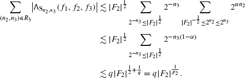
Combining the last two displays, we obtain exactly (5.4), and in turn, the theorem.


5.5 Proof of Proposition 2.3
By the standard argument that converts generalized restricted weak type estimates into weak type (see the proof of (2.1) given (2.2)), (2.7) follows if we show that for all subsets S⊂Qt, \(f_{1} \in L^{p}(\mathbb{R})\), \(f_{2} \in L^{2}(\mathbb{R})\), and \(G_{3}\subset \mathbb{R}\) there exists a major subset F 3⊂G 3 such that for all functions f 3 with \(|f_{3}|\leq \mathbf {1}_{F_{3}}\)

Performing the same reductions as in Sect. 5.1 (i.e. using linearity and dyadic scaling) it further suffices to assume ∥f 1∥ p =∥f 2∥2=1, 1≤|G 3|<4.
The first step is yet again eliminating the two exceptional sets
with c>0 suitably chosen, so that F 3:=G 3∖(E 1∪E 2) is a major subset of G 3. Arguing just like we did at the end of Sect. 5.2, we arrive at the following starting point for the size decomposition:
We now decompose S by means of the size lemma with respect to f 2,f 3:
with
Applying Lemma 5.1 to f 1 relatively to each collection \(\mathbf{S}_{n_{2},n_{3}}\), we get the existence of a function \(g_{1}^{\mathbf{S}_{n_{2},n_{3}}}\) with
and  . Applying Lemma 4.4, the forest estimate then becomes (denoting n
⋆:=max{n
2,n
3})
. Applying Lemma 4.4, the forest estimate then becomes (denoting n
⋆:=max{n
2,n
3})

We have tacitly used that \(\|f_{2}\|_{2}=1, \|f_{3}\|_{2}\leq|F_{3}|^{\frac{1}{2}}\lesssim1\). Finally, we use the triangle inequality to estimate

which yields (the scaled version of) (5.22) The proof of (2.7) is thus complete.
6 Concluding Remarks
There are two immediate directions for improvement of the results contained in Sect. 2. The first one is of technical nature, and consists in extending all the results here to the Fourier analogue of the quartile operator, and thus ultimately to BHT. The main difficulty lies in recasting efficiently the multi-frequency Calderón-Zygmund decomposition of Lemma 5.1 in the Fourier case: while suitable analogues of (5.11) hold true, the insertion of the phase space projection as in (5.17) creates a nontrivial error term which must be carefully estimated. We plan on dealing with this issue in a future work.
A second, probably harder and more interesting task is upgrading Theorem 3 to the full strength of the conjectured (1.6). The techniques employed here do not seem to work when both functions in (2.1) are taken to be unrestricted. This case is intrinsically more difficult, since two of the three functions in  are not in L
2 locally and thus they both need to be treated by the multi-frequency Calderón-Zygmund decomposition. A very appealing situation is the symmetric case
are not in L
2 locally and thus they both need to be treated by the multi-frequency Calderón-Zygmund decomposition. A very appealing situation is the symmetric case
To prove this bound, it will be enough to show that for any \(F\subset \mathbb{R}\) with |F|=1 and \(\|f\|_{\frac{4}{3}}=1\) there exists a major subset G of F such that

Indeed, (6.1) for arbitrary f 1,f 2 will then follow by applying (6.2) to f∈{f 1,f 2,f 1−f 2}. It is tempting to believe that (6.2) should be the easiest case since the same multi-frequency Calderón-Zygmund decomposition would simultaneously resolve both components.
Notes
Given a Young’s function φ:[0,∞]→[0,∞), the Orlicz (Banach) space \(L^{\varphi}(\mathbb{R})\) is the space of measurable functions on \(\mathbb{R}\) with finite Orlicz norm
$$\|f\|_{L^\varphi}:= \inf \biggl\{\lambda>0 : \int_\mathbb{R}\varphi \biggl(\frac{|f(x)|}{\lambda} \biggr)\, {\rm d}x \leq1 \biggr\}. $$
References
Antonov, N.Yu.: Convergence of Fourier series. In: Proceedings of the XX Workshop on Function Theory, Moscow, 1995, vol. 2, pp. 187–196 (1996). MR 1407066 (97h:42005)
Arias-de Reyna, J.: Pointwise convergence of Fourier series. J. London Math. Soc. (2) 65(1), 139–153 (2002). MR 1875141 (2002k:42009)
Bilyk, D., Grafakos, L.: Distributional estimates for the bilinear Hilbert transform. J. Geom. Anal. 16(4), 563–584 (2006). MR 2271944 (2007j:46033b)
Carro, M., Colzani, L., Sinnamon, G.: From restricted type to strong type estimates on quasi-Banach rearrangement invariant spaces. Studia Math. 182(1), 1–27 (2007). MR 2326489 (2008f:46033)
Carro, M.J., Grafakos, L., María Martell, J., Soria, F.: Multilinear extrapolation and applications to the bilinear Hilbert transform. J. Math. Anal. Appl. 357(2), 479–497 (2009). MR 2557660 (2010k:44008)
Do, Y., Lacey, M.: On the convergence of lacunary Walsh-Fourier series. Preprint, arXiv:1101.2461 [math.CA]
Lacey, M., Thiele, C.: L p estimates on the bilinear Hilbert transform for 2<p<∞. Ann. of Math. (2) 146(3), 693–724 (1997). MR 1491450 (99b:42014)
Lacey, M., Thiele, C.: On Calderón’s conjecture. Ann. of Math. (2) 149(2), 475–496 (1999). MR 1689336 (2000d:42003)
Lacey, M.T.: The bilinear maximal functions map into L p for 2/3<p≤1. Ann. of Math. (2) 151(1), 35–57 (2000). MR 1745019 (2001b:42015)
Nazarov, F., Oberlin, R., Thiele, C.: A Calderón-Zygmund decomposition for multiple frequencies and an application to an extension of a lemma of Bourgain. Math. Res. Lett. 17(3), 529–545 (2010). MR 2653686 (2011d:42047)
Oberlin, R., Thiele, C.: New uniform bounds for a Walsh model of the bilinear Hilbert transform. Preprint, arXiv:1004.4019v1 [math.CA]
Thiele, C.: The quartile operator and pointwise convergence of Walsh series. Trans. Amer. Math. Soc. 352(12), 5745–5766 (2000). MR 1695038 (2001b:42007)
Thiele, C.: Wave packet analysis. In: CBMS Regional Conference Series in Mathematics, Washington, DC, vol. 105 (2006). Published for the Conference Board of the Mathematical Sciences, MR 2199086 (2006m:42073)
Thiele, C.M.: Time-frequency analysis in the discrete phase plane. Ph.D. thesis, Yale University, ProQuest LLC, Ann Arbor, MI (1995). MR 2692998
Acknowledgements
We thank Dimitry Bilyk for valuable discussions and pointers to preexisting literature. We would also like to thank the very careful referee who has pointed out some inaccuracies in the first version of the manuscript.
Author information
Authors and Affiliations
Corresponding author
Additional information
Communicated by Loukas Grafakos.
The first author is partially supported by a Sloan Research Fellowship and by NSF Grant DMS-0901208. The second author is an INdAM—Cofund Marie Curie Fellow and is partially supported by the National Science Foundation under the grant NSF-DMS-1206438, and by the Research Fund of Indiana University.
Rights and permissions
About this article
Cite this article
Demeter, C., Di Plinio, F. Endpoint Bounds for the Quartile Operator. J Fourier Anal Appl 19, 836–856 (2013). https://doi.org/10.1007/s00041-013-9275-4
Received:
Revised:
Published:
Issue Date:
DOI: https://doi.org/10.1007/s00041-013-9275-4