New Characterizations of Besov-Triebel-Lizorkin-Hausdorff Spaces Including Coorbits and Wavelets

Abstract

In this paper, the authors establish new characterizations of the recently introduced Besov-type spaces $\dot{B}^{s,\tau}_{p,q}({\mathbb{R}}^{n})$ and Triebel-Lizorkin-type spaces $\dot{F}^{s,\tau}_{p,q}({\mathbb{R}}^{n})$ with p∈(0,∞], s∈ℝ, τ∈[0,∞), and q∈(0,∞], as well as their preduals, the Besov-Hausdorff spaces $B\!\dot{H}^{s,\tau}_{p,q}({\mathbb{R}}^{n})$ and Triebel-Lizorkin-Hausdorff spaces $F\!\dot{H}^{s,\tau}_{p,q}({\mathbb{R}}^{n})$, in terms of the local means, the Peetre maximal function of local means, and the tent space (the Lusin area function) in both discrete and continuous types. As applications, the authors then obtain interpretations as coorbits in the sense of Rauhut (Stud. Math. 180:237–253, 2007) and discretizations via biorthogonal wavelet bases for the full range of parameters of these function spaces. Even for some special cases of this setting such as $\dot{F}^{s}_{\infty,q}({\mathbb{R}}^{n})$ for s∈ℝ, q∈(0,∞] (including  BMO(ℝⁿ) when s=0 and q=2), the Q space Q _α (ℝⁿ), the Hardy-Hausdorff space HH _−α (ℝⁿ) for α∈(0,min{n/2,1}), the Morrey space ${\mathcal{M}}^{u}_{p}({\mathbb{R}}^{n})$ for 1<p≤u<∞, and the Triebel-Lizorkin-Morrey space $\dot{\mathcal{E}}^{s}_{upq}({\mathbb{R}}^{n})$ for 0<p≤u<∞, s∈ℝ and q∈(0,∞], some of these results are new.

1 Introduction

In the last few decades, function spaces have been one of the central topics in modern harmonic analysis, and are widely used in various areas such as the potential theory, partial differential equations, and the approximation theory. The Besov-type space ${\dot {B}_{p,q}^{s,\tau }({{{\mathbb{R}}}^{n}})}$, the Triebel-Lizorkin-type space ${\dot {F}_{p,q}^{s,\tau }({{{\mathbb{R}}}^{n}})}$, and their preduals, the Besov-Hausdorff space ${B\!\dot {H}_{p,q}^{s,\tau }({{{\mathbb{R}}}^{n}})}$ and Triebel-Lizorkin-Hausdorff space ${F\!\dot {H}_{p,q}^{s,\tau }({{{\mathbb{R}}}^{n}})}$ were recently introduced and investigated in [43, 57, 58, 61, 62]. These spaces establish the connection between the classical Besov-Triebel-Lizorkin spaces (see, for example, [22, 47, 49]), the Q spaces in [17], and the Hardy-Hausdorff spaces in [15], which has been posed as an open question in [15]. It was shown in [43, 57, 58] that these spaces unify and generalize many classical function spaces including classical Besov and Triebel-Lizorkin spaces, Triebel-Lizorkin-Morrey spaces (see, for example, [41–43, 51]), Q spaces, and Hardy-Hausdorff spaces (see also [54, 55]).

These spaces are usually defined through building blocks constructed out of a dyadic decomposition of unity on the Fourier side. Several of the mentioned applications make it necessary to use more general convolution kernels for the definition of the spaces, especially the so-called local means of a function are of particular interest. By the pioneering work of Bui, Paluszyński and Taibleson [10, 11], and later by Rychkov [37–39], we know that one rather uses kernels satisfying the Tauberian conditions (see (3.2) below) for characterizing classical Besov-Triebel-Lizorkin spaces. This also applies to the setting of the spaces ${\dot {B}_{p,q}^{s,\tau }({{{\mathbb{R}}}^{n}})}$, ${\dot {F}_{p,q}^{s,\tau }({{{\mathbb{R}}}^{n}})}$, ${B\!\dot {H}_{p,q}^{s,\tau }({{{\mathbb{R}}}^{n}})}$ and ${F\!\dot {H}_{p,q}^{s,\tau }({{{\mathbb{R}}}^{n}})}$ considered here, which represents one of the main results of the paper; see Theorems 3.2, 3.6, 3.12 and 3.15 below. To establish these results we use a key estimate (see Lemma 3.5 below) which was obtained in [52] by a variant of a method from Rychkov [38, 39] and originally from Strömberg and Torchinsky [46, Chap. 5]. In addition we make use of a certain involved decomposition of ℝⁿ into proper sub-cubes in combination with some localized modifications of the approaches used for Besov and Triebel-Lizorkin spaces. For the technically more difficult Hausdorff type spaces ${B\!\dot {H}_{p,q}^{s,\tau }({{{\mathbb{R}}}^{n}})}$ and ${F\!\dot {H}_{p,q}^{s,\tau }({{{\mathbb{R}}}^{n}})}$, we need to incorporate the geometrical properties of the Hausdorff capacities (see [61] or Lemma 3.13 below) and make use of the well-known Aoki-Rolewicz theorem in [6, 36]. Indeed, theses spaces are known to be quasi-Banach spaces; see [61, 62]. In [59], equivalent (quasi-)norms of the above spaces were already established via the discrete local means and the discrete Peetre maximal function of local means, which closely follows the idea of Triebel [48] (see also [49]). However, these proofs rely on the fact that the respective function is contained in the space under consideration. Thus, these (quasi-)norms can not yet be considered as characterizations of the considered space.

Motivated by Ullrich [52], in this paper, we extend the discrete characterizations via the local means and the Peetre maximal function by some further, technically convenient, related characterizations and its continuous counterparts. In particular, we establish a characterization via tent spaces (the Lusin area function). Recall that the tent space was originally invented by Coifman, Meyer and Stein in [13] and has nowadays been proved to be a useful tool in harmonic analysis and partial differential equations.

Despite the fact that Theorems 3.2, 3.6, 3.12 and 3.15 are of independent interest for the theory of these spaces, our main reason for establishing these continuous characterizations is the coorbit space theory for quasi-Banach spaces developed by Rauhut [34] (see also Sect. 4 below), which is a continuation of the classical coorbit space theory developed by Feichtinger and Gröchenig [19–21, 24, 25]. Similar to [52], but with the main advantage that we also incorporate (quasi-)Banach spaces, we interpret the spaces ${\dot {B}_{p,q}^{s,\tau }({{{\mathbb{R}}}^{n}})}$, ${\dot {F}_{p,q}^{s,\tau }({{{\mathbb{R}}}^{n}})}$, ${B\!\dot {H}_{p,q}^{s,\tau }({{{\mathbb{R}}}^{n}})}$ and ${F\!\dot {H}_{p,q}^{s,\tau }({{{\mathbb{R}}}^{n}})}$ as coorbits of certain spaces on the ax+b-group based on Theorems 3.2, 3.6, 3.12 and 3.15 from Sect. 3 of this paper. Here, the main difficulty lies in the fact that, in the (quasi-)Banach situation, a coorbit space is defined as a certain retract of a Wiener-Amalgam space; see [34]. That is why we introduce four classes of Peetre-type spaces, ${\dot {L}_{p,q,a}^{s,\tau }(\mathcal {G})}$, ${\dot {P}_{p,q,a}^{s,\tau }(\mathcal {G})}$, ${L\!\dot {H}_{p,q,a}^{s,\tau }(\mathcal {G})}$ and ${P\!\dot {H}_{p,q,a}^{s,\tau }(\mathcal {G})}$, on the n-dimensional ax+b-group ${\mathcal{G}}$ (see Definitions 5.1 and 5.3 below) in order to recover the spaces ${\dot {B}_{p,q}^{s,\tau }({{{\mathbb{R}}}^{n}})}$, ${\dot {F}_{p,q}^{s,\tau }({{{\mathbb{R}}}^{n}})}$, ${B\!\dot {H}_{p,q}^{s,\tau }({{{\mathbb{R}}}^{n}})}$ and ${F\!\dot {H}_{p,q}^{s,\tau }({{{\mathbb{R}}}^{n}})}$. As a first step we prove that the left and right translations of ${\mathcal{G}}$ are bounded on these Peetre-type spaces; see Propositions 5.2 and 5.7 below. Especially for the Hausdorff-type spaces this strongly depends on the geometrical properties of Hausdorff capacities; see Lemmas 5.1 and 5.6 below. Let us emphasize once more that we particularly extend the results in [52] to the quasi-Banach case, namely, to min{p,q}<1.

By combining the interpretation as coorbit spaces in Sect. 5 with the abstract discretization results in [34] (see also Sect. 4 below), we finally obtain the characterizations by biorthogonal wavelets in Sect. 6 for all admissible parameters of these spaces; see Theorems 6.3 and 6.4 below. The main goal is to find sufficient conditions for admissible wavelets. This reduces to the task of translating abstract conditions (4.4) on the used atoms in Sect. 4.5 to this specific setting on the ax+b-group, which results in a Wiener-Amalgam condition analyzed in Proposition 6.2. This condition can be ensured by controlling the decay of the continuous wavelet transform; see Lemma 5.9 below. Comparing with the wavelet characterizations of ${\dot {B}_{p,q}^{s,\tau }({{{\mathbb{R}}}^{n}})}$ and ${\dot {F}_{p,q}^{s,\tau }({{{\mathbb{R}}}^{n}})}$ obtained in [62, Theorem 8.3], therein the parameter s is restricted to positive real values, in Theorem 6.3, the wavelet characterizations of these spaces are established for all s∈ℝ, while the wavelet characterizations for Besov-Hausdorff spaces ${B\!\dot {H}_{p,q}^{s,\tau }({{{\mathbb{R}}}^{n}})}$ and Triebel-Lizorkin-Hausdorff spaces ${F\!\dot {H}_{p,q}^{s,\tau }({{{\mathbb{R}}}^{n}})}$ in Theorem 6.4 are totally new.

We point out that even for some special cases of ${\dot {B}_{p,q}^{s,\tau }({{{\mathbb{R}}}^{n}})}$, ${\dot {F}_{p,q}^{s,\tau }({{{\mathbb{R}}}^{n}})}$, ${B\!\dot {H}_{p,q}^{s,\tau }({{{\mathbb{R}}}^{n}})}$ and ${F\!\dot {H}_{p,q}^{s,\tau }({{{\mathbb{R}}}^{n}})}$, such as $\dot{F}^{s}_{\infty,q}({\mathbb{R}}^{n})$ for s∈ℝ and q∈(0,∞] (including  BMO(ℝⁿ) when s=0 and q=2; see [29]), the Q space Q _α (ℝⁿ), the Hardy-Hausdorff space HH _−α (ℝⁿ) for α∈(0,min{n/2,1}) [15, 17, 54, 55], the Morrey space ${\mathcal{M}}^{u}_{p}({\mathbb{R}}^{n})$ for 1<p≤u<∞ [32], and the Triebel-Lizorkin-Morrey space $\dot{\mathcal{E}}^{s}_{upq}({\mathbb{R}}^{n})$ for 0<p≤u<∞, s∈ℝ and q∈(0,∞] [41–43, 51], some results of this paper are new.

We should mention that the Triebel-Lizorkin spaces $\dot{F}^{s}_{\infty ,q}({{ {\mathbb{R}}}^{n}})$ when q∈(1,∞] were first considered by Triebel [47] in 1983. In 1990, Frazier and Jawerth [22] found a more appropriate definition of the spaces $\dot{F}^{s}_{\infty,q}({{ {\mathbb{R}}}^{n}})$ via certain Carleson measure characterizations, which had the advantage that it also works for all q∈(0,∞]. Moreover, recently, it was proved in [60] that, for all s∈ℝ, both the spaces ${\dot {B}_{p,q}^{s,\tau }({{{\mathbb{R}}}^{n}})}$ and ${\dot {F}_{p,q}^{s,\tau }({{{\mathbb{R}}}^{n}})}$ coincide with $\dot{B}^{s+n(\tau-1/p)}_{\infty,\infty}({{ {\mathbb{R}}}^{n}})$ if τ∈(1/p,∞) and q∈(0,∞), or τ∈[1/p,∞) and q=∞. In particular, when s+n(τ−1/p)>0, the spaces ${\dot {B}_{p,q}^{s,\tau }({{{\mathbb{R}}}^{n}})}$ and ${\dot {F}_{p,q}^{s,\tau }({{{\mathbb{R}}}^{n}})}$ coincide with Hölder-Zygmund spaces. Thus, Theorems 3.2, 3.6 and 6.3 also give new descriptions of these simple spaces, which could be of interest on their own. Recall that the wavelet characterization of  BMO(ℝⁿ) is known for a long time, which was obtained by Meyer in [31, p. 154, Theorem 4]. In Remark 6.5 below we give a detailed comparison between [31, p. 154, Theorem 4] and the wavelet characterization of  BMO(ℝⁿ) obtained as a special case of Theorem 6.3(i) by taking s=0, p∈(0,∞), τ=1/p and q=2.

We finally remark that some of the results of this paper may also hold for inhomogeneous variants of ${\dot {B}_{p,q}^{s,\tau }({{{\mathbb{R}}}^{n}})}$, ${\dot {F}_{p,q}^{s,\tau }({{{\mathbb{R}}}^{n}})}$, ${B\!\dot {H}_{p,q}^{s,\tau }({{{\mathbb{R}}}^{n}})}$ and ${F\!\dot {H}_{p,q}^{s,\tau }({{{\mathbb{R}}}^{n}})}$. Thanks to the recent work on generalized coorbit space theory for quasi-Banach spaces [44] this can be done with a similar method. However, to limit the length of this paper, we will not go into further detail.

The paper is structured as follows. In Sect. 2 we recall some necessary notation and some basic function spaces and their properties. Section 3 is devoted to the spaces ${\dot {B}_{p,q}^{s,\tau }({{{\mathbb{R}}}^{n}})}$, ${\dot {F}_{p,q}^{s,\tau }({{{\mathbb{R}}}^{n}})}$, ${B\!\dot {H}_{p,q}^{s,\tau }({{{\mathbb{R}}}^{n}})}$ and ${F\!\dot {H}_{p,q}^{s,\tau }({{{\mathbb{R}}}^{n}})}$. We give their definitions and equivalent characterizations via the local means. Section 4 deals with the main features from abstract coorbit space theory for quasi-Banach spaces by recalling the main results from [34]. In Sect. 5, we apply this abstract setting to Peetre-type spaces on the ax+b-group and recover the spaces in Sect. 3 as coorbits of Peetre-type spaces. Finally, in Sect. 6, we obtain characterizations with (bi)orthogonal wavelets based on the results in Sect. 5.

2 Preliminaries

In Sect. 2.1, we recall some necessary notation and, in Sect. 2.2, some basic spaces of functions and their properties which are used throughout the whole paper.

2.1 Notation

For all multi-indices α:=(α ₁,…,α _n )∈(ℕ∪{0})ⁿ, let $\|\alpha \|_{\ell^{1}}:=|\alpha _{1}|+\cdots+|\alpha _{n}|$. Let ${\mathcal{S}}({{ {\mathbb{R}}}^{n}})$ be the space of all Schwartz functions on ℝⁿ with the usual topology and ${\mathcal{S}}'({{ {\mathbb{R}}}^{n}})$ its topological dual space, namely, the set of all continuous linear functionals on ${\mathcal{S}}({{ {\mathbb{R}}}^{n}})$ endowed with the weak ∗-topology. Following Triebel [47], we set

and consider ${\mathcal{S}}_{\infty }({{ {\mathbb{R}}}^{n}})$ as a subspace of ${\mathcal{S}}({{ {\mathbb{R}}}^{n}})$, including the topology. Use ${\mathcal{S}}'_{\infty}({{ {\mathbb{R}}}^{n}})$ to denote the topological dual space of ${\mathcal{S}}_{\infty}({{ {\mathbb{R}}}^{n}})$, namely, the set of all continuous linear functionals on ${\mathcal{S}}_{\infty }({{ {\mathbb{R}}}^{n}})$. We also endow ${\mathcal{S}}'_{\infty}({{ {\mathbb{R}}}^{n}})$ with the weak ∗-topology. Let $\mathcal{P}({{ {\mathbb{R}}}^{n}})$ be the set of all polynomials on ℝⁿ. It is well known that ${\mathcal{S}}'_{\infty }({{ {\mathbb{R}}}^{n}})={\mathcal{S}}'({{ {\mathbb{R}}}^{n}})/\mathcal{P}({{ {\mathbb{R}}}^{n}})$ as topological spaces; see, for example, [62, Proposition 8.1]. Similarly, for any N∈ℕ∪{0}, the space ${\mathcal{S}}_{N}({{ {\mathbb{R}}}^{n}})$ is defined to be the set of all Schwartz functions satisfying that $\int_{{{ {\mathbb{R}}}^{n}}}\varphi(x)x^{\gamma}\,dx=0$ for all multi-indices $\|\gamma\|_{\ell^{1}}\le N$ and ${\mathcal{S}}'_{N}({{ {\mathbb{R}}}^{n}})$ its topological dual space. We also let ${\mathcal{S}}_{-1}({{ {\mathbb{R}}}^{n}}):={\mathcal{S}}({{ {\mathbb{R}}}^{n}})$. For any $\varphi \in {\mathcal{S}}({\mathbb{R}}^{n})$, we use $\widehat{\varphi }$ or $\mathcal{F}\varphi$ to denote its Fourier transform, namely, for all ξ∈ℝⁿ, $\widehat{\varphi }(\xi):=\mathcal{F}\varphi (\xi) :=\int_{{{ {\mathbb{R}}}^{n}}}e^{-i\xi x}\varphi (x)\,dx$ and let φ _j (x):=2^jn φ(2^j x) for all j∈ℤ and x∈ℝⁿ. Denote by $\mathcal{F}^{-1}\varphi$ the inverse Fourier transform of φ. Let $\widetilde{\varphi }(x):=\overline{\varphi (-x)}$ for all x∈ℝⁿ.

Throughout the whole paper, for all $\varphi \in {\mathcal{S}}({{ {\mathbb{R}}}^{n}})$ and distributions f such that φ∗f makes sense, we let, for all t∈(0,∞), k∈ℤ, a∈(0,∞) and x∈ℝⁿ,

which are called the Peetre-type maximal functions. In view of the above notation, we see that $(\varphi _{k}^{*}f)_{a}(x)=(\varphi _{2^{-k}}^{*}f)_{a}(x)$. Since this difference is always made clear in the context, we do not take care of this abuse of notation.

For all a,b∈ℝ, let a∨b:=max{a,b} and a∧b:=min{a,b}. For j∈ℤ and k∈ℤⁿ, denote by Q _jk the dyadic cube 2^−j([0,1)ⁿ+k), ℓ(Q _jk ) its side length, $x_{Q_{jk}}$ its lower left-corner 2^−j k and $c_{Q_{jk}}$ its center. Let $\mathcal{Q}:= \{Q_{jk}:\ j\in {\mathbb{Z}},\ k\in {\mathbb{Z}}^{n}\}$, $\mathcal{Q}_{j}:=\{Q\in \mathcal{Q}:\ \ell(Q)=2^{-j}\}$ and j _Q :=−log₂ ℓ(Q) for all $Q\in\mathcal{Q}$. When the dyadic cube Q appears as an index, such as $\sum_{Q\in\mathcal{Q}}$ and $\{\cdot\}_{Q\in\mathcal{Q}}$, it is understood that Q runs over all dyadic cubes in ℝⁿ.

Throughout the whole paper, we denote by C a positive constant which is independent of the main parameters, but it may vary from line to line, while C(α,β,…) denotes a positive constant depending on the parameters α,β,… . The symbol A≲B means that A≤CB. If A≲B and B≲A, then we write A∼B. If E is a subset of ℝⁿ, we denote by χ _E the characteristic function of E. For all dyadic cubes $Q \in \mathcal{Q}$ and r>0, let rQ be the cube concentric with Q having the side length rℓ(Q). We also let ℕ:={1,2,…} and ℤ₊:=ℕ∪{0}. For any a∈ℝ, ⌊a⌋ denotes the maximal integer not larger than a. For any quasi-normed linear space Y, by abuse of notation, we denote the quasi-norm of f∈Y by ∥f|Y∥ or ∥f∥ _Y .

2.2 Basic Spaces of Functions

In this subsection, we recall the notions of some basic spaces of functions and their properties.

For all p∈(0,∞], the space L ^p(ℝⁿ) is defined to be the set of all complex-valued measurable functions f (quasi-)normed by $\|f\|_{{L^{p}({{ {\mathbb{R}}}^{n}})}}:=\{\int_{{{ {\mathbb{R}}}^{n}}}|f(x)|^{p}\,dx\}^{1/p}$ with the usual modification when p=∞.

Let q∈(0,∞] and τ∈[0,∞). The space $\ell^{q}(L^{p}_{\tau}({{ {\mathbb{R}}}^{n}},{\mathbb{Z}}))$ with p∈(0,∞] is defined to be the set of all sequences G:={g _j } _j∈ℤ of measurable functions on ℝⁿ such that

Similarly, the space $L^{p}_{\tau}(\ell^{q}({{ {\mathbb{R}}}^{n}},{\mathbb{Z}}))$ with p∈(0,∞) is defined to be the set of all sequences G:={g _j } _j∈ℤ of measurable functions on ℝⁿ such that

The following conclusions were obtained in [59, Lemma 2.3].

Lemma 2.1

Let q∈(0,∞], τ∈[0,∞) and δ∈(nτ,∞). Suppose that {g _m } _m∈ℤ is a family of measurable functions on ℝⁿ. For all j∈ℤ₊ and x∈ℝⁿ, let G _j (x):=∑ _m∈ℤ2^−|m−j|δ g _m (x).

• (i) If p∈(0,∞), then there exists a positive constant C, independent of {g _m } _m∈ℤ, such that $\|\{G_{j}\}_{j\in {\mathbb{Z}}}\|_{\ell^{q}(L^{p}_{\tau}({{ {\mathbb{R}}}^{n}},{\mathbb{Z}}))}\le C \|\{g_{m}\}_{m\in {\mathbb{Z}}}\|_{\ell^{q}(L^{p}_{\tau}({{ {\mathbb{R}}}^{n}},{\mathbb{Z}}))}$.

• (ii) If p∈(0,∞], then there exists a positive constant C, independent of {g _m } _m∈ℤ, such that $\|\{G_{j}\}_{j\in {\mathbb{Z}}}\|_{L^{p}_{\tau}(\ell^{q}({{ {\mathbb{R}}}^{n}},{\mathbb{Z}}))}\le C \|\{g_{m}\}_{m\in {\mathbb{Z}}}\|_{L^{p}_{\tau}(\ell^{q}({{ {\mathbb{R}}}^{n}},{\mathbb{Z}}))}$.

Next we recall the Hausdorff-type counterparts of $\ell^{q}(L^{p}_{\tau}({{ {\mathbb{R}}}^{n}},{\mathbb{Z}}))$ and $L^{p}_{\tau}(\ell^{q}({{ {\mathbb{R}}}^{n}},{\mathbb{Z}}))$. To this end, for x∈ℝⁿ and r>0, let B(x,r):={y∈ℝⁿ:|x−y|<r}. For E⊂ℝⁿ and d∈(0,n], the d-dimensional Hausdorff capacity of E is defined by

(2.1)

where the infimum is taken over all countable coverings $\{B(x_{j}, r_{j})\}_{j=1}^{\infty}$ of open balls of E; see, for example, [1, 56]. It is well known that H ^d is monotone, countably subadditive and vanishes at the empty set. Moreover, H ^d in (2.1) when d=0 also makes sense, and H ⁰ has the properties that for all non-empty sets E⊂ℝⁿ, H ⁰(E)≥1, and H ⁰(E)=1 if and only if E is bounded and non-empty. For any function f:ℝⁿ→[0,∞], the Choquet integral of f with respect to H ^d is then defined by

In what follows, we write ${\mathbb{R}}_{+}^{n+1}:= {{ {\mathbb{R}}}^{n}}\times (0,\infty )$. For all p∈[1,∞], p′ denotes the conjugate number of p, namely, 1/p′+1/p=1. For any measurable function ω on ${\mathbb{R}}_{+}^{n+1}$ and x∈ℝⁿ, its nontangential maximal function Nω is defined by setting

For p∈(1,∞) and τ∈[0,∞), the space $\widetilde{\ell^{q}(L^{p}_{\tau}({{ {\mathbb{R}}}^{n}},{\mathbb{Z}}))}$ with q∈[1,∞) is defined to be the set of all sequences G:={g _j } _j∈ℤ of measurable functions on ℝⁿ such that

and the space $\widetilde{L^{p}_{\tau}(\ell^{q}({{ {\mathbb{R}}}^{n}},{\mathbb{Z}}))}$ with q∈(1,∞) the set of all sequences G:={g _j } _j∈ℤ of measurable functions on ℝⁿ such that

where both infimums are taken over all nonnegative Borel measurable functions ω on ${\mathbb{R}}_{+}^{n+1}$ satisfying

(2.2)

together with the additional restriction that for any j∈ℤ, ω(⋅,2^−j) is allowed to vanish only where g _j vanishes.

As an analogy of Lemma 2.1, we have the following conclusions, which is just [59, Lemma 3.1].

Lemma 2.2

Let p∈(1,∞), δ∈(0,∞) and {g _m } _m∈ℤ be a sequence of measurable functions on ℝⁿ. For all j∈ℤ and x∈ℝⁿ, let G _j (x):=∑ _m∈ℤ2^−|m−j|δ g _m (x).

• (i) If q∈[1,∞), τ∈[0,1/(p∨q)′] and δ∈(nτ,∞), then there exists a positive constant C, independent of {g _m } _m∈ℤ, such that $\|\{G_{j}\}_{j\in {\mathbb{Z}}}\|_{\widetilde{\ell^{q}(L^{p}_{\tau}({{ {\mathbb{R}}}^{n}},{\mathbb{Z}}))}}\le C \|\{g_{m}\}_{m\in {\mathbb{Z}}}\|_{\widetilde{\ell^{q}(L^{p}_{\tau}({{ {\mathbb{R}}}^{n}},{\mathbb{Z}}))}}$.

• (ii) If q∈(1,∞), τ∈[0,1/(p∨q)′] and δ∈(nτ,∞), then there exists a positive constant C, independent of {g _m } _m∈ℤ, such that $\|\{G_{j}\}_{j\in {\mathbb{Z}}}\|_{\widetilde{L^{p}_{\tau}(\ell^{q}({{ {\mathbb{R}}}^{n}},{\mathbb{Z}}))}}\le C \|\{g_{m}\}_{m\in {\mathbb{Z}}}\|_{\widetilde{L^{p}_{\tau}(\ell^{q}({{ {\mathbb{R}}}^{n}},{\mathbb{Z}}))}}$.

For any locally integrable function f on ℝⁿ and x∈ℝⁿ, the Hardy-Littlewood maximal function Mf(x) of f is defined by $Mf(x):= \sup_{Q\ni x}\frac{1}{|Q|}\int_{Q} |f(y)|\,dy$, where the supremum is taken over all cubes in ℝⁿ centered at x with sides parallel to the coordinate axes. It is well known that M is bounded from L ^p(ℝⁿ) to L ^p(ℝⁿ) when p∈(1,∞]; see, for example, [45]. Moreover, if p∈(1,∞) and q∈(1,∞], then there exists a positive constant C such that for all sequences {f _k } _k∈ℤ of locally integrable functions on ℝⁿ,

(2.3)

This is the well-known Fefferman-Stein vector-valued inequality; see [18] or [45, p. 56, (13)].

3 Continuous Characterizations

In this section, we use the methods from [52] to characterize the homogeneous Besov-type space ${\dot {B}_{p,q}^{s,\tau }({{{\mathbb{R}}}^{n}})}$, the Triebel-Lizorkin-type space ${\dot {F}_{p,q}^{s,\tau }({{{\mathbb{R}}}^{n}})}$ and their preduals, the Besov-Hausdorff space $B\!\dot {H}_{p,q}^{s,\tau }({{{\mathbb{R}}}^{n}})$ and the Triebel-Lizorkin-Hausdorff space $F\!\dot {H}_{p,q}^{s,\tau }({{{\mathbb{R}}}^{n}})$ via the local means, the Peetre maximal functions of local means and the tent space associated with local means (Lusin functions) in both discrete and continuous types. These characterizations are further used in Sect. 5 to prove that the spaces ${\dot {B}_{p,q}^{s,\tau }({{{\mathbb{R}}}^{n}})}$, ${\dot {F}_{p,q}^{s,\tau }({{{\mathbb{R}}}^{n}})}$, $B\!\dot {H}_{p,q}^{s,\tau }({{{\mathbb{R}}}^{n}})$ and $F\!\dot {H}_{p,q}^{s,\tau }({{{\mathbb{R}}}^{n}})$ are coorbits of certain spaces on the n-dimensional ax+b-group $\mathcal{G}$.

3.1 Continuous Characterizations of ${\dot {B}_{p,q}^{s,\tau }({{{\mathbb{R}}}^{n}})}$ and ${\dot {F}_{p,q}^{s,\tau }({{{\mathbb{R}}}^{n}})}$

Let $\varphi \in {\mathcal{S}}({{ {\mathbb{R}}}^{n}})$ be such that

(3.1)

Recall that the homogeneous Besov-type space ${\dot {B}_{p,q}^{s,\tau }({{{\mathbb{R}}}^{n}})}$ and Triebel-Lizorkin-type space ${\dot {F}_{p,q}^{s,\tau }({{{\mathbb{R}}}^{n}})}$ are defined as follows; see [57, 58].

Definition 3.1

Let s∈ℝ, τ∈[0,∞), q∈(0,∞] and $\varphi \in {\mathcal{S}}({{ {\mathbb{R}}}^{n}})$ satisfy (3.1).

• (i) The Besov-type space ${\dot {B}_{p,q}^{s,\tau }({{{\mathbb{R}}}^{n}})}$ with p∈(0,∞] is defined to be the set of all $f\in {\mathcal{S}}'_{\infty }({{ {\mathbb{R}}}^{n}})$ such that $\|f\|_{{\dot {B}_{p,q}^{s,\tau }({{{\mathbb{R}}}^{n}})}}:= \|\{2^{js} (\varphi _{j}\ast f) \}_{j\in {\mathbb{Z}}}\|_{\ell^{q}(L^{p}_{\tau}({{ {\mathbb{R}}}^{n}},{\mathbb{Z}}))}<\infty$.

• (ii) The Triebel-Lizorkin-type space  ${\dot {F}_{p,q}^{s,\tau }({{{\mathbb{R}}}^{n}})}$ with p∈(0,∞) is defined to be the set of all $f\,{\in}\,{\mathcal{S}}'_{\infty }({{ {\mathbb{R}}}^{n}})$ such that $\|f\|_{{\dot {F}_{p,q}^{s,\tau }({{{\mathbb{R}}}^{n}})}}\,{:=}\,\|\{2^{js} (\varphi _{j}\ast f) \}_{j\in {\mathbb{Z}}}\|_{L^{p}_{\tau}(\ell^{q}({{ {\mathbb{R}}}^{n}},{\mathbb{Z}}))} <\infty$.

Let ε∈(0,∞), R∈ℤ₊∪{−1} and $\varPhi\in {\mathcal{S}}({{ {\mathbb{R}}}^{n}})$ satisfy that

(3.2)

Recall that Φ _t ∗f for t∈ℝ are usually called the local means; see, for example, [49]. We characterize the space ${F_{p,q}^{s,\tau }({{{\mathbb{R}}}^{n}})}$ as follows.

Theorem 3.2

Let s∈ℝ, τ∈[0,∞), p∈(0,∞), q∈(0,∞], R∈ℤ₊∪{−1} and a∈(n/(p∧q),∞) such that s+nτ<R+1 and Φ be as in (3.2). Then the space ${\dot {F}_{p,q}^{s,\tau }({{{\mathbb{R}}}^{n}})}$ is characterized by

where

and

with the usual modification made when q=∞; moreover, when a∈(2n/(p∧q),∞),

where

and r∈(0,p∧q) satisfying that ar>2n. Furthermore, all $\|\cdot|{\dot {F}_{p,q}^{s,\tau }({{{\mathbb{R}}}^{n}})}\|_{i}$, i∈{1,…,6}, are equivalent (quasi-)norms in ${\dot {F}_{p,q}^{s,\tau }({{{\mathbb{R}}}^{n}})}$.

We call the characterizations of the space ${\dot {F}_{p,q}^{s,\tau }({{{\mathbb{R}}}^{n}})}$ via the (quasi-)norm $\|\,{\cdot}\,|{\dot {F}_{p,q}^{s,\tau }({{{\mathbb{R}}}^{n}})}\|_{i}$, i∈{1,…,5}, respectively, the characterizations by the continuous local means, by the continuous Peetre maximal function of local means, by the tent space (Lusin area function) associated with local means, by the discrete Peetre maximal function of local means and by the discrete local means.

Before we prove the above theorem let us give the following remark.

Remark 3.3

Notice that Theorem 3.2, in the special case when p∈(0,∞) and τ=1/p, gives new interesting characterizations for the spaces $\dot{F}^{s}_{\infty,q}(\mathbb{R}^{n})$ introduced by Triebel [47] and extended by Frazier and Jawerth [22] which can partly be seen as continuous type Carleson measure characterizations. Discrete counterparts of the above characterizations have been given by Rychkov [37]. Notice also that, for all p∈(0,∞), the spaces $\dot{F}^{0,1/p}_{p,2}({{ {\mathbb{R}}}^{n}})$ coincide with  BMO(ℝⁿ).

To prove Theorem 3.2, we need the following conclusion, which was first observed in [59]. For completeness, we give some details here.

Lemma 3.4

Let s, τ, p and q be as in Definition 3.1. If $f\in {\dot {F}_{p,q}^{s,\tau }({{{\mathbb{R}}}^{n}})}$ or ${\dot {B}_{p,q}^{s,\tau }({{{\mathbb{R}}}^{n}})}$, then there exists a canonical way to find a representative of f such that $f \in {\mathcal{S}}_{L}'({{ {\mathbb{R}}}^{n}})$, where L:=(−1)∨⌊s+n(τ−1/p)⌋.

Proof

We only consider the space ${\dot {F}_{p,q}^{s,\tau }({{{\mathbb{R}}}^{n}})}$ by similarity. Let $f\in {\dot {F}_{p,q}^{s,\tau }({{{\mathbb{R}}}^{n}})}$ and $\varphi \in {\mathcal{S}}({{ {\mathbb{R}}}^{n}})$ satisfy (3.1), Then by [23, Lemma (6.9)], there exists a function $\psi\in {\mathcal{S}}({{ {\mathbb{R}}}^{n}})$ satisfying (3.1) such that $\sum_{j\in {\mathbb{Z}}}\overline{\widehat{\varphi }(2^{j}\xi)}\widehat{\psi}(2^{j}\xi)=1$ for all ξ∈ℝⁿ∖{0}. By the Calderón reproducing formula in [57, Lemma 2.1], we know that $f=\sum_{m\in {\mathbb{Z}}} \widetilde{\psi}_{m}\ast \varphi _{m}\ast f$ in ${\mathcal{S}}'_{\infty }({{ {\mathbb{R}}}^{n}})$, where and in what follows, $\widetilde{\psi}(z):=\overline{\psi(-z)}$ for all z∈ℝⁿ. From the arguments in [58, Lemma 4.2] (see also [22, pp. 153–155] and [9, Proposition 3.8 and Corollary 3.9]), we deduce that there exists a sequence {P _N } _N∈ℕ of polynomials, with degree no more than L same as in Lemma 3.4 for all N∈ℕ, such that $g:= \lim_{N\to \infty }(\sum_{m=-N}^{N} \widetilde{\psi}_{m}\ast \varphi _{m}\ast f+P_{N})$ in ${\mathcal{S}}'({{ {\mathbb{R}}}^{n}})$ and g is a representative of the equivalence class $f+\mathcal{P}({{ {\mathbb{R}}}^{n}})$. We identify f with its representative g. In this sense, $f\in {\mathcal{S}}'_{L}({{ {\mathbb{R}}}^{n}})$, which completes the proof of Lemma 3.4. □

By [52, (2.66)] and the argument in the proof of [52, Theorem 2.8], we have the following estimate, which is widely used in this paper.

Lemma 3.5

Let R∈ℤ₊∪{−1}, N∈ℕ, $\varPhi\in {\mathcal{S}}({{ {\mathbb{R}}}^{n}})$ satisfy (3.2) and $f\in {\mathcal{S}}'_{R}({{ {\mathbb{R}}}^{n}})$. For all t∈[1,2], a≤N, ℓ∈ℤ and x∈ℝⁿ,

(3.3)

where r is an arbitrary fixed positive number and C(r) is a positive constant independent of Φ, f, ℓ, x and t, but may depend on r.

Now we turn to the proof of Theorem 3.2.

Proof of Theorem 3.2

We prove Theorem 3.2 in four steps. First we show that for the same Φ, $\|f|{\dot {F}_{p,q}^{s,\tau }({{{\mathbb{R}}}^{n}})}\|_{i}$, i∈{1,2,4,5}, are equivalent to each other. Next we prove that $\|f|{\dot {F}_{p,q}^{s,\tau }({{{\mathbb{R}}}^{n}})}\|_{i}$, i∈{1,2,4,5}, are independent of the choice of Φ and the conclusions of Theorem 3.2 for i∈{1,2,4,5} hold. Finally, for the same Φ, we show that $\|f|{\dot {F}_{p,q}^{s,\tau }({{{\mathbb{R}}}^{n}})}\|_{2}\sim\|f|{\dot {F}_{p,q}^{s,\tau }({{{\mathbb{R}}}^{n}})}\|_{3}$ and $\|f|{\dot {F}_{p,q}^{s,\tau }({{{\mathbb{R}}}^{n}})}\|_{5}\sim\|f|{\dot {F}_{p,q}^{s,\tau }({{{\mathbb{R}}}^{n}})}\|_{6}$.

Step 1. :

In this step, for the same Φ, we prove the relations that

(3.4)

for every $f\in {\mathcal{S}}'_{R}({{ {\mathbb{R}}}^{n}})$.

Notice that obviously, by the definitions, we see that $\|f|{\dot {F}_{p,q}^{s,\tau }({{{\mathbb{R}}}^{n}})}\|_{1}\le \|f|{\dot {F}_{p,q}^{s,\tau }({{{\mathbb{R}}}^{n}})}\|_{2}$ and $\|f|{\dot {F}_{p,q}^{s,\tau }({{{\mathbb{R}}}^{n}})}\|_{5}\le\|f|{\dot {F}_{p,q}^{s,\tau }({{{\mathbb{R}}}^{n}})}\|_{4}$. Next we show that $\|f|{\dot {F}_{p,q}^{s,\tau }({{{\mathbb{R}}}^{n}})}\|_{2}\lesssim \|f|{\dot {F}_{p,q}^{s,\tau }({{{\mathbb{R}}}^{n}})}\|_{1}$.

We choose r∈(n/a,p∧q). Then by (3.3), we have

where the natural number N∈[a,∞) is determined later. From Minkowski’s inequality, it follows that

Fix any $P\in {\mathcal{Q}}$. Notice that ℓ≥j _P and

(3.5)

for all x∈P and y∈P+iℓ(P) with $i\in {\mathbb{Z}}_{+}^{n}$ and $\|i\|_{\ell^{1}}\ge2$. From these facts, we then infer that, for all x∈P,

(3.6)

For the term I₁, letting δ>0 and N>δ∨(δ+n/r−s), from Hölder’s inequality and the Fefferman-Stein vector-valued inequality (2.3), we deduce that

(3.7)

Similar to the estimate (3.7), for the term I₂, by using ar>n, we also conclude that

(3.8)

Combining the estimate (3.7) and (3.8), we see that $\|f|{\dot {F}_{p,q}^{s,\tau }({{{\mathbb{R}}}^{n}})}\|_{2}\lesssim \|f|{\dot {F}_{p,q}^{s,\tau }({{{\mathbb{R}}}^{n}})}\|_{1}$.

With slight modifications of the above argument, we also obtain

which yields (3.4) and completes the proof of Step 1.

Step 2 :

In this step, we first show that $\|f|{\dot {F}_{p,q}^{s,\tau }({{{\mathbb{R}}}^{n}})}\|_{i}$, i∈{1,2,4,5}, are independent of the choice of Φ. To this end, we temporarily write $\|f|{\dot {F}_{p,q}^{s,\tau }({{{\mathbb{R}}}^{n}})}\|_{4}$ in Theorem 3.2 by $\|f|{\dot {F}_{p,q}^{s,\tau }({{{\mathbb{R}}}^{n}})}\|^{\varPhi}_{4}$. Let Ψ also satisfy (3.2) and we use $\|f|{\dot {F}_{p,q}^{s,\tau }({{{\mathbb{R}}}^{n}})}\|^{\varPsi}_{4}$ to denote $\|f|{\dot {F}_{p,q}^{s,\tau }({{{\mathbb{R}}}^{n}})}\|_{4}$ as in Theorem 3.2 via replacing Φ therein by Ψ. By Step 1 and the symmetry, we see that it suffices to prove that $\|f|{\dot {F}_{p,q}^{s,\tau }({{{\mathbb{R}}}^{n}})}\|^{\varPsi}_{4}\lesssim \|f|{\dot {F}_{p,q}^{s,\tau }({{{\mathbb{R}}}^{n}})}\|^{\varPhi}_{4}$.

Indeed, by [52, (2.89)], we know that for all ℓ∈ℤ,

where K∈ℕ is sufficiently large. Choosing K>a+|s|+nτ, by Lemma 2.1, we immediately conclude that $\|f|{\dot {F}_{p,q}^{s,\tau }({{{\mathbb{R}}}^{n}})}\|^{\varPsi}_{4}\lesssim \|f|{\dot {F}_{p,q}^{s,\tau }({{{\mathbb{R}}}^{n}})}\|^{\varPhi}_{4}$, which, combined with (3.4), further implies that $\|f|{\dot {F}_{p,q}^{s,\tau }({{{\mathbb{R}}}^{n}})}\|_{i}$, i∈{1,2,4,5}, are independent of the choice of Φ.

Next we show that the conclusions of Theorem 3.2 for i∈{1,2,4,5} hold. Notice that if φ satisfies (3.1), then it also satisfies (3.2) for ε=1. From this observation and the definition of $\|f\|_{{\dot {F}_{p,q}^{s,\tau }({{{\mathbb{R}}}^{n}})}}$, together with the independence of $\|f|{\dot {F}_{p,q}^{s,\tau }({{{\mathbb{R}}}^{n}})}\|_{5}$ of Φ, it further follows that $\|f|{\dot {F}_{p,q}^{s,\tau }({{{\mathbb{R}}}^{n}})}\|_{5}\sim\|f|{\dot {F}_{p,q}^{s,\tau }({{{\mathbb{R}}}^{n}})}\|_{5}^{\varphi }\sim\|f\|_{{\dot {F}_{p,q}^{s,\tau }({{{\mathbb{R}}}^{n}})}}$. To complete the proof of Step 2, since ${\mathcal{S}}'_{R}({{ {\mathbb{R}}}^{n}})\subset {\mathcal{S}}'_{\infty}({{ {\mathbb{R}}}^{n}})$, we see that it suffices to show that if $f\in {\dot {F}_{p,q}^{s,\tau }({{{\mathbb{R}}}^{n}})}$, then $f\in {\mathcal{S}}'_{R}({{ {\mathbb{R}}}^{n}})$. Indeed, by Lemma 3.4, we know that $f\in {\mathcal{S}}'_{L}({{ {\mathbb{R}}}^{n}})$ with L:=(−1)∨⌊s+n(τ−1/p)⌋, which together with the fact L≤R, implies that $f\in {\mathcal{S}}'_{R}({{ {\mathbb{R}}}^{n}})$. Thus,

which completes the proof of Step 2.

Step 3 :

In this step, for a fixed Φ, we prove that $\|f|{\dot {F}_{p,q}^{s,\tau }({{{\mathbb{R}}}^{n}})}\|_{2}\sim\|f|{\dot {F}_{p,q}^{s,\tau }({{{\mathbb{R}}}^{n}})}\|_{3}$ for all $f\in {\mathcal{S}}'_{R}({{ {\mathbb{R}}}^{n}})$. Since the inequality $\|f|{\dot {F}_{p,q}^{s,\tau }({{{\mathbb{R}}}^{n}})}\|_{3}\lesssim \|f|{\dot {F}_{p,q}^{s,\tau }({{{\mathbb{R}}}^{n}})}\|_{2}$ is trivial, we only need to show $\|f|{\dot {F}_{p,q}^{s,\tau }({{{\mathbb{R}}}^{n}})}\|_{2}\lesssim \|f|{\dot {F}_{p,q}^{s,\tau }({{{\mathbb{R}}}^{n}})}\|_{3}$.

Notice that for all k≥0 and ℓ∈ℤ, when t∈[1,2] and |z|<2^−(k+ℓ) t,

By this and (3.3), we conclude that, for all t∈[1,2], a≤N, ℓ∈ℤ and x∈ℝⁿ,

Thus, from Minkowski’s inequality, we further deduce that

(3.9)

which, together with

(3.10)

and Hölder’s inequality, implies that

where δ∈(0,N).

By (3.5) and ar>n, we conclude that, for all x∈P,

Then applying the Fefferman-Stein vector-valued inequality, by an argument similar to the estimate of (3.7), we further see that $\|f|{\dot {F}_{p,q}^{s,\tau }({{{\mathbb{R}}}^{n}})}\|_{2}\lesssim \|f|{\dot {F}_{p,q}^{s,\tau }({{{\mathbb{R}}}^{n}})}\|_{3}$, which completes the proof of Step 3.

Step 4 :

Finally, in this step, we prove that $\|f|{\dot {F}_{p,q}^{s,\tau }({{{\mathbb{R}}}^{n}})}\|_{5}\sim\|f|{\dot {F}_{p,q}^{s,\tau }({{{\mathbb{R}}}^{n}})}\|_{6}$. To this end, by [52, (2.48)], we know that for all ℓ∈ℤ and x∈ℝⁿ,

where N∈ℕ is sufficiently large and determined later. Letting N>a−s, we have

which, combined with Lemma 2.1, further implies that $\|f|{\dot {F}_{p,q}^{s,\tau }({{{\mathbb{R}}}^{n}})}\|_{5}\lesssim \|f|{\dot {F}_{p,q}^{s,\tau }({{{\mathbb{R}}}^{n}})}\|_{6}$.

Conversely, from a/2>n/(p∧q) and ar/2>n, we infer that, for all x∈ℝⁿ,

By this, Steps 2 and 3, we know that $\|f|{\dot {F}_{p,q}^{s,\tau }({{{\mathbb{R}}}^{n}})}\|_{6}\lesssim \|f|{\dot {F}_{p,q}^{s,\tau }({{{\mathbb{R}}}^{n}})}\|_{5}$ immediately, which completes the proof of Theorem 3.2.  □

The Besov-type spaces also have the characterizations as in Theorem 3.2, whose proofs are similar to that of Theorem 3.2. We omit the details.

Theorem 3.6

Let s∈ℝ, τ∈[0,∞), p,q∈(0,∞], R∈ℤ₊∪{−1} and a∈(n/p,∞) such that s+nτ<R+1 and Φ be as in (3.2). Then the space ${\dot {B}_{p,q}^{s,\tau }({{{\mathbb{R}}}^{n}})}$ is characterized by

where

and

with the usual modifications made when p=∞ or q=∞. Moreover, when a∈(2n/p,∞),

where

and r∈(0,p) satisfying that ar>2n. Furthermore, all quantities $\|f|{\dot {B}_{p,q}^{s,\tau }({{{\mathbb{R}}}^{n}})}\|_{i}$, i∈{1,…,5}, are equivalent (quasi-)norms in ${\dot {B}_{p,q}^{s,\tau }({{{\mathbb{R}}}^{n}})}$.

With slight modifications for the proofs of Theorems 3.2 and 3.6, we obtain the following observation. We omit the details.

Remark 3.7

The conclusions of Theorems 3.2 and 3.6 are still true if, for all $f\in {\mathcal{S}}'_{R}({{ {\mathbb{R}}}^{n}})$ and x∈ℝⁿ, we replace $(\varPhi_{t}^{*}f)_{a}(x)$ by

The most prominent example Φ of functions satisfying (3.2) is the classical local means; see [49, Sect. 3.3] for examples. In particular, we have the following statements.

Corollary 3.8

Let $k\in {\mathcal{S}}({{ {\mathbb{R}}}^{n}})$ such that $\widehat{k}(0)\neq 0$ and Ψ:=Δ^N k with N∈ℕ and 2N>s+nτ. Then,

• (i) For p,q,s and τ as in Theorem 3.2 and Φ therein replaced by Ψ, the conclusions of Theorem 3.2 are true.

• (ii) For p,q,s and τ as in Theorem 3.6 and Φ therein replaced by Ψ, the conclusions of Theorem 3.6 are true.

Corollary 3.9

Let $\varphi_{0}\in {\mathcal{S}}({{ {\mathbb{R}}}^{n}})$ be a non-increasing radial function satisfying φ ₀(0)≠0 and D ^α φ ₀(0)=0 for $1\le\|\alpha \|_{\ell^{1}}\le R$ with R+1>s+nτ. Define φ(⋅):=φ ₀(⋅)−φ ₀(2⋅) and $\varPsi:=\mathcal{F}^{-1}\varphi$.

• (i) For p,q,s and τ as in Theorem 3.2 and Φ therein replaced by Ψ, the conclusions of Theorem 3.2 are true.

• (ii) For p,q,s and τ as in Theorem 3.6 and Φ therein replaced by Ψ, the conclusions of Theorem 3.6 are true.

3.2 Continuous Characterizations of ${B\!\dot {H}_{p,q}^{s,\tau }({{{\mathbb{R}}}^{n}})}$ and ${F\!\dot {H}_{p,q}^{s,\tau }({{{\mathbb{R}}}^{n}})}$

In this subsection, we focus on the continuous local mean characterizations of homogeneous Besov-Hausdorff spaces ${B\!\dot {H}_{p,q}^{s,\tau }({{{\mathbb{R}}}^{n}})}$ and Triebel-Lizorkin-Hausdorff spaces ${F\!\dot {H}_{p,q}^{s,\tau }({{{\mathbb{R}}}^{n}})}$.

We begin with the notions of Besov-Hausdorff and Triebel-Lizorkin-Hausdorff spaces introduced in [62].

Definition 3.10

Let s∈ℝ, p∈(1,∞) and $\varphi \in {\mathcal{S}}({{ {\mathbb{R}}}^{n}})$ satisfy (3.1).

• (i) The Besov-Hausdorff space ${B\!\dot {H}_{p,q}^{s,\tau }({{{\mathbb{R}}}^{n}})}$ with q∈[1,∞) and τ∈[0,1/(p∨q)′] is defined to be the set of all $f\in {\mathcal{S}}_{\infty }'({{ {\mathbb{R}}}^{n}})$ such that

  

• (ii) The Triebel-Lizorkin-Hausdorff space ${F\!\dot {H}_{p,q}^{s,\tau }({{{\mathbb{R}}}^{n}})}$ with q∈(1,∞) and τ∈[0,1/(p∨q)′] is defined to be the set of all $f\in {\mathcal{S}}_{\infty }'({{ {\mathbb{R}}}^{n}})$ such that

  

Recall that $B\!\dot{H}_{p,q}^{s,0}({{ {\mathbb{R}}}^{n}})= \dot{B}_{p,q}^{s}({{ {\mathbb{R}}}^{n}})$, $F\!\dot{H}_{p,q}^{s,0}({{ {\mathbb{R}}}^{n}})= \dot{F}_{p,q}^{s}({{ {\mathbb{R}}}^{n}})$ and $F\!\dot{H}_{2,2}^{-\alpha,1/2-\alpha}({{ {\mathbb{R}}}^{n}})= \mathit{HH}^{1}_{-\alpha}({{ {\mathbb{R}}}^{n}})$ (see [57]), where the Hardy-Hausdorff space $\mathit{HH}^{1}_{-\alpha}({{ {\mathbb{R}}}^{n}})$ was recently introduced by Dafni and Xiao in [15] and proved to be the predual space of Q _α (ℝⁿ) therein. More applications of Q _α (ℝⁿ) and $\mathit{HH}^{1}_{-\alpha}({{ {\mathbb{R}}}^{n}})$ were given by Dafni and Xiao in [16]. We also point out that Adams and Xiao [2] and Dafni and Xiao [15] first used the Hausdorff capacity and weights to introduce some new spaces of functions and, very recently, Adams and Xiao [3–5] gave some new interesting applications of such spaces of functions.

Remark 3.11

• (i) The Besov-Hausdorff space ${B\!\dot {H}_{p,q}^{s,\tau }({{{\mathbb{R}}}^{n}})}$ and Triebel-Lizorkin-Hausdorff space ${F\!\dot {H}_{p,q}^{s,\tau }({{{\mathbb{R}}}^{n}})}$ are quasi-Banach spaces; see [57, 58, 62]. Indeed, by [62, Remarks 7.1 and 7.3], we know that, for all $f_{1}, f_{2}\in {F\!\dot {H}_{p,q}^{s,\tau }({{{\mathbb{R}}}^{n}})}$,

  

  Recall that (p∨q)′ denotes the conjugate index of p∨q. An inequality similar to this is also true for ${B\!\dot {H}_{p,q}^{s,\tau }({{{\mathbb{R}}}^{n}})}$.

• (ii) By the Aoki-Rolewicz theorem (see [6, 36]), there exists v∈(0,1] such that

  

  (3.11)

  and

  

  (3.12)

  Indeed, v:=1/(1+(p∨q)′) does the job.

We now characterize ${F\!\dot {H}_{p,q}^{s,\tau }({{{\mathbb{R}}}^{n}})}$ and ${B\!\dot {H}_{p,q}^{s,\tau }({{{\mathbb{R}}}^{n}})}$ via the local means as follows.

Theorem 3.12

Let s∈ℝ, p,q∈(1,∞), τ∈[0,1/(p∨q)′], R∈ℤ₊∪{−1} and a∈(n(1/(p∧q)+τ),∞) such that s+nτ<R+1 and Φ be as in (3.2). Then the space ${F\!\dot {H}_{p,q}^{s,\tau }({{{\mathbb{R}}}^{n}})}$ is characterized by

where

and

where the infimums are taken over all nonnegative Borel measurable functions ω on ${\mathbb{R}}_{+}^{n+1}$ satisfying (2.2); moreover, when a∈(2n(1/(p∧q)+τ),∞),

where

Here ω runs over all nonnegative Borel measurable functions on ${\mathbb{R}}_{+}^{n+1}$ satisfying (2.2) and r∈(0,p∧q) satisfying that (a−nτ)r>2n. Furthermore, all $\|\cdot|{F\!\dot {H}_{p,q}^{s,\tau }({{{\mathbb{R}}}^{n}})}\|_{i}$, i∈{1,…,6}, are equivalent (quasi-)norm in ${F\!\dot {H}_{p,q}^{s,\tau }({{{\mathbb{R}}}^{n}})}$.

To prove this theorem, we need the following two technical lemmas. The first one is [61, Lemma 3.2], which reflects the geometrical properties of Hausdorff capacities.

Lemma 3.13

Let β∈[1,∞), λ∈(0,∞) and ω be a nonnegative Borel measurable function on ${\mathbb{R}}^{n+1}_{+}$. Then there exists a positive constant C, independent of β, ω and λ, such that H ^d({x∈ℝⁿ: N _β ω(x)>λ})≤Cβ ^d H ^d({x∈ℝⁿ: Nω(x)>λ}), where N _β ω(x):=sup_|y−x|<βt ω(y,t) for all x∈ℝⁿ.

As a counterpart of Lemma 3.4, we have the following result, which was implicitly contained in the proof of [59, Lemma 3.2]. For the convenience of the reader, we give some details here.

Lemma 3.14

Let s, τ, p and q be as in Definition 3.10. If $f\in {F\!\dot {H}_{p,q}^{s,\tau }({{{\mathbb{R}}}^{n}})}$ or ${B\!\dot {H}_{p,q}^{s,\tau }({{{\mathbb{R}}}^{n}})}$, then there exists a canonical way to find a representative of f such that $f \in {\mathcal{S}}_{L}'({{ {\mathbb{R}}}^{n}})$, where L:=(−1)∨⌊s−n(τ+1/p)⌋.

Proof

We only consider the space ${F\!\dot {H}_{p,q}^{s,\tau }({{{\mathbb{R}}}^{n}})}$ by similarity. Let $f\in {F\!\dot {H}_{p,q}^{s,\tau }({{{\mathbb{R}}}^{n}})}$ and $\varphi \in {\mathcal{S}}({{ {\mathbb{R}}}^{n}})$ satisfy (3.1), By the proof of Lemma 3.4, there exists a function $\psi\in {\mathcal{S}}({{ {\mathbb{R}}}^{n}})$ satisfying (3.1) such that $f=\sum_{m\in {\mathbb{Z}}} \widetilde{\psi}_{m}\ast \varphi _{m}\ast f$ in ${\mathcal{S}}'_{\infty }({{ {\mathbb{R}}}^{n}})$. From the arguments in [61, Lemma 3.4], we deduce that there exists a sequence {P _N } _N∈ℕ of polynomials, with degree not more than L for all N∈ℕ, such that $g:= \lim_{N\to \infty }(\sum_{m=-N}^{N} \widetilde{\psi}_{m}\ast \varphi _{m}\ast f+P_{N})$ exists in ${\mathcal{S}}'({{ {\mathbb{R}}}^{n}})$ and g is a representative of the equivalence class $f+\mathcal{P}({{ {\mathbb{R}}}^{n}})$. We identify f with its representative g. In this sense, $f\in {\mathcal{S}}'_{L}({{ {\mathbb{R}}}^{n}})$, which completes the proof of Lemma 3.14. □

Now we are ready to prove Theorem 3.12.

Proof of Theorem 3.12

We first prove that for all $f\in {\mathcal{S}}'_{R}({{ {\mathbb{R}}}^{n}})$,

By similarity, we only give the details for the first and second equivalences. We begin with comparing the continuous local means and the continuous Peetre maximal function of the local means.

Obviously, $\|f|{F\!\dot {H}_{p,q}^{s,\tau }({{{\mathbb{R}}}^{n}})}\|_{1}\lesssim \|f|{F\!\dot {H}_{p,q}^{s,\tau }({{{\mathbb{R}}}^{n}})}\|_{2}$. Next we show

Let $\widetilde{{\omega}}$ be a nonnegative function on ${\mathbb{R}}^{n+1}_{+}$ such that

Notice that

Then by (3.3) and Minkowski’s inequality, we see that

(3.13)

Choosing δ∈(0,a−n/r), by Hölder’s inequality, (3.12) and (3.13), we know that

where v is as in Remark 3.11(ii) and

(3.14)

For (x,s)∈ℝⁿ×(0,∞), let

Then by Lemma 3.13, ω _k,i (x,s) also satisfies (2.2) modulo a positive constant. Thus, by choosing ω:=ω _k,i and the Fefferman-Stein vector-valued inequality (2.3), we have

namely, $\|f|{F\!\dot {H}_{p,q}^{s,\tau }({{{\mathbb{R}}}^{n}})}\|_{2}\lesssim \|f|{F\!\dot {H}_{p,q}^{s,\tau }({{{\mathbb{R}}}^{n}})}\|_{1}$.

Now let us compare the characterization by the continuous Peetre maximal function of the local means and the characterization by the tent space. By the definitions of $\|f|{F\!\dot {H}_{p,q}^{s,\tau }({{{\mathbb{R}}}^{n}})}\|_{2}$ and $\|f|{F\!\dot {H}_{p,q}^{s,\tau }({{{\mathbb{R}}}^{n}})}\|_{3}$, we immediately obtain

Next we prove that $\|f|{F\!\dot {H}_{p,q}^{s,\tau }({{{\mathbb{R}}}^{n}})}\|_{2}\lesssim \|f|{F\!\dot {H}_{p,q}^{s,\tau }({{{\mathbb{R}}}^{n}})}\|_{3}$. By (3.9), we see that

where | ⋅ −y|∼2^i−ℓ means the same as in (3.14). Let

Applying Lemma 3.13 with β=2^k+i+4, we know that ω _i,k satisfies (2.2) modulo a positive constant. Choosing δ∈(0,a−n/r) and applying Hölder’s inequality, by (3.12), we then conclude that

where v is as in Remark 3.11(ii). From this and the Fefferman-Stein vector-valued maximal inequality (2.3), we further deduce that $\|f|{F\!\dot {H}_{p,q}^{s,\tau }({{{\mathbb{R}}}^{n}})}\|_{2}\lesssim \|f|{F\!\dot {H}_{p,q}^{s,\tau }({{{\mathbb{R}}}^{n}})}\|_{3}$.

Finally, we show that $\{f\in {\mathcal{S}}'_{R}({{ {\mathbb{R}}}^{n}}):\ \|f|{F\!\dot {H}_{p,q}^{s,\tau }({{{\mathbb{R}}}^{n}})}\|_{i}<\infty \}$ for i∈{1,…,5} characterizes the space ${F\!\dot {H}_{p,q}^{s,\tau }({{{\mathbb{R}}}^{n}})}$. Indeed, similar to Step 2 of the proof of Theorem 3.2, with Lemma 2.1 replaced by Lemma 2.2, we know that $\|f|{F\!\dot {H}_{p,q}^{s,\tau }({{{\mathbb{R}}}^{n}})}\|_{i}$, i∈{1,…,5}, are independent of the choice of Φ satisfying (3.2), which further implies that $\|f|{F\!\dot {H}_{p,q}^{s,\tau }({{{\mathbb{R}}}^{n}})}\|_{i}$ are equivalent to $\|f\|_{{F\!\dot {H}_{p,q}^{s,\tau }({{{\mathbb{R}}}^{n}})}}$.

By R≥L and Lemma 3.14, we know that if $f\in {F\!\dot {H}_{p,q}^{s,\tau }({{{\mathbb{R}}}^{n}})}$, then $f\in {\mathcal{S}}'_{R}({{ {\mathbb{R}}}^{n}})$, which, together with the fact that ${\mathcal{S}}'_{R}({{ {\mathbb{R}}}^{n}})\subset {\mathcal{S}}'_{\infty }({{ {\mathbb{R}}}^{n}})$, implies the desired conclusion, and hence completes the proof of Theorem 3.12. □

Similar to Theorem 3.12, for the space ${B\!\dot {H}_{p,q}^{s,\tau }({{{\mathbb{R}}}^{n}})}$, we also have the following characterizations. We omit the details here.

Theorem 3.15

Let s∈ℝ, p∈(1,∞), q∈[1,∞), τ∈[0,1/(p∨q)′], R∈ℤ₊∪{−1} and a∈(n(1/p+τ),∞) such that s+nτ<R+1 and Φ be as in (3.2). Then the space ${B\!\dot {H}_{p,q}^{s,\tau }({{{\mathbb{R}}}^{n}})}$ is characterized by

where

and

moreover, when a∈(2n/p+nτ,∞),

where

Here ω runs over all nonnegative Borel measurable functions on ${\mathbb{R}}_{+}^{n+1}$ satisfying (2.2) and r∈(0,p) satisfying that (a−nτ)r>2n. Furthermore, all $\|\,{\cdot}\,|{B\!\dot {H}_{p,q}^{s,\tau }({{{\mathbb{R}}}^{n}})}\|_{i}$, i∈{1,…,5}, are equivalent (quasi-)norm in ${B\!\dot {H}_{p,q}^{s,\tau }({{{\mathbb{R}}}^{n}})}$.

With slight modifications for the proofs of Theorems 3.12 and 3.15, we obtain the following observation.

Remark 3.16

Theorems 3.12 and 3.15 are still true if we replace $(\varPhi_{t}^{*}f)_{a}$ in Theorems 3.12 and 3.15 by $(\widetilde{\varPhi}_{t}^{*}f)_{a}$, which is defined in Remark 3.7. The counterparts of Corollaries 3.8 and 3.9 keep valid also in the framework of Theorems 3.12 and 3.15.

4 The Coorbit Space Theory for Quasi-Banach Spaces

In this section we recall some basic results from [34]. This theory is the continuation to quasi-Banach spaces of the classical coorbit space theory developed by Feichtinger and Gröchenig [19–21, 25] in the eighties. The ingredients are a locally compact group $\mathcal{G}$ with identity e, a Hilbert space $\mathcal{H}$ and an irreducible, unitary and continuous representation $\pi:\mathcal{G} \to \mathcal{L}(\mathcal{H})$, which is at least integrable. One can associate a (quasi-)Banach space CoY to any solid, translation-invariant (quasi-)Banach space Y of functions on the group $\mathcal{G}$. This approach provides a powerful discretization machinery for the space CoY, namely, a universal approach to atomic decompositions and Banach frames. In connection with smoothness spaces of Besov-Triebel-Lizorkin-Hausdorff type, we measure smoothness of a function in decay properties of the continuous wavelet transform W _g f; see (5.10) below. We show in Sect. 5 that homogeneous Besov and Triebel-Lizorkin type spaces as well as homogeneous Besov-Hausdorff and Triebel-Lizorkin-Hausdorff spaces are represented as coorbits of properly chosen spaces Y on the ax+b-group $\mathcal{G}$.

4.1 Function Spaces on $\mathcal{G}$

Integration on $\mathcal{G}$ is always with respect to the left Haar measure μ. The Haar module on $\mathcal{G}$ is denoted by Δ. We define further L _x F(y):=F(x ⁻¹ y) and R _x F(y):=F(yx), for all $x,y \in \mathcal{G}$, the left and right translation operators, respectively. A quasi-Banach function space Y on the group $\mathcal{G}$ is supposed to have the following properties:

• (i) Y contains all characteristic functions χ _K of compact subsets $K \subset \mathcal{G}$;

• (ii) Y is invariant under the left and right translations L _x and R _x , which represent in addition continuous operators on Y;

• (iii) Y is solid, namely, H∈Y and |F(x)|≤|H(x)| almost everywhere imply that F∈Y and ∥F|Y∥≤∥H|Y∥.

By the Aoki-Rolewicz theorem [6, 36], there exists p∈(0,1] such that Y has an equivalent p-norm (see [34, p. 239] for the definition), moreover, ∥∑ _j∈ℤ y _j |Y∥^p≲∑ _j∈ℤ∥y _j |Y∥^p for all {y _j } _j∈ℤ⊂Y.

A continuous weight w is called sub-multiplicative if w(xy)≤w(x)w(y) for all $x,y \in \mathcal{G}$. The (quasi-)Banach space $L^{p}_{w}(\mathcal{G})$, p∈(0,∞], of functions F on the group $\mathcal{G}$ is defined via the norm $\|F|L^{p}_{w}(\mathcal{G})\| :=\{\int_{\mathcal{G}} |F(x)w(x)|^{p}\,d\mu(x)\}^{1/p}$, where the usual modification is made when p=∞. If w:=1 then we simply write $L^{p}(\mathcal{G})$ instead of $L_{w}^{p}({\mathcal{G}})$. It is easy to show that these spaces have left and right translation invariances if w is sub-multiplicative.

4.2 Wiener-Amalgam Spaces

We follow the notation in [34]. Let B be one of the spaces $L^{1}(\mathcal{G})$ or $L^{\infty}(\mathcal{G})$. Choose one relatively compact neighborhood Q of $e \in \mathcal{G}$ and define the control function K(F,Q,B)(x):=∥(L _x χ _Q )F|B∥ for all $x\in \mathcal{G}$, where F is locally contained in B, which means Fχ _K ⊂B for any compact subset K of ${\mathcal{G}}$ and is denoted by F∈B _loc. Let now Y be some solid quasi-Banach space of functions on $\mathcal{G}$ containing the characteristic function of any compact subset of $\mathcal{G}$. The Wiener-Amalgam space W(B,Y) is then defined by

with (quasi-)norm ∥F|W(B,Y,Q)∥:=∥K(F,Q,B)|Y∥, which has an equivalent p-norm with p being the exponent of the quasi-norm of Y.

The following lemma is essentially Theorem 3.1 in the preprint version of [34].

Lemma 4.1

The following statements are equivalent:

• (i) The spaces $W(L^{\infty}({\mathcal{G}}),Y) = W(L^{\infty}({\mathcal{G}}),Y,Q)$ is independent of the choice of the neighborhood Q of e (with equivalent norms for different choices).

• (ii) The space $W (L^{\infty}({\mathcal{G}}) , Y, Q)$ is right translation invariant.

4.3 Sequence Spaces

Definition 4.2

Let X:={x _i } _i∈I be some discrete set of points in $\mathcal{G}$ and V be a relatively compact neighborhood of $e\in \mathcal{G}$.

• (i) X is called V-dense if $\mathcal{G} = \bigcup_{i\in I} x_{i}V$.

• (ii) X is called relatively separated if for all compact sets $K\subset \mathcal{G}$, there exists a positive constant C _K such that sup _j∈I ♯{i∈I : x _i K∩x _j K≠∅}≤C _K , where and in what follows, ♯E denotes the cardinality of the set E.

• (iii) X is called V-well-spread (or simply well-spread) if it is both relatively separated and V-dense.

Definition 4.3

For a family X:={x _i } _i∈I which is V-well-spread with respect to a relatively compact neighborhood V of $e\in \mathcal{G}$, the sequence space Y ^♯ associated to Y is defined as

4.4 Coorbit Spaces

Having a Hilbert space $\mathcal{H}$ and an integrable, irreducible, unitary and continuous representation $\pi:\mathcal{G} \to \mathcal{L}(\mathcal{H})$, then the general voice transform of $f\in \mathcal{H}$ with respect to a fixed atom $g\in\mathcal{H}$ is defined as the function V _g f on the group $\mathcal{G}$ given by

(4.1)

where the bracket denotes the inner product in $\mathcal{H}$.

Definition 4.4

For a sub-multiplicative weight w(⋅)≥1 on $\mathcal{G}$, the space $A_{w} \subset \mathcal{H}$ of admissible vectors is defined by $A_{w} := \{g\in \mathcal{H}~:~V_{g} g \in L^{1}_{w}(\mathcal{G})\}$. If A _w ≠{0} and g∈A _w ∖{0}, further define $\mathcal{H}^{1}_{w} := \{f\in \mathcal{H}~:~\|f|\mathcal{H}^{1}_{w}\| = \|V_{g} f|L^{1}_{w}(\mathcal{G})\| <\infty\}$. Finally, denote by $(\mathcal{H}^{1}_{w})^{\sim}$ the canonical anti-dual of $\mathcal{H}^{1}_{w}$, namely, the space of all conjugate linear functionals on $\mathcal{H}^{1}_{w}$.

We see immediately that $A_{w} \subset \mathcal{H}^{1}_{w} \subset \mathcal{H}$. The voice transform (4.1) is extended to $\mathcal{H}_{w}\times (\mathcal{H}^{1}_{w})^{\sim}$ by the usual dual pairing. Notice that the space $\mathcal{H}^{1}_{w}$ is considered as the space of test functions and $(\mathcal{H}^{1}_{w})^{\sim}$ as reservoir or the space of distributions.

To treat also (quasi-)Banach spaces, we need the modification [34] of the classical coorbit space theory. For p∈(0,1] and a sub-multiplicative weight w, let us define the following set of analyzing vectors

(4.2)

In the sequel, we admit only those parameters p and w such that $B_{w}^{p}$ contains non-zero functions.

Before defining the coorbit space CoY, we need to define the weight w _Y which depends on the space Y on $\mathcal{G}$ satisfying (i)–(iii) in Sect. 4.1. We define further

(4.3)

where the operator norms are considered from $W(L^{\infty}({\mathcal{G}}), Y)$ to $W(L^{\infty}({\mathcal{G}}), Y)$. Finally, we put

(4.4)

where p∈(0,1] is such that Y has a p-norm.

Definition 4.5

Let Y be a (quasi-)Banach space, with an equivalent p-norm, on $\mathcal{G}$ satisfying (i)–(iii) in Sect. 4.1 and let the weight w _Y (x) be given by (4.3). Let further g∈B(Y). The space CoY, called the coorbit space of Y, is defined by

(4.5)

with $\|f|\mathit{CoY}\| :=\|V_{g} f|W(L^{\infty}({\mathcal{G}}), Y)\|$.

The following basic properties are proved for instance in Theorem 4.3 in the preprint version of [34]. Notice that Theorem 4.6(i) is also included in [34, Theorem 4.4] (see also [33, Theorem 4.5.13] for the case of Banach spaces).

Theorem 4.6

• (i) The space CoY is a (quasi-)Banach space independent of the analyzing vector g∈B(Y).

• (ii) The definition of the space CoY is independent of the reservoir in the following sense: Assume that $S \subset \mathcal{H}^{1}_{w}$ is a non-trivial locally convex vector space which is invariant under π. Assume further that there exists a non-zero vector g∈S∩B(Y) for which the reproducing formula V _g f=V _g g∗V _g f holds true for all f∈S ^∼. Then

  

4.5 Discretizations

This subsection states the main abstract discretization result. We are interested in atoms of type {π(x _i )g} _i∈I , where $\{x_{i}\}_{i\in I} \subset \mathcal{G}$ represents a discrete subset, whereas g∈B(Y) denotes a fixed admissible analyzing vector.

The following powerful result goes back to Gröchenig [24] and was further extended by Rauhut [34], Rauhut and Ullrich [35, Theorem 3.14], and recently by Schäfer [44, Theorem 6.8] to the quasi-Banach situation.

Theorem 4.7

Suppose that the functions g _r ,γ _r ∈B(Y), r∈{1,…,n}. Let X:={x _i } _i∈I be a well-spread set such that

(4.6)

for all $f\in \mathcal{H}$. Then the expansion (4.6) extends to all f∈CoY. Moreover, $f\in (\mathcal{H}_{w}^{1})^{\sim}$ belongs to CoY if and only if {〈π(x _i )γ _r ,f〉} _i∈I belongs to Y ^♯ for each r∈{1,…,n} with equivalent (quasi-)norms. For f∈CoY, the expansion (4.6) always converges unconditionally in the weak ∗-topology induced by $(\mathcal{H}_{w}^{1})^{\sim}$. If, in addition, the finite sequences are dense in Y ^♯, then (4.6) converges unconditionally in the (quasi-)norm of CoY.

5 Coorbit Characterizations

In this section, we always let $\mathcal{G} := \mathbb{R}^{n} \rtimes \mathbb{R}_{+}^{*}$ be the n-dimensional ax+b-group. In Sect. 5.1, we first introduce four classes of Peetre-type spaces, ${\dot {L}_{p,q,a}^{s,\tau }(\mathcal {G})}$, ${\dot {P}_{p,q,a}^{s,\tau }(\mathcal {G})}$, ${L\!\dot {H}_{p,q,a}^{s,\tau }(\mathcal {G})}$ and ${P\!\dot {H}_{p,q,a}^{s,\tau }(\mathcal {G})}$, on ${\mathcal{G}}$, and show that the left and right translations of ${\mathcal{G}}$ are bounded on these Peetre-type spaces in Propositions 5.2 and 5.7. Combining these boundednesses of translations with the coorbit theory of Rauhut [34] (see also Theorem 4.6), in Theorems 5.11 and 5.12 of Sect. 5.2, we then prove that the spaces ${\dot {B}_{p,q}^{s,\tau }({{{\mathbb{R}}}^{n}})}$, ${\dot {F}_{p,q}^{s,\tau }({{{\mathbb{R}}}^{n}})}$, ${B\!\dot {H}_{p,q}^{s,\tau }({{{\mathbb{R}}}^{n}})}$ and ${F\!\dot {H}_{p,q}^{s,\tau }({{{\mathbb{R}}}^{n}})}$ are, respectively, the coorbit spaces of the Peetre-type spaces $\dot{L}^{s+n/2-n/q,\tau}_{p,q,a}({\mathcal{G}})$, $\dot{P}^{s+n/2-n/q,\tau}_{p,q,a}({\mathcal{G}})$, $L\!\dot{H}^{s+n/2-n/q,\tau}_{p,q,a}({\mathcal{G}})$ and $P\!\dot{H}^{s+n/2-n/q,\tau}_{p,q,a}({\mathcal{G}})$. Finally, in Sect. 5.3, we introduce some sequence spaces corresponding to ${\dot {L}_{p,q,a}^{s,\tau }(\mathcal {G})}$, ${\dot {P}_{p,q,a}^{s,\tau }(\mathcal {G})}$, ${L\!\dot {H}_{p,q,a}^{s,\tau }(\mathcal {G})}$ and ${P\!\dot {H}_{p,q,a}^{s,\tau }(\mathcal {G})}$, which are used in Sect. 6 to obtain the wavelet characterizations of the spaces ${\dot {B}_{p,q}^{s,\tau }({{{\mathbb{R}}}^{n}})}$, ${\dot {F}_{p,q}^{s,\tau }({{{\mathbb{R}}}^{n}})}$, ${B\!\dot {H}_{p,q}^{s,\tau }({{{\mathbb{R}}}^{n}})}$ and ${F\!\dot {H}_{p,q}^{s,\tau }({{{\mathbb{R}}}^{n}})}$.

5.1 Peetre-Type Spaces on $\mathcal{G}$

Recall that the group operation of ${\mathcal{G}}$ is given by

The left Haar measure μ on $\mathcal{G}$ is given by dμ(x,t):=dx  dt/t ⁿ⁺¹ and the Haar module is Δ(x,t):=t ⁻ⁿ. Giving a function F on $\mathcal{G}$, for any $\mathbf{y}:=(y,r)\in {\mathcal{G}}$, the left and right translations L _y :=L _(y,r) and R _y :=R _(y,r) are given by setting, for all $(x,t)\in {\mathcal{G}}$,

and R _(y,r) F(x,t)=F((x,t)(y,r))=F(x+ty,rt).

Definition 5.1

Let s∈ℝ, a∈(0,∞), τ∈[0,∞) and q∈(0,∞].

• (i) The space ${\dot {L}_{p,q,a}^{s,\tau }(\mathcal {G})}$ with p∈(0,∞] is defined to be the set of all functions F on $\mathcal{G}$ such that

  

• (ii) The space ${\dot {P}_{p,q,a}^{s,\tau }(\mathcal {G})}$ with p∈(0,∞) is defined to be the set of all functions F on $\mathcal{G}$ such that

  

If we change dyadic cubes $\mathcal{Q}$ in Definition 5.3 into the set of all cubes in ℝⁿ whose sides parallel to the coordinate axes, we obtain equivalent (quasi-)norms.

Next we show that the left and right translations are bounded on ${\dot {L}_{p,q,a}^{s,\tau }(\mathcal {G})}$ and ${\dot {P}_{p,q,a}^{s,\tau }(\mathcal {G})}$. In what follows, for a given (quasi)-Banach space X and a linear operator T from X to X, we denote by ∥T∥ _X→X the operator norm of T.

Proposition 5.2

Let s∈ℝ, a∈(0,∞), τ∈[0,∞) and q∈(0,∞]. Then the left and right translations are bounded on ${\dot {L}_{p,q,a}^{s,\tau }(\mathcal {G})}$ and ${\dot {P}_{p,q,a}^{s,\tau }(\mathcal {G})}$. Moreover, the following estimates hold:

(5.1)

(5.2)

(5.3)

and

(5.4)

Proof

By similarity, we only give the proofs for (5.1) and (5.4). For (5.1), notice that

(5.5)

By (5.5) and changing variables, we then see that

which implies (5.1).

Next we prove (5.4). Notice that

where and in what follows, P−z:={y−z: y∈P}. By changing variables, we know that

where $\frac{P-z}{r}:=\{\frac{y-z}{r}:\ y\in P\}$. Thus, $\|L(z,r)\|_{{\dot {P}_{p,q,a}^{s,\tau }(\mathcal {G})}\to {\dot {P}_{p,q,a}^{s,\tau }(\mathcal {G})}}\lesssim r^{n(1/p-1/q)-s-n\tau}$, which completes the proof of Proposition 5.2. □

Definition 5.3

Let s∈ℝ, a∈(0,∞), p∈(1,∞) and ω be a nonnegative function satisfying (2.2).

• (i) The space ${L\!\dot {H}_{p,q,a}^{s,\tau }(\mathcal {G})}$ with q∈[1,∞) and τ∈[0,1/(p∨q)′] is defined to be the set of all functions F on $\mathcal{G}$ such that

  

  where the infimum is taken over all nonnegative Borel measurable functions ω on ${\mathbb{R}}_{+}^{n+1}$ satisfying (2.2).

• (ii) The space ${P\!\dot {H}_{p,q,a}^{s,\tau }(\mathcal {G})}$ with q∈(1,∞) and τ∈[0,1/(p∨q)′] is defined to be the set of all functions F on $\mathcal{G}$ such that

  

  where the infimum is taken over all nonnegative Borel measurable functions ω on ${\mathbb{R}}_{+}^{n+1}$ satisfying (2.2).

Similar to Remark 3.11, we have the following conclusions.

Remark 5.4

• (i) The spaces ${L\!\dot {H}_{p,q,a}^{s,\tau }(\mathcal {G})}$ and ${P\!\dot {H}_{p,q,a}^{s,\tau }(\mathcal {G})}$ are quasi-Banach spaces. Indeed, for any $F_{1}, F_{2}\in {L\!\dot {H}_{p,q,a}^{s,\tau }(\mathcal {G})}$,

  

  An inequality similar to this is also true for ${P\!\dot {H}_{p,q,a}^{s,\tau }(\mathcal {G})}$.

• (ii) By the Aoki-Rolewicz theorem, we know that when v:=1/(1+(p∨q)′), then

  

  and

  

Next we show that the left and the right translations are bounded on ${L\!\dot {H}_{p,q,a}^{s,\tau }(\mathcal {G})}$ and ${P\!\dot {H}_{p,q,a}^{s,\tau }(\mathcal {G})}$. To this end, we need the following dilation property and the translation invariance property of Hausdorff capacities.

Lemma 5.5

Let d∈(0,n]. Then, for all θ∈(0,∞) and E⊂ℝⁿ, H ^d(θE)=θ ^d H ^d(E), where θE:={θx: x∈E}.

Proof

For all ϵ>0, there exist balls {B _j } _j∈ℕ such that E⊂⋃ _j B _j and

Then θE⊂⋃ _j (θB _j ) and θB _j is a ball. Thus,

which implies that H ^d(θE)≤θ ^d H ^d(E).

Replacing θ and E, respectively, by θ ⁻¹ and θE in the above argument, we immediately obtain the converse inequality, which completes the proof of Lemma 5.5. □

We also have the following observation. Since the proof is trivial, we omit the details.

Lemma 5.6

For all d∈(0,n] and z∈ℝⁿ, H ^d(E)=H ^d(E+z), where E+z:={x+z: x∈E}.

Proposition 5.7

Let s, p, q, a and τ be as in Definition 5.3. Then the left and right translations are bounded on ${L\!\dot {H}_{p,q,a}^{s,\tau }(\mathcal {G})}$ and ${P\!\dot {H}_{p,q,a}^{s,\tau }(\mathcal {G})}$. Moreover, the following estimates hold:

(5.6)

(5.7)

(5.8)

and

(5.9)

Proof

We also only prove (5.6) and (5.9) by similarity. For (5.6), let $\widetilde{{\omega}}$ be a nonnegative function satisfying (2.2) and

Define $\omega(x,t):= (1\wedge r^{n\tau})\widetilde{\omega}(x,tr)$ for all $(x,t)\in {\mathbb{R}}_{+}^{n+1}$. Then

for all x∈ℝⁿ. By Lemma 3.13, we know that ω also satisfies (2.2), which, together with (5.5), further implies that

From this, we deduce (5.6).

We now prove (5.9). Let $\widetilde{{\omega}}$ be a nonnegative function satisfying (2.2) and

Notice that

Let ${\omega}(x,t):=r^{-n\tau} \widetilde{{\omega}}(\frac{x-z}{r},\frac{t}{r})$ for all $(x,t)\in {\mathbb{R}}_{+}^{n+1}$. Then ${\omega}(rx+z,rt)=r^{-n\tau} \widetilde{{\omega}}(x,t)$ and

Thus, by Lemmas 5.5 and 5.6, we conclude that

Thus, ω satisfies (2.2), which further implies that

This finishes the proof of Proposition 5.7. □

5.2 Besov-Triebel-Lizorkin-Type Spaces as Coorbits

We put $\mathcal{H}:=L^{2}({\mathbb{R}}^{n})$ and use the unitary representation over ${\mathcal{G}}$, $\pi(x,t):= T_{x} \mathcal{D}_{t}^{L^{2}}$ for x∈ℝⁿ and t∈(0,∞), where T _x f:=f(⋅−x) and $\mathcal{D}_{t}^{L^{2}}f = t^{-n/2}f(\cdot/t)$. This representation is unitary, continuous and square integrable on $\mathcal{H}$ but not irreducible. However, if we restrict to radial functions g∈L ²(ℝⁿ), then $\mbox{span} \{\pi(x,t)g:(x,t) \in \mathcal{G}\}$ is dense in L ²(ℝⁿ). The voice transform in this particular situation is given by the so-called continuous wavelet transform W _g f, defined by

(5.10)

where the bracket 〈⋅,⋅〉 denotes the inner product in L ²(ℝⁿ). We write W _g f in terms of a convolution via

(5.11)

for all x∈ℝⁿ and t∈(0,∞).

The next definition helps to control the decay of the continuous wavelet transform. Both, the definition and the decay result are taken from [52, Appendix A].

Definition 5.8

Let L+1∈ℤ₊ and K∈(0,∞). The properties (D), (M _L ) and (S _K ) for a function f∈L ²(ℝⁿ) are, respectively, defined as follows:

(D):

For every N∈ℕ, there exists a positive constant C(N) such that

(M _L ):

All moments up to order L vanish, namely, for all $\alpha\in {\mathbb{Z}}_{+}^{n}$ such that $\|\alpha\|_{\ell^{1}}\le L$,

(S _K ):

The function $(1+|\xi|)^{K}|D^{\alpha}\widehat{f}(\xi)|$ for all ξ∈ℝⁿ belongs to L ¹(ℝⁿ) for every multi-index $\alpha\in {\mathbb{Z}}_{+}^{n}$.

Property (S _K ) is rather technical. Suppose that we have a function f∈C ^K+n+1(ℝⁿ) for some K∈ℕ such that f itself and all its derivatives satisfy (D). The latter holds, for instance, if f is compactly supported. Then this function satisfies (S _K ) by the elementary properties of the Fourier transform. Conversely, if a function g∈L ²(ℝⁿ) satisfies (S _K ) for some K∈(0,∞), then we have g∈C ^⌊K⌋(ℝⁿ). However, in case of certain wavelet functions ψ where the Fourier transform $\widehat{\psi}$ is given explicitly, we can verify (S _K ) directly.

Lemma 5.9

Let L∈ℤ₊, K∈(0,∞), and g,f,f ₀∈L ²(ℝⁿ).

• (i) Let g satisfy (D) and (M _L−1), and let f ₀ satisfy (D) and (S _K ). Then for every N∈ℕ, there exists a positive constant C(N) such that the estimate

  

  holds true for all x∈ℝⁿ and t∈(0,1).

• (ii) Let g,f satisfy (D), (M _L−1) and (S _K ). For every N∈ℕ, there exists a positive constant C(N) such that the estimate

  

  holds true for all x∈ℝⁿ and t∈(0,∞).

Recall that the abstract definitions of the spaces $\mathcal{H}^{1}_{w}, A_{w}$ and $B^{p}_{w}$ are from Definition 4.4. The following result is a direct consequence of the definition of $\mathcal{S}_{\infty}({{ {\mathbb{R}}}^{n}})$ and Lemma 5.9. It states that for polynomial weights w, the spaces $\mathcal{H}^{1}_{w}, A_{w}$ and $B^{p}_{w}$ contain a reasonable set of functions, namely, the Schwartz class $\mathcal{S}_{\infty}({\mathbb{R}}^{n})$.

Lemma 5.10

If the weight function w(x,t)≥1 satisfies the condition that

(5.12)

for some nonnegative r,s,s′, then $\mathcal{S}_{\infty}({\mathbb{R}}^{n}) \subset (\mathcal{H}^{1}_{w} \cap A_{w} \cap B^{p}_{w})$.

Relation (5.12) is a kind of the minimal condition which is needed in order to define coorbit spaces in a reasonable way. Instead of $(\mathcal{H}^{1}_{w})^{\sim}$, one may use $\mathcal{S}_{\infty}'({\mathbb{R}}^{n})$ as reservoir and a radial $g\in\mathcal{S}_{\infty}({\mathbb{R}}^{n})$ as admissible vector; see Definition 4.4. Considering (4.3), we have to restrict to such function spaces Y on $\mathcal{G}$ satisfying (i), (ii), (iii) in Sect. 4.1, where additionally

• (iv) w _Y (x,t)≲(1+|x|)^r(t ^s+t ^−s′) for all x∈ℝⁿ and t∈(0,∞), and some nonnegative r,s,s′.

We use the spaces defined in Sect. 5.1 as spaces Y and obtain the following main results of this section.

Theorem 5.11

Let s∈ℝ, τ∈[0,∞) and q∈(0,∞].

• (i) If p∈(0,∞) and a∈(n/(p∧q),∞), then $\dot{F}^{s,\tau}_{p,q}({\mathbb{R}}^{n}) = \mathit{Co}(\dot{P}^{s+n/2-n/q,\tau}_{p,q,a}({\mathcal{G}}))$ holds true in the sense of equivalent (quasi-)norms.

• (ii) If p∈(0,∞] and a∈(n/p,∞), then $\dot{B}^{s,\tau}_{p,q}({\mathbb{R}}^{n}) = \mathit{Co}(\dot{L}^{s+n/2-n/q,\tau}_{p,q,a}({\mathcal{G}}))$ holds true in the sense of equivalent (quasi-)norms.

Proof

Observe that $Q = [-1,1]^{n} \times [1/2,2] \subset \mathcal{G}$ is a neighborhood of the identity $e = (0,1) \in \mathcal{G}$. A simple calculation shows that $\dot{L}^{s+n/2-n/q,\tau}_{p,q,a}({\mathcal{G}})= W(L^{\infty}(\mathcal{G}), \dot{L}^{s+n/2-n/q,\tau}_{p,q,a}({\mathcal{G}}),Q)$ and $\dot{P}^{s+n/2-n/q,\tau}_{p,q,a}({\mathcal{G}})= W(L^{\infty}(\mathcal{G}),\dot{P}^{s+n/2-n/q,\tau}_{p,q,a}({\mathcal{G}}),Q)$ in the notions of Sect. 4. The results (i) and (ii) are then a direct consequence of Definition 4.5, (5.11), Lemma 5.2, Theorems 3.2 and 3.6, by taking Remark 3.7 into account, and the abstract independence result in Theorem 4.6. This finishes the proof of Theorem 5.11. □

Theorem 5.12

Let s∈ℝ and p∈(1,∞).

• (i) If q∈[1,∞), τ∈[0,1/(p∨q)′] and a∈(n(1/p+τ),∞), then $B\!\dot{H}^{s,\tau}_{p,q}({\mathbb{R}}^{n}) = \mathit{Co}(L\!\dot{H}^{s+n/2-n/q,\tau}_{p,q,a}({\mathcal{G}}))$ holds true in the sense of equivalent (quasi-)norms.

• (ii) If q∈(1,∞), τ∈[0,1/(p∨q)′] and a∈(n(1/(p∧q)+τ),∞), then $F\!\dot{H}^{s,\tau}_{p,q}({\mathbb{R}}^{n}) = \mathit{Co}(P\!\dot{H}^{s+n/2-n/q,\tau}_{p,q,a}({\mathcal{G}}))$ holds true in the sense of equivalent (quasi-)norms.

Proof

Similar as in the proof of Theorem 5.11, we have

and $P\!\dot{H}^{s+n/2-n/q,\tau}_{p,q,a} ({\mathcal{G}})= W(L^{\infty}(\mathcal{G}),P\!\dot{H}^{s+n/2-n/q,\tau}_{p,q,a}({\mathcal{G}}),Q)$. The results (i) and (ii) are then a direct consequence of Definition 4.5, (5.11), Lemma 5.7, Theorems 3.12 and 3.15, by taking Remark 3.16 into account, and the abstract independence result in Theorem 4.6. This finishes the proof of Theorem 5.12. □

5.3 Sequence Spaces

In the sequel, we consider a compact neighborhood of the identity element in $\mathcal{G}$ given by $\mathcal{U} :=[-1/2,1/2]^{n} \times [1/2,1]$. Accordingly, we consider the discrete set of points

This family is $\mathcal{U}$-well-spread. Indeed, if we write

we then have $x_{j,k}\cdot\mathcal{U} = U_{jk} \times [2^{-(j+1)},2^{-j}].$ We write $\chi_{j,k} :=\chi_{U_{jk}}$. According to Definition 4.3, we obtain Y ^♯ in this setting as follows.

Definition 5.13

Let Y be a function space on $\mathcal{G}$ as above. Put

For the Peetre-type spaces defined in Sect. 5.1, we have the following equivalent representations.

Proposition 5.14

Let s∈ℝ, τ∈[0,∞) and q∈(0,∞].

• (i) If p∈(0,∞] and a∈(n/p,∞), then

  

• (ii) If p∈(0,∞) and a∈(n/(p∧q),∞), then

  

To prove this proposition, we need the following estimate, which is [52, (4.30)].

Lemma 5.15

There exist positive constants C ₁ and C ₂ such that, for all ℓ∈ℤ, k∈ℤⁿ and x∈ℝⁿ,

(5.13)

The following lemma is used for later consideration, which is [58, Lemma 3.4].

Lemma 5.16

Let s∈ℝ, τ∈[0,∞), p,q∈(0,∞] and λ>n. For a sequence $t:=\{t_{jk}\}_{j \in {\mathbb{Z}}, \, k \in {\mathbb{Z}}^{n}}$, define $t^{*}:=\{t^{*}_{Q}\}_{Q \in {\mathcal{Q}}}$ by setting, for all cubes $Q \in {\mathcal{Q}}$,

Then

(5.14)

With the above tools, the proof of Proposition 5.14 is similar to that of [52, Theorem 4.8]. For completeness, we give some details here.

Proof of Proposition 5.14

We only prove (i). The proof for (ii) is even simpler and the details are omitted. For all $(x,t)\in {\mathbb{R}}_{+}^{n+1}$, let

Discretizing the integral over t by t∼2^−ℓ, we obtain

(5.15)

With t∈[2^−(ℓ+1),2^−ℓ] and t/2≤r≤t, we observe that, for all x∈ℝⁿ,

(5.16)

and hence

(5.17)

In order to include also the situation (p∧q)<1, we choose r>0 so that r<(1∧p∧q) and ar>n. Obviously, we then estimate (5.17) in the following way

(5.18)

We continue with the useful estimate (5.13). Since ar>n, the functions

for all ℓ∈ℤ belong to L ¹(ℝ) uniformly on ℓ. Applying Lemma 5.15 and putting (5.13) into (5.18), we obtain

If we use (5.14), we then have

For the estimate from below, we go back to (5.15) and observe that, for all $(x,t)\in {\mathbb{R}}_{+}^{n+1}$,

which results in

A further application of (5.16) gives finally that

which completes the proof of Proposition 5.14. □

Proposition 5.17

Let s∈ℝ and p∈(1,∞).

• (i) If q∈[1,∞), τ∈[0,1/(p∨q)′] and a∈(n(1/(p∧q)+τ),∞), then

  

  where ω runs over all nonnegative measurable functions on ${\mathbb{R}}^{n+1}_{+}$ satisfying (2.2).

• (ii) If q∈(1,∞), τ∈[0,1/(p∨q)′] and a∈(n(1/(p∧q)+τ),∞), then

  

  where ω runs over all nonnegative measurable functions on ${\mathbb{R}}^{n+1}_{+}$ satisfying (2.2).

Proof

The proof of this proposition is similar to that of Proposition 5.14 except that we use [62, Lemma 7.13] instead of (5.14), which completes the proof of Proposition 5.17. □

Propositions 5.14 and 5.17 justify the next definition. Notice that we do not need the parameter a∈(0,∞) anymore on the left-hand side.

Definition 5.18

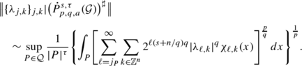
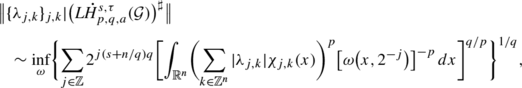
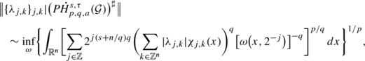
For all admissible parameters (in particular for a≫1), let $\dot{f}^{s,\tau}_{p,q} := (\dot{P}^{s+n/2-n/q,\tau}_{p,q,a}({\mathcal{G}}))^{\sharp}$, $\dot{b}^{s,\tau}_{p,q} := (\dot{L}^{s+n/2-n/q,\tau}_{p,q,a}({\mathcal{G}}))^{\sharp}$, $b\dot{h}^{s,\tau}_{p,q} := (L\!\dot{H}^{s+n/2-n/q,\tau}_{p,q,a}({\mathcal{G}}))^{\sharp}$ and $f\dot{h}^{s,\tau}_{p,q} := (P\!\dot{H}^{s+n/2-n/q,\tau}_{p,q,a}({\mathcal{G}}))^{\sharp}$.

6 Wavelet Characterizations

In this section, as an application of the coorbit interpretations in Theorems 5.11 and 5.12, we obtain wavelet characterizations for the spaces $\dot{B}^{s,\tau}_{p,q}({\mathbb{R}}^{n})$, $\dot{F}^{s,\tau}_{p,q}({\mathbb{R}}^{n})$, $B\!\dot{H}^{s,\tau}_{p,q}({\mathbb{R}}^{n})$ and $F\!\dot{H}^{s,\tau}_{p,q}({\mathbb{R}}^{n})$ for the full range of parameters extending the results in [62, Sect. 8.2] where mainly positive smoothness is considered. We use biorthogonal wavelet bases on ℝⁿ (see, for example, [7, 12]), namely, a system

(6.1)

with k,ℓ,m,j∈ℤ, of scaling functions $(\psi^{0}, \widetilde{\psi}^{0})$ and associated wavelets $(\psi^{1},\widetilde{\psi}^{1})$, where δ _k,ℓ =1 if k=ℓ else δ _k,ℓ =0 and δ _{(j,k),(ℓ,m)}=1 if j=ℓ and k=m else δ _k,ℓ =0. Notice that the latter includes that, for every f∈L ²(ℝ),

holds in L ²(ℝ). We now construct a basis in L ²(ℝⁿ) by using the well-known tensor product procedure. Consider the tensor products $\varPsi^{c} = \bigotimes_{j=1}^{n} \psi^{c_{j}}$ and $\widetilde{\varPsi}^{c} = \bigotimes_{j=1}^{n} \widetilde{\psi}^{c_{j}}$, c∈E:={0,1}ⁿ∖{(0,…,0)}. The following result is well known for orthonormal wavelets (see, for instance, [53, Sect. 5.1]), however straightforward to prove for biorthogonal wavelets.

Lemma 6.1

For any given biorthogonal system (6.1) and all f∈L ²(ℝⁿ),

(6.2)

with convergence in L ²(ℝⁿ).

Our aim is to specify, namely, state precise sufficient conditions on ψ ⁰, ψ ¹, $\widetilde{\psi}^{1}$ and $\widetilde{\psi}^{0}$ such that the representation (6.2) extends to the spaces considered above. Our method is to apply the abstract Theorem 4.7 to this specific situation. As the first step we check under which conditions the functions Ψ ^c and $\widetilde{\varPsi}^{c}$ belong to the set B(Y), where Y represents a Peetre-type space from Sect. 5.1.

Proposition 6.2

Let L∈ℕ, K∈(0,∞), and ψ ⁰,ψ ¹∈L ²(ℝ), where ψ ⁰ satisfies (D) and (S _K ), and ψ ¹ satisfies (D), (S _K ) and (M _L−1). Let ${\mathcal{G}}$ be an ax+b-group and $V :=[-1,1]^{n} \times (1/2,1] \subset \mathcal{G}$ a neighborhood of the identity $e\in \mathcal{G}$. Suppose further that for r ₁,r ₂∈ℝ, the weight w is given by $w(x,t) :=(1+|x|)^{v}(t^{r_{2}}+t^{-r_{1}})$ for all $(x,t) \in \mathcal{G}$. If p∈(0,1] and

(6.3)

then for all c∈E,

(6.4)

Proof

By the assumptions on the wavelet system and c≠0, we see that Ψ ^c satisfies (D), (S _K ) and (M _L−1). Lemma 5.9 implies that, for all N∈ℕ, x∈ℝⁿ and t∈(0,∞),

and hence

Splitting the integral (6.4) into $\int_{0}^{1} \int_{{\mathbb{R}}^{n}} + \int_{1}^{\infty} \int_{{\mathbb{R}}^{n}}$ leads to the sufficient conditions (6.3) to ensure their finiteness, which completes the proof of Proposition 6.2. □

In what follows, we need the quantity

(6.5)

From now on, $(\psi^{0},\widetilde{\psi}^{0})$ and $(\psi^{1}, \widetilde{\psi}^{1})$ always denote a biorthogonal wavelet system satisfying (6.1). Our main results read as follows.

Theorem 6.3

Let s∈ℝ, τ∈[0,∞) and q∈(0,∞].

• (i) Let p∈(0,∞), ψ ⁰ and $\widetilde{\psi}^{0}$ satisfy (D) and (S _K ), and ψ ¹ and $\widetilde{\psi}^{1}$ satisfy (D), (S _K ) and (M _L−1), where (L∧K)>M(s,τ,p,q,1∧p∧q,n/(p∧q)) in view of (6.5), then every $f \in \dot{F}^{s,\tau}_{p,q}({\mathbb{R}}^{n})$ admits the decomposition (6.2), where the sequence

  

  (6.6)

  belongs to the sequence space $\dot{f}^{s,\tau}_{p,q}$ with equivalent (quasi-)norms.

  Conversely, an element $f\in (\mathcal{H}^{1}_{w_{Y}})^{\sim}$, where $Y :=\dot{P}^{s+n/2-n/q,\tau}_{p,q,a}({\mathcal{G}})$, belongs to $\dot{F}^{s,\tau}_{p,q}({\mathbb{R}}^{n})$ if the sequence (6.6) belongs to $\dot{f}^{s,\tau}_{p,q}$ with equivalent (quasi-)norms.

• (ii) If p∈(0,∞], ψ ⁰ and $\widetilde{\psi}^{0}$ satisfy (D) and (S _K ), and ψ ¹ and $\widetilde{\psi}^{1}$ satisfy (D), (S _K ) and (M _L−1), where (L∧K)>M(s,τ,p,q,1∧p∧q,n/p) in view of (6.5), then every $f \in \dot{B}^{s,\tau}_{p,q}({\mathbb{R}}^{n})$ admits the decomposition (6.2), where the sequence (6.6) belongs to the sequence space $\dot{b}^{s,\tau}_{p,q}$ with equivalent (quasi-)norms.

  Conversely, an element $f\in (\mathcal{H}^{1}_{w_{Y}})^{\sim}$, where $Y :=\dot{L}^{s+n/2-n/q,\tau}_{p,q,a}({\mathcal{G}})$, belongs to $\dot{B}^{s,\tau}_{p,q}({\mathbb{R}}^{n})$ if the sequence (6.6) belongs to $\dot{b}^{s,\tau}_{p,q}$ with equivalent (quasi-)norms.

Theorem 6.4

Let s∈ℝ, p∈(1,∞), q∈[1,∞), and τ∈[0,1/(p∨q)′].

• (i) Let ψ ⁰ and $\widetilde{\psi}^{0}$ satisfy (D) and (S _K ), and ψ ¹ and $\widetilde{\psi}^{1}$ satisfy (D), (S _K ) and (M _L−1), where (L∧K)>M(s,τ,p,q,1/((p∨q)′+1),n(1/p+τ)) in view of (6.5). Then every $f \in B\!\dot{H}^{s,\tau}_{p,q}({\mathbb{R}}^{n})$ admits the decomposition (6.2), where the sequence (6.6) belongs to the sequence space $b\dot{h}^{s,\tau}_{p,q}$ with equivalent (quasi-)norms.

  Conversely, an element $f\!\in\! (\mathcal{H}^{1}_{w_{Y}})^{\sim}$, where $Y\!:=\!L\!\dot{H}^{s+n/2-n/q,\tau}_{p,q,a}({\mathcal{G}})$, belongs to $B\!\dot{H}^{s,\tau}_{p,q}({\mathbb{R}}^{n})$ if the sequence (6.6) belongs to $b\dot{h}^{s,\tau}_{p,q}$ with equivalent (quasi-)norms.

• (ii) Let q∈(1,∞), ψ ⁰ and $\widetilde{\psi}^{0}$ satisfy (D) and (S _K ), and ψ ¹ and $\widetilde{\psi}^{1}$ satisfy (D), (S _K ) and (M _L−1), where (L∧K)>M(s,τ,p,q,1/((p∨q)′+1),n(1/(p∧q)+τ)) in view of (6.5). Then every $f \in F\!\dot{H}^{s,\tau}_{p,q}({\mathbb{R}}^{n})$ admits the decomposition (6.2), where the sequence (6.6) belongs to the sequence space $f\dot{h}^{s,\tau}_{p,q}$ with equivalent (quasi-)norms.

  Conversely, an element $f\!\in\!(\mathcal{H}^{1}_{w_{Y}})^{\sim}$, where $Y\!:=\!P\!\dot{H}^{s+n/2-n/q,\tau}_{p,q,a}({\mathcal{G}})$, belongs to $F\!\dot{H}^{s,\tau}_{p,q}({\mathbb{R}}^{n})$ if the sequence (6.6) belongs to $f\dot{h}^{s,\tau}_{p,q}$ with equivalent (quasi-)norms.

Proof

We prove both theorems simultaneously and start with the interpretations as coorbits in Theorems 5.11 and 5.12. Using Propositions 5.2 and 5.7, together with (4.3), we conclude that, when Y is one of the spaces $\dot{P}^{s+n/2-n/q,\tau}_{p,q,a}({\mathcal{G}}), \dot{L}^{s+n/2-n/q,\tau}_{p,q,a}({\mathcal{G}}),\ L\!\dot{H}^{s+n/2-n/q,\tau}_{p,q,a}({\mathcal{G}})$ and $P\!\dot{H}^{s+n/2-n/q,\tau}_{p,q,a}({\mathcal{G}})$, the relation $w_{Y}(x,t) \le (1+|x|)^{v}(t^{r_{2}}+t^{-r_{1}})$ holds true for all x∈ℝⁿ and t∈(0,∞), where

and v=a. We then use the abstract result in Theorem 4.7, together with (6.2), (4.4) and Proposition 6.2. Notice that the Aoki-Rolewicz-exponent p ^∗=1/((p∨q)′+1) in Theorem 6.4 and p ^∗=(1∧p∧q) in Theorem 6.3, which is needed in (4.4) and Proposition 6.2, is given in Remark 3.11(ii) and Remark 5.4(ii). Taking in addition the conditions on a∈(0,∞) in Theorems 5.11 and 5.12 into account, we conclude the proofs of Theorems 6.3 and 6.4. □

Remark 6.5

The wavelet decomposition characterization in terms of the Carleson measures for  BMO(ℝⁿ) is already obtained (see [31, p. 154, Theorem 4]), namely,  BMO(ℝⁿ) is characterized by wavelets in terms of the space $\dot{f}_{p,2}^{0,1/p}({{ {\mathbb{R}}}^{n}})$. The conditions on the wavelets used therein are much weaker than ours; see Theorem 6.3(i). Indeed, using the equivalence $\mathop{\mathrm{BMO}}({\mathbb{R}}^{n}) = F^{0,1/p}_{p,2}({\mathbb{R}^{n}})$, where p is close to infinity, we obtain the condition K,L∈(n,∞) in Theorem 6.3. Thus, we need more smoothness and vanishing moments for the wavelets. However, for spaces on the real line (namely, n=1), the condition is close to the optimal one in [31].

Remark 6.6

Comparing with the orthogonal wavelet characterizations of ${\dot {B}_{p,q}^{s,\tau }({{{\mathbb{R}}}^{n}})}$ and ${\dot {F}_{p,q}^{s,\tau }({{{\mathbb{R}}}^{n}})}$ obtained in [62, Theorem 8.2], therein the parameter s restricts to s∈(0,∞), we establish the biorthogonal wavelet characterizations of these spaces for all s∈ℝ in Theorem 6.3. The wavelet characterizations for Besov-Hausdorff spaces ${B\!\dot {H}_{p,q}^{s,\tau }({{{\mathbb{R}}}^{n}})}$ and Triebel-Lizorkin-Hausdorff spaces ${F\!\dot {H}_{p,q}^{s,\tau }({{{\mathbb{R}}}^{n}})}$ in Theorem 6.4 are totally new even for some special cases such as Hardy-Hausdorff spaces.

Remark 6.7

Notice that we use more general biorthogonal wavelet bases instead of classical orthogonal wavelet bases as it is done for instance in [50, Chap. 3], in case of inhomogeneous classical Besov and Triebel-Lizorkin spaces, and also in [8, 9, 23, 26–28, 35]. We refer to [14] for the spaces Q _α (ℝⁿ), and to [40] for the Triebel-Lizorkin-Morrey spaces. For some earlier results with biorthogonal wavelets on classical Besov-Triebel-Lizorkin spaces, we refer to [30]. Notice also that the conditions on K and L in Theorems 6.3 and 6.4 are not optimal. However, they represent precise sufficient conditions.

We conclude the paper with the following corollary, which characterizes the set of parameters, when the used wavelet system represents an unconditional basis. Notice that by the abstract Theorem 4.7, we always have the unconditional convergence of (6.2) in the weak ∗-topology induced by $(\mathcal{H}^{1}_{w_{Y}})^{\sim}$. Since the coefficients in the expansion (6.2) are always unique due to the biorthogonality relations (6.1), this can be seen as a sort of the weak unconditional basis. For an unconditional basis (in the strong sense) we further need the unconditional convergence of (6.2) in the (quasi-)norm of the respective space.

Corollary 6.8

Under the assumptions of Theorems 6.3 and 6.4, the used wavelet systems represent an unconditional basis in the respective spaces if and only if τ=0 and p,q∈(0,∞).

Proof

When τ=0 and p,q∈(0,∞), this follows from the fact that the finite sequences form a dense subspace in the respective sequence space. Let us disprove the unconditional basis property for the space $\dot{F}^{s,\tau}_{p,q}(\mathbb{R}^{n})$. For the other cases, the proof is similar. If τ∈(0,∞), we use the distribution

(6.7)

for some c∈E. Indeed, the right-hand side converges unconditionally in the topology of $(\mathcal{H}^{1}_{w_{Y}})^{\sim}$, where $Y :=\dot{P}^{s+n/2-n/q,\tau}_{p,q,a}({\mathcal{G}})$, and defines an element from the reservoir space $(\mathcal{H}^{1}_{w_{Y}})^{\sim}$. By the biorthogonality relations (6.1), together with Proposition 5.14 and Definition 5.18, we see that the sequence (6.6) belongs to the respective sequence space $\dot{f}^{s,\tau}_{p,q}({{ {\mathbb{R}}}^{n}})$. Indeed, since τ∈(0,∞), we have

Hence, by Theorem 6.3, f belongs to the space $\dot{F}^{s,\tau}_{p,q}(\mathbb{R}^{n})$ and (6.7) is its biorthogonal wavelet expansion. By using the equivalent sequence space (quasi-)norm in Proposition 5.14(ii), we see, by a similar computation, that (6.7) does not converge in the (quasi-)norm of $\dot{F}^{s,\tau}_{p,q}(\mathbb{R}^{n})$, which completes the proof of Corollary 6.8. □

References

Adams, D.R.: A note on Choquet integrals with respect to Hausdorff capacity. In: Function Spaces and Applications, Lund, 1986. Lecture Notes in Math., vol. 1302, pp. 115–124. Springer, Berlin (1988)
Adams, D.R., Xiao, J.: Nonlinear potential analysis on Morrey spaces and their capacities. Indiana Univ. Math. J. 53, 1629–1663 (2004)
Adams, D.R., Xiao, J.: Morrey potentials and harmonic maps. Commun. Math. Phys. 308, 439–456 (2011)
Adams, D.R., Xiao, J.: Regularity of Morrey commutators. Trans. Am. Math. Soc. 364, 4801–4818 (2012)
Adams, D.R., Xiao, J.: Morrey spaces in harmonic analysis. Ark. Mat. (2011). doi:10.1007/s11512-010-0134-0
Aoki, T.: Locally bounded linear topological space. Proc. Imp. Acad. (Tokyo) 18, 588–594 (1942)
Bownik, M.: Anisotropic Hardy Spaces and Wavelets. Mem. Am. Math. Soc., vol. 164, no. 781 (2003). vi+122 pp.
Bownik, M.: Atomic and molecular decompositions of anisotropic Besov spaces. Math. Z. 250, 539–571 (2005)
Bownik, M., Ho, K.: Atomic and molecular decompositions of anisotropic Triebel-Lizorkin spaces. Trans. Am. Math. Soc. 358, 1469–1510 (2006)
Bui, H.-Q., Paluszyński, M., Taibleson, M.H.: A maximal function characterization of weighted Besov-Lipschitz and Triebel-Lizorkin spaces. Stud. Math. 119, 219–246 (1996)
Bui, H.-Q., Paluszyński, M., Taibleson, M.H.: Characterization of the Besov-Lipschitz and Triebel-Lizorkin spaces. The case q<1. J. Fourier Anal. Appl. 3, 837–846 (1997). Special Issue
Cohen, A., Daubechies, I., Feauveau, J.-C.: Biorthogonal bases of compactly supported wavelets. Commun. Pure Appl. Math. 45, 485–560 (1992)
Coifman, R.R., Meyer, Y., Stein, E.M.: Some new function spaces and their applications to harmonic analysis. J. Funct. Anal. 62, 304–335 (1985)
Cui, L., Yang, Q.: On generalized Morrey spaces. Sib. Math. J. 46, 133–141 (2005)
Dafni, G., Xiao, J.: Some new tent spaces and duality theorems for fractional Carleson measures and Q α (ℝn). J. Funct. Anal. 208, 377–422 (2004)
Dafni, G., Xiao, J.: The dyadic structure and atomic decomposition of Q spaces in several real variables. Tohoku Math. J. 57(2), 119–145 (2005)
Essén, M., Janson, S., Peng, L., Xiao, J.: Q spaces of several real variables. Indiana Univ. Math. J. 49, 575–615 (2000)
Fefferman, C., Stein, E.M.: Some maximal inequalities. Am. J. Math. 93, 107–115 (1971)
Feichtinger, H.G., Gröchenig, K.: A unified approach to atomic decompositions via integrable group representations. In: Function Spaces and Applications, Lund, 1986. Lecture Notes in Math., vol. 1302, pp. 52–73. Springer, Berlin (1988)
Feichtinger, H.G., Gröchenig, K.: Banach spaces related to integrable group representations and their atomic decompositions. I. J. Funct. Anal. 86, 307–340 (1989)
Feichtinger, H.G., Gröchenig, K.: Banach spaces related to integrable group representations and their atomic decompositions. II. Monatshefte Math. 108, 129–148 (1989)
Frazier, M., Jawerth, B.: A discrete transform and decompositions of distribution spaces. J. Funct. Anal. 93, 34–170 (1990)
Frazier, M., Jawerth, B., Weiss, G.: Littlewood-Paley Theory and the Study of Function Spaces. CBMS Regional Conference Series in Mathematics, vol. 79. American Mathematical Society, Providence (1991). Published for the Conference Board of the Mathematical Sciences, Washington, viii+132 pp.
Gröchenig, K.: Unconditional bases in translation and dilation invariant function spaces on ℝn. In: Constructive Theory of Functions, Varna, 1987, pp. 174–183. Publ. House Bulgar. Acad. Sci, Sofia (1988)
Gröchenig, K.: Describing functions: atomic decompositions versus frames. Monatshefte Math. 112, 1–42 (1991)
Haroske, D.D., Piotrowska, I.: Atomic decompositions of function spaces with Muckenhoupt weights, and some relation to fractal analysis. Math. Nachr. 281, 1476–1494 (2008)
Haroske, D.D., Tamási, E.: Wavelet frames for distributions in anisotropic Besov spaces. Georgian Math. J. 12, 637–658 (2005)
Haroske, D.D., Triebel, H.: Wavelet bases and entropy numbers in weighted function spaces. Math. Nachr. 278, 108–132 (2005)
John, F., Nirenberg, L.: On functions of bounded mean oscillation. Commun. Pure Appl. Math. 14, 415–426 (1961)
Kyriazis, G.: Decomposition systems for function spaces. Stud. Math. 157, 133–169 (2003)
Meyer, Y.: Wavelets and Operators. Cambridge University Press, Cambridge (1992). Translated from the 1990 French original by D.H. Salinger
Morrey, C.B.: On the solutions of quasi-linear elliptic partial differential equations. Trans. Am. Math. Soc. 43, 126–166 (1938)
Rauhut, H.: Time-frequency and wavelet analysis of functions with symmetry properties. PhD thesis, Technical University of Munich, Logos-Verlag (2004)
Rauhut, H.: Coorbit space theory for quasi-Banach spaces. Stud. Math. 180, 237–253 (2007). Preprint version. http://rauhut.ins.uni-bonn.de/RauhutCSQB.pdf
Rauhut, H., Ullrich, T.: Generalized coorbit space theory and inhomogeneous function spaces of Besov-Lizorkin-Triebel type. J. Funct. Anal. 260, 3299–3362 (2011)
Rolewicz, S.: On a certain class of linear metric spaces. Bull. Acad. Pol. Sci., Cl. Trois. 5, 471–473 (1957)
Rychkov, V.S.: On a theorem of Bui, Paluszyński and Taibleson. Proc. Steklov Inst. Math. 227, 280–292 (1999)
Rychkov, V.S.: On restrictions and extensions of the Besov and Triebel-Lizorkin spaces with respect to Lipschitz domains. J. Lond. Math. Soc. 60, 237–257 (1999)
Rychkov, V.S.: Littlewood-Paley theory and function spaces with \(A^{\mathrm{loc}}_{p}\) weights. Math. Nachr. 224, 145–180 (2001)
Sawano, Y.: Wavelet characterization of Besov-Morrey and Triebel-Lizorkin-Morrey spaces. Funct. Approx. Comment. Math. 38, 93–107 (2008)
Sawano, Y.: A note on Besov-Morrey spaces and Triebel-Lizorkin-Morrey spaces. Acta Math. Sin. Engl. Ser. 25, 1223–1242 (2009)
Sawano, Y., Tanaka, H.: Decompositions of Besov-Morrey spaces and Triebel-Lizorkin-Morrey spaces. Math. Z. 257, 871–905 (2007)
Sawano, Y., Yang, D., Yuan, W.: New applications of Besov-type and Triebel-Lizorkin-type spaces. J. Math. Anal. Appl. 363, 73–85 (2010)
Schäfer, M.: Generalized Coorbit Space Theory for Quasi-Banach Spaces, Diploma-Thesis, Hausdorff Center for Mathematics & Institute for Numerical Simulation, Bonn (2012). 129 pp.
Stein, E.M.: Harmonic Analysis: Real-Variable Methods, Orthogonality, and Oscillatory Integrals. Princeton University Press, Princeton (1993). xiv+695 pp.
Strömberg, J.-O., Torchinsky, A.: Weighted Hardy Spaces. Lecture Notes in Math., vol. 1381. Springer, Berlin (1989). vi+193 pp.
Triebel, H.: Theory of Function Spaces. Birkhäuser, Basel (1983)
Triebel, H.: Characterizations of Besov-Hardy-Sobolev spaces: a unified approach. J. Approx. Theory 52, 162–203 (1988)
Triebel, H.: Theory of Function Spaces II. Birkhäuser, Basel (1992)
Triebel, H.: Theory of Function Spaces III. Birkhäuser, Basel (2006)
Tang, L., Xu, J.: Some properties of Morrey type Besov-Triebel spaces. Math. Nachr. 278, 904–914 (2005)
Ullrich, T.: Continuous characterizations of Besov-Lizorkin-Triebel spaces and new interpretations as coorbits. J. Funct. Spaces Appl. (2012). doi:10.1155/2012/163213. Article ID 163213, 47 pp.
Wojtaszczyk, P.: A Mathematical Introduction to Wavelets. Cambridge University Press, Cambridge (1997). xii+261 pp.
Xiao, J.: Holomorphic Q Classes. Lecture Notes in Math., vol. 1767. Springer, Berlin (2001). viii+112 pp.
Xiao, J.: Geometric Q p Functions. Frontiers in Mathematics. Birkhäuser, Basel (2006). x+240 pp.
Yang, D., Yuan, W.: A note on dyadic Hausdorff capacities. Bull. Sci. Math. 132, 500–509 (2008)
Yang, D., Yuan, W.: A new class of function spaces connecting Triebel-Lizorkin spaces and Q spaces. J. Funct. Anal. 255, 2760–2809 (2008)
Yang, D., Yuan, W.: New Besov-type spaces and Triebel-Lizorkin-type spaces including Q spaces. Math. Z. 265, 451–480 (2010)
Yang, D., Yuan, W.: Characterizations of Besov-type and Triebel-Lizorkin-type spaces via maximal functions and local means. Nonlinear Anal. 73, 3805–3820 (2010)
Yang, D., Yuan, W.: Relations among Besov-type spaces, Triebel-Lizorkin-type spaces and generalized Carleson measure spaces. Appl. Anal. (2011). doi:10.1080/00036811.2011.629610
Yuan, W., Sawano, Y., Yang, D.: Decompositions of Besov-Hausdorff and Triebel-Lizorkin-Hausdorff spaces and their applications. J. Math. Anal. Appl. 369, 736–757 (2010)
Yuan, W., Sickel, W., Yang, D.: Morrey and Campanato Meet Besov, Lizorkin and Triebel. Lecture Notes in Math. 2005. Springer, Berlin (2010). xi+281 pp.
Acknowledgements
The authors would like to thank the anonymous referees and Professor Hans Georg Feichtinger for making several useful suggestions which helped to improve the paper and its readability.
Author information
Authors and Affiliations
Corresponding author
Additional information
Communicated by Hans G. Feichtinger.
This work is partially supported by the GCOE program of Kyoto University and 2010 Joint Research Project Between China Scholarship Council and German Academic Exchange Service (PPP) (Grant No. LiuJinOu [2010]6066). Yoshihiro Sawano is supported by Grant-in-Aid for Young Scientists (B) (Grant No. 21740104) of Japan Society for the Promotion of Science. Dachun Yang is supported by the National Natural Science Foundation (Grant No. 11171027) of China and Program for Changjiang Scholars and Innovative Research Team in University of China. Wen Yuan is supported by the National Natural Science Foundation (Grant No. 11101038) of China.
Rights and permissions
About this article
Cite this article
Liang, Y., Sawano, Y., Ullrich, T. et al. New Characterizations of Besov-Triebel-Lizorkin-Hausdorff Spaces Including Coorbits and Wavelets. J Fourier Anal Appl 18, 1067–1111 (2012). https://doi.org/10.1007/s00041-012-9234-5
Received:
Revised:
Published:
Issue Date:
DOI: https://doi.org/10.1007/s00041-012-9234-5
Keywords
- Besov-type space
- Triebel-Lizorkin-type space
- Besov-Hausdorff space
- Triebel-Lizorkin-Hausdorff space
- Tent space
- Local means
- Peetre maximal function