An adaptive modal pushover analysis procedure (VMPA-A) for buildings subjected to bi-directional ground motions

Abstract

A new modal pushover analysis procedure (VMPA-A) is developed and implemented in MATLAB code for three-dimensional buildings subjected to bidirectional ground motions. VMPA-A uses stepwise force patterns to represent changes in the dynamic characteristics because of the accumulated structural damages. The hybrid-spectrum concept is introduced to account for the bidirectional ground motion effects. Due to enactments of the equal displacement rule and the secant stiffness-based linearization process, nonlinear analysis is performed for specific displacement targets without stipulation of full modal capacity curves for each mode. Horizontal components of an earthquake record are considered simultaneously, and the consistency between the force and displacement vectors for each mode is provided. These are the main advantages of the proposed procedure against modal pushover analysis (MPA). An existing 21-story reinforced concrete building is analyzed to exemplify VMPA-A. The response parameters such as displacements, story drifts, internal forces, strains, etc. are discussed by comparing the results of VMPA-A with nonlinear time history analyses, which is accepted as the “exact solution”. Though consistent demand estimations are obtained for story drifts, displacements and deformations, some conservative results are obtained for story shears.

1 Introduction

Performance-based designs have been in high demand since the 1990s. The nonlinear static procedure (NSP) is a simple technique for the performance evaluation of structures subjected to earthquake excitation. In general, the regulations focus on conventional pushover analyses, which are applied to the structure by an invariant lateral force distribution corresponding to the fundamental mode shape. Although nonlinear time history analyses (NTHA) has been accepted as the most reliable method to calculate the building responses, NSPs considering higher mode contributions give reasonable results.

Multi-mode pushover analysis procedures taking into account the higher mode effects may be classified into the following two categories: single-run and multi-run procedures. Single-run pushover analysis procedures work with combined modal force or displacement contributions. The force-based adaptive pushover (FAP) analysis (Elnashai 2001; Antonio and Pinho 2004a), displacement-based adaptive pushover (DAP) analysis (Antonio and Pinho 2004b) and the story shear-based adaptive pushover (SSAP) method (Shakeri et al. 2010) are single-run-type pushover analysis methods. Mode-compatible force vectors are applied discretely to the building in the case of multi-run pushover analysis procedures. MPA (Chopra and Goel 2002), consecutive modal pushover (CMP) analysis (Poursha et al. 2009), adaptive modal combination (AMC) analysis (Kalkan and Kunnath 2006) and incremental response spectrum (IRSA) analysis (Aydinoglu 2003) are the main multi-run pushover analysis procedures.

The application of multi-mode NSPs to unsymmetrical plan-buildings has become prominent in recent years (Chopra and Goel 2004; Poursha et al. 2011; Shakeri et al. 2012; Perus and Fajfar 2005; Marusic and Fajfar 2005; Kreslin and Fajfar 2011, 2012; Fajfar et al. 2005; Meireles et al. 2006; Bhatt and Bento 2011, 2014). The problem requires 3D pushover analyses accounting for the torsional response of the building.

Contemporary tall-building design codes (LATBSDC 2008; SEAONC 2007; CTBUH 2008; PEER 2009) recommend 2D NTHA in the design of tall buildings. Most recently, 3D multi-mode pushover procedures are extended to predict the earthquake demands of buildings with bidirectional ground motion (Meireles et al. 2006; Reyes 2009; Reyes and Chopra 2011a, b; Poursha et al. 2014; Fujii 2011, 2014; Lin and Tsai 2007, 2008; Lin et al. 2012a, b; Bosco et al. 2012, 2013; Manoukas et al. 2012; Manoukas and Avramidis 2014).

As an earliest challenge, Meireles et al. (2006) utilized DAP procedure in the adaptive pushover method for a 3D asymmetric structure subjected to bi-directional excitation. Their approach is rather different from the variant of modal pushover analyses (VMPA) (Surmeli and Yuksel 2015) because of two main aspects: (1) DAP is a single-run, VMPA is a multi-run pushover procedures, (2) DAP works with displacement or drift increments, while VMPA employs target displacement demand for a predefined earthquake level. In the application of DAP, target displacement demands in bi-directions were determined as the averages of the results of time history analyzes.

One of the original procedures considering the influence of bidirectional ground motions is MPA (Reyes 2009; Reyes and Chopra 2011a, b), but it has two shortcomings. (1) Invariant load patterns compatible with nth-mode shape that correspond to linear-elastic eigenvalues are applied to the structure; although, the inelastic deformations alter the mode shapes and frequencies. It is not conceivable to simultaneously tune the displacements of three degrees-of-freedoms at the selected node when the invariant load patterns are used. Reyes and Chopra (Reyes 2009; Reyes and Chopra 2011a, b) choose the principal earthquake direction of a building as the target degrees-of-freedom to push, and the perpendicular direction is kept free. However, for the case of adaptive load patterns, two displacement demands are provided. (2) The planar components of ground motion are applied separately. For each direction, the demand parameters of interest are combined by the CQC combination rule. Next, the effects of two ground motion components are combined by the SRSS combination rule. Two applications of modal combination rules may cause erroneous results.

Manoukas et al. (2012, 2014) established an equivalent single degree of freedom system (E-SDOF) considering multidirectional seismic effects. By assuming the X- and Y-directional components of ground motion are proportional to each other ($\ddot{u}_{x} = \kappa {\kern 1pt} \ddot{u}_{y}$), this procedure requires only uniaxial pushover analyses in two separate directions, avoiding the application of a simplified directional modal combination rule. Nonetheless, the assumption of the selecting directional scale factor (SF) as $\kappa = 0.3$ and the proportionality of the two ground motion components must be further investigated.

Fujii (2011) developed an NSP to determine the earthquake demands of a multi-story asymmetric building subjected to bidirectional ground motion. Two independent and equivalent SDOF models based on the principal direction of each modal response were utilized. The contribution of each modal response is directly estimated based on the unidirectional response in the principal direction. Recently, this procedure was extended to horizontal bidirectional ground motion acting at an arbitrary angle of incidence (Fujii 2014).

Lin and Tsai (2008) developed three-degrees-of-freedom modal systems to evaluate the demands of two-way asymmetric buildings, which are represented by two modal translations and one modal rotation for two-directional ground motions. Additionally, Lin and Tsai (2012a, b) established inelastic response spectra constructed from the inelastic three-degrees-of-freedom modal systems.

In this paper, a formerly developed VMPA-A (adaptive version of modal pushover analysis) that was capable of accounting for the unidirectional component of earthquake records (Surmeli and Yuksel 2015) is extended to use for buildings subjected to bidirectional ground motion effects. The hybrid spectrum is defined to account for the bidirectional effects simultaneously. The demands are calculated in two translational and rotational directions by applying an equal displacement rule in the hybrid spectrum. Important benefits of the procedure are as follows:

• 1. By the application of secant stiffness-based linearization, the nonlinear analysis is delimited to the target displacement points for discrete modes deprived of the necessity to determine the full capacity curve. This feature is superior compared to MPA.

• 2. 3D pushover analyses are performed for each mode using mode-shape compatible force vectors by simultaneously considering the bidirectional ground motion effects. Although a unique modal combination procedure is necessary in VMPA-A, double applications of modal combination rules are required in MPA.

• 3. A rational approach is defined for bidirectional ground motions as an alternative for performing uniaxial pushover analysis (Manoukas et al. 2012, 2014) with directional scale factors.

• 4. VMPA-A provides target displacements of the selected node for the X, Y and θ directions, simultaneously. This is further superior to MPA.

The equal displacement rule has been accepted as a simplified tool to estimate the target displacement of long-period structures. MPA (Chopra and Goel 2002) and IRSA (Aydinoglu 2003) also use the rule in their simplified versions. PMPA (Reyes and Chopra 2011b), which is the simplified version of MPA, considers the linear elastic response contributions of higher modes. For each mode, the target displacement of the inelastic SDOF system is estimated by multiplying the displacement of the corresponding linear system by the inelastic deformation ratio of C_Rn. Aydinoglu (2003) states that in mid- to high-rise buildings, the effective initial periods of the first few modes are likely to be longer than the characteristic period of the elastic acceleration spectrum; therefore, those modes automatically qualify for the equal displacement rule.

VMPA-A also employs the equal displacement rule to estimate earthquake displacement demands. The foremost drawback of the procedure is limitations related to the applicability of the rule for some structural systems. The procedure could be implicated for far-fault type records and perhaps some near-fault records, which do not include the impulsive forward directivity effects. Furthermore, dominant natural periods of the building should be greater than the corner period.

A MATLAB-based computer program called DOC3D_v2 (Surmeli and Yuksel 2012, 2015; Surmeli 2016), has been developed to apply VMPA-A in the analyses of 3D frame and/or shear-wall type structural systems.

This paper introduces VMPA-A for bidirectional ground motion effect and assesses its achievement in contradicting the “exact solution,” which refers to NTHA performed by Perform3D (2012) for an existing 21-story RC building.

2 VMPA-A for Three dimensional buildings subjected to bidirectional ground motions

2.1 Equation of motion

The equation of motion of a building subjected to two components of horizontal ground motion is formed in terms of stepwise dynamic characteristics due to the progressive yielding of structural members:

$${\mathbf{M}}\ddot{\mathbf{u}}(t) + {\mathbf{C}}^{(k)} {\dot{\mathbf{u}}}(t) + {\mathbf{K}}^{(k)} {\mathbf{u}}(t) = - {\mathbf{M}}\iota_{x} \,\ddot{u}_{gx} (t) - {\mathbf{M}}\iota_{y} \,\,\ddot{u}_{gy} (t)$$

(1)

where ${\mathbf{u}}(t)$ corresponds to a displacement vector relative to the ground, $\ddot{u}_{gx} (t)$ and $\ddot{u}_{gy} (t)$ are the acceleration components of the horizontal ground motion, $\iota_{x}$ and $\iota_{y}$ are influence vectors used to define the direction of the ground motion, and ${\mathbf{M}}$ represents the mass matrix and can be expressed by the following sub-matrices:

$${\mathbf{M}} = \left[ {\begin{array}{*{20}c} {\mathbf{m}} & 0 & 0 \\ 0 & {\mathbf{m}} & 0 \\ 0 & 0 & {{\mathbf{I}}_{0} } \\ \end{array} } \right] \, \iota_{x} = \left[ {\begin{array}{*{20}c} {\mathbf{1}} \\ 0 \\ 0 \\ \end{array} } \right] \, \iota_{y} = \left[ {\begin{array}{*{20}c} 0 \\ {\mathbf{1}} \\ 0 \\ \end{array} } \right]$$

(2)

where ${\mathbf{C}}^{{({\text{k}})}}$ and ${\mathbf{K}}^{{({\text{k}})}}$ are the stepwise damping and secant stiffness matrices, respectively. The superscript (k) corresponds to kth step of the analysis process.

2.2 Expansion of the equation of motion in modal coordinates

If the right-hand side of Eq. 1 is expanded as the summation of modal inertia force distributions, the following equation could be drawn:

$$- {\mathbf{M}}{\kern 1pt} \iota_{x} \,\ddot{u}_{gx} (t) - {\mathbf{M}}{\kern 1pt} \iota_{y} \,\ddot{u}_{gy} (t) = {\mathbf{S}}_{x} \,\ddot{u}_{gx} (t) + {\mathbf{S}}_{y} \,\ddot{u}_{gy} (t) = \sum\limits_{n = 1}^{N} {\left( {{\mathbf{s}}_{nx}^{(k)} \ddot{u}_{gx} (t) + {\mathbf{s}}_{ny}^{(k)} \ddot{u}_{gy} (t)} \right)}$$

(3)

$${\mathbf{s}}_{nx}^{(k)} = \left[ {\begin{array}{*{20}c} {{\mathbf{s}}_{xn,x}^{(k)} } \\ {{\mathbf{s}}_{yn,x}^{(k)} } \\ {{\mathbf{s}}_{\theta n,x}^{(k)} } \\ \end{array} } \right] =\Gamma _{nx}^{(k)} M\,\phi_{n}^{(k)} =\Gamma _{nx}^{(k)} \left[ {\begin{array}{*{20}c} {{\mathbf{m}}\,\phi_{xn}^{(k)} } \\ {{\mathbf{m}}\,\phi_{yn}^{(k)} } \\ {{\mathbf{I}}_{0} \,\phi_{\theta n}^{(k)} } \\ \end{array} } \right]\quad s_{ny}^{(k)} = \left[ {\begin{array}{*{20}c} {{\mathbf{s}}_{xn,y}^{(k)} } \\ {{\mathbf{s}}_{yn,y}^{(k)} } \\ {{\mathbf{s}}_{\theta n,y}^{(k)} } \\ \end{array} } \right] =\Gamma _{ny}^{(k)} M\,\phi_{n}^{(k)} =\Gamma _{ny}^{(k)} \left[ {\begin{array}{*{20}c} {{\mathbf{m}}\,\phi_{xn}^{(k)} } \\ {{\mathbf{m}}\,\phi_{yn}^{(k)} } \\ {{\mathbf{I}}_{0} \,\phi_{\theta n}^{(k)} } \\ \end{array} } \right]$$

(4)

where ${\mathbf{S}}_{x}$ and ${\mathbf{S}}_{y}$ are spatial distributions of the effective earthquake force vectors, ${\mathbf{s}}_{nx}$ and ${\mathbf{s}}_{ny}$ are the contributions of the nth mode, and $\Gamma _{nx}$ and $\Gamma_{ny}$ are modal participation factors for the nth mode. The mode shape vector ($\phi_{n}$) consists of the $\phi_{xn}$, $\phi_{yn}$ and $\phi_{\theta n}$ terms corresponding to X and Y translational and Z rotational components of the vector, respectively.

The equation of motion could be rearranged in terms of the modal coordinates. The expansion of the physical displacement to the modal coordinates is as follows:

$$u_{n} (t) = \phi_{n}^{(k)} q_{n} (t)$$

(5)

where $q_{n} (t)$ is the modal displacement for the nth mode. If rigid diaphragm assumption is considered, the nth mode displacement vector $u_{n} (t)$ can be divided into three sub-vectors having N terms. N stands for story number, $u_{xn}$ and $u_{yn}$ are sub-vectors for the translational displacements in the X and Y directions, and $u_{\theta n}$ is the sub-vector for the torsional displacement.

$$u_{n} = \left[ {\begin{array}{*{20}c} {u_{xn} } \\ {u_{yn} } \\ {u_{\theta n} } \\ \end{array} } \right]$$

(6)

If Eq. 1 is defined in terms of the modal coordinates, both sides of Eq. 1 are multiplied by $\phi_{n}^{(k)T}$ and the result is divided by $\phi_{n}^{(k)T} {\mathbf{M}}\,\phi_{n}^{(k)}$, Eq. 7 is achieved.

$$\ddot{q}_{n} (t) + 2\xi_{n}^{(k)} \omega_{n}^{\,(k)} \dot{q}_{n} (t) + \left( {\omega_{n}^{(k)} } \right)^{2} q_{n} (t) = -\Gamma _{nx}^{(k)} \ddot{u}_{gx} (t) -\Gamma _{ny}^{(k)} \ddot{u}_{gy} (t)$$

(7)

where $\xi_{n}^{{{\kern 1pt} (k)}}$ stands for the damping ratio of the system and $\omega_{n}^{{{\kern 1pt} (k)}}$ is the stepwise vibration frequency.

If one benefits from the solution of a single component of ground motion (SDOF), the displacement demands can be calculated from Eq. 8:

$$\ddot{d}_{nx} (t) + 2\xi_{n}^{(k)} \omega_{n}^{\,(k)} \dot{d}_{nx} (t) + \left( {\omega_{n}^{(k)} } \right)^{2} d_{nx} (t) = - \ddot{u}_{gx} (t)$$

(8a)

$$\ddot{d}_{ny} (t) + 2\xi_{n}^{(k)} \omega_{n}^{\,(k)} \dot{d}_{ny} (t) + \left( {\omega_{n}^{(k)} } \right)^{2} d_{ny} (t) = - \ddot{u}_{gy} (t)$$

(8b)

where $d_{nx}$ and $d_{ny}$ are displacement vectors corresponding to the two horizontal components of ground motion. In Eq. 8, the last terms on the left-hand side could be considered as the stepwise pseudo-acceleration response ($a_{nx}^{(k)} (t)$ and $a_{ny}^{(k)} (t)$) of the nth mode. If they are re-arranged, the modal response of each mode could be expressed as:

$$\ddot{d}_{nx} (t) + 2\xi_{n}^{(k)} \omega_{n}^{\,(k)} \dot{d}_{nx} (t) + a_{nx}^{(k)} (t) = - \ddot{u}_{gx} (t)$$

(9a)

$$\ddot{d}_{ny} (t) + 2\xi_{n}^{(k)} \omega_{n}^{\,(k)} \dot{d}_{ny} (t) + a_{ny}^{(k)} (t) = - \ddot{u}_{gy} (t)$$

(9b)

The solution of Eqs. 9a and 9b as SDOF systems yields the maximum modal displacement demands $D_{nx}$ and $D_{ny}$. Equation 10 could determine the corresponding modal coordinates for each mode:

$$q_{n} =\Gamma _{nx}^{(k)} D_{nx} +\Gamma _{ny}^{(k)} D_{ny}$$

(10)

Thus, the physical displacements can be expressed by Eq. 11:

$$u_{n} =\Gamma _{nx}^{(k)} \phi_{n}^{(k)} D_{nx} +\Gamma _{ny}^{(k)} \phi_{n}^{(k)} D_{ny}$$

(11)

2.3 Implementation of VMPA-A for bidirectional ground motions

The implementation of VMPA-A for bidirectional ground motions will be described by the representative building shown in Fig. 1. Herein, though symmetrical distribution of the lateral load-carrying elements in the plan is supplied, some extent of eccentricity exists because of the non-uniform mass distribution. This procedure is restricted to torsionally stiff buildings.

Fig. 1

A representative building

The successive application steps of the procedure are listed below:

• 1. The initial eigenvalue analysis is conducted. Mode shapes $(\phi_{n}^{(1)} )$, natural frequencies $(\omega_{n}^{(1)} )$, modal participation factors ($\Gamma _{n}$) and modal participation mass ratios $(M_{n} )$ are obtained. The superscript (¹) stands for the first iteration step, while (^k) is used for the successive steps. A linear static analysis is performed for gravity loads and the demand parameters of interest ($r_{g}$) are obtained. The modes are sorted from largest-to-smallest modal participation mass ratios in X, Y and torsional directions. The X- and Y- directional and torsional modes are grouped as triplets, and a sufficient number of mode triplets should be selected in order to predict the earthquake demands accurately.

  Hybrid spectrum which is based on the assumption of spectral accelerations (S_ax and S_ay) in two perpendicular directions arise simultaneously, is proposed here to combine the uni-directional effects. Hybrid spectrum is originated from ADRS approach. Modal coordinates were obtained by Eq. 10. Spectral displacement vector and spectral force vectors are calculated from Eqs. 12 and 13, respectively.

  $$u_{n} = \phi_{n}^{(k)} \left( {\Gamma _{nx}^{(k)} S_{dnx} +\Gamma _{ny}^{(k)} S_{dny} } \right)$$

  (12)
  $$Q_{0nx}^{(k)} = s_{nx}^{(k)} = {\text{M}}\;\phi_{xn}^{(k)} \left( {\Gamma _{nx}^{(k)} \,S_{an\_ex} +\Gamma _{ny}^{(k)} \,S_{an\_ey} } \right)$$
  $$Q_{0ny}^{(k)} = s_{ny}^{(k)} = {\text{M}}\;\phi_{yn}^{(k)} \left( {\Gamma _{nx}^{(k)} \,S_{an\_ex} +\Gamma _{ny}^{(k)} \,S_{an\_ey} } \right)$$

  (13)
  $$Q_{0n\theta }^{(k)} = s_{n\theta }^{(k)} = {\text{M }}\phi_{\theta n}^{(k)} \left( {\Gamma _{nx}^{(k)} \,S_{an\_ex} +\Gamma _{ny}^{(k)} \,S_{an\_ey} } \right)$$

  The terms in parenthesis of Eqs. 12 and 13 namely hybrid spectral displacement ($\Gamma _{nx} \,S_{dx} +\Gamma _{ny} \,S_{dy}$) and hybrid spectral acceleration ($\Gamma_{nx} \,S_{ax} + \Gamma_{ny} \,S_{ay}$) are abscissa and ordinate of the hybrid spectrum. Employment of the equal displacement rule to first triplet of the modes is demonstrated in Fig. 2. Since modal participation factors ($\Gamma _{nx}$, $\Gamma _{ny}$) are dissimilar for each mode, the equal displacement rule is applied for discrete hybrid spectrums generated for the specific modes, see different colors in Figs. 2 and 5.

  Fig. 2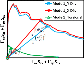

  

  Application of the equal displacement rule in the hybrid spectrum

  Hybrid spectral displacement and acceleration are accomplished by intersecting the line with a slope of $\left( {\omega_{n}^{(1)} } \right)_{{}}^{2}$ in the hybrid spectrum. $\left( {\omega_{x1}^{(1)} } \right)_{{}}^{2}$, $\left( {\omega_{y1}^{(1)} } \right)_{{}}^{2}$ and $\left( {\omega_{\theta 1}^{(1)} } \right)_{{}}^{2}$ are the initial eigenvalues of the first triplet.

• 2. The target physical displacement demands at node m are determined for each mode as follows:

  $$D_{mn\_x}^{(k)} = D_{mn\_gx} + \phi_{mn\_x}^{(k)} \left( {\Gamma _{nx}^{(k)} \,S_{dn\_x} +\Gamma _{ny}^{(k)} \,S_{dn\_y} } \right)$$

  (14)
  $$D_{mn\_y}^{(k)} = D_{mn\_gy} + \phi_{mn\_y}^{(k)} \left( {\Gamma _{nx}^{(k)} \,S_{dn\_x} +\Gamma _{ny}^{(k)} \,S_{dn\_y} } \right)$$

  (15)
  $$D_{mn\_\theta }^{(k)} = D_{mn\_g\theta } + \phi_{mn\_\theta }^{(k)} \left( {\Gamma _{nx}^{(k)} \,S_{dn\_x} +\Gamma _{ny}^{(k)} \,S_{dn\_y} } \right)$$

  (16)

  where $D_{mn\_gx}$, $D_{mn\_gy}$ and $D_{mn\_g\theta }$ are the X- and Y-translational and $\theta$-rotational displacement components of node m due to gravity loading, respectively. The target displacements of $D_{mn\_x}$, $D_{mn\_y}$ and $D_{mn\_\theta }$ are updated at each linearization step (k). The contributions of the first triplet of the modes to the total displacement demand in the representative building are shown schematically in Fig. 3.

• 3. The mode-compatible force vectors are obtained from the elastic spectral accelerations, Eq. 13. For each linearization step (k > 1), eigenvalue analysis is repeated and the stepwise mode-shape vector ($\phi_{n}^{(k)}$) is determined.

• 4. An algorithm is employed to calculate the inelastic hybrid spectrum ordinates corresponding to the target displacement and has three DOFs, namely $D_{mn\_x}$, $D_{mn\_y}$ and $D_{mn\_\theta }$ for each mode. The DOF with the maximum modal participation mass ratio is designated the reference in the pushover analysis. Displacement and force vectors are updated at each loading phase in VMPA-A. Therefore, three displacement demands are contemporarily provided. The equilibrium equation for the kth linearization step is written as follows:

  $${\mathbf{S}}_{n}^{(k)} {\mathbf{D}}_{n}^{(k)} + {\mathbf{P}}_{0n}^{(k)} = {\mathbf{Q}}_{n}^{(k)}$$

  (17)

  where ${\mathbf{S}}_{n}^{(k)}$, ${\mathbf{P}}_{0n}^{(k)}$ and ${\mathbf{Q}}_{n}^{(k)}$ are the stepwise stiffness matrix, the member load vector and the nodal load vector that provides target displacements at the reference DOFs for the nth mode, respectively. ${\mathbf{Q}}_{n}^{(k)}$ is defined in a scaled form depending on the stepwise force distribution vector ${\mathbf{Q}}_{0n}^{(k)}$ as follows:

  $${\mathbf{Q}}_{n}^{(k)} = \alpha_{n}^{(k)} \cdot {\mathbf{Q}}_{0n}^{(k)}$$

  (18)

  Fig. 3

  

  Contributions of the first triplet of the modes to the total displacement

  The loading parameter $\alpha_{n}^{(k)}$ represents the attainment ratio of the target displacement for a specific motion intensity.

• 5. A secant stiffness-based linearization procedure is implemented in the nonlinear analysis. The procedure is utilized not only for moment–curvature relations but also for strain–stress relations, (Fig. 4). At each iteration step, the effective rigidity of any section or fiber ($EI_{\;n}^{(k)}$, $E_{\;n}^{(k)}$) is determined from the constitutive relations.

  Fig. 4

  

  Linearization procedure

• 6. Succeeding the linearization (k > 1), an eigenvalue analysis is performed to determine the stepwise mode shapes ($\phi_{n}^{(k)}$) and natural frequencies ($\omega_{n}^{(k)}$).

• 7. Steps 4 to 7 are repeated until the parameter of $\alpha_{n}^{(k)}$ is acceptably close between two successive steps. Final $\alpha_{n}^{(p)}$ corresponds to the anticipated load parameter. The iteration step of k is exemplified on the hybrid spectrum in Fig. 5a. For the given example, the first X- and Y-translational modes behave nonlinearly and the first torsional mode is in the linear range. The last iteration steps of the first triplet of modes are presented in Fig. 5b.

  Fig. 5

  

  Hybrid spectrum format. a An intermediate step, b determination of loading parameter

  Equation 19 is utilized to determine the loading parameter. It represents the ratio of plastic to elastic base shears. The modal mass of nth mode for kth step $\left( {\phi_{n}^{(k)T} {\text{M}}\,\phi_{n}^{(k)} } \right)$ equals the unity in the mass normalized case, so the equation is rewritten in the short form.

  $$\begin{aligned} \alpha_{{n{\kern 1pt} }}^{(p)} = \frac{{\left( {\left( {\phi_{n}^{(p)T} \,{\mathbf{M}}{\kern 1pt} \,\iota } \right)^{2} /\left( {\phi_{n}^{(p)T} \,{\mathbf{M}}\,\,\phi_{n}^{(p)} } \right)} \right)\left( {\Gamma_{nx}^{(p)} \,S_{an\_px} + \Gamma_{ny}^{(p)} \,S_{an\_py} } \right)}}{{\left( {\left( {\phi_{n}^{(e)T} \,{\mathbf{M}}{\kern 1pt} \,\iota } \right)^{2} /\left( {\phi_{n}^{(e)T} \,{\mathbf{M}}\,\,\phi_{n}^{(e)} } \right)} \right)\left( {\Gamma_{nx}^{(e)} \,\,S_{an\_ex} + \Gamma_{ny}^{(e)} \,\,S_{an\_ey} } \right)}} \hfill \\ \alpha_{{n{\kern 1pt} }}^{(p)} = \frac{{\left( {\phi_{n}^{(p)T} \,{\mathbf{M}}{\kern 1pt} \,\iota } \right)^{2} \left( {\Gamma_{nx}^{(p)} \,S_{an\_px} + \Gamma_{ny}^{(p)} \,S_{an\_py} } \right)}}{{\left( {\phi_{n}^{(e)T} \,{\mathbf{M}}\,{\kern 1pt} \iota } \right)^{2} \left( {\Gamma_{nx}^{(e)} \,S_{an\_ex} + \Gamma_{ny}^{(e)} \,S_{an\_ey} } \right)}} \hfill \\ \end{aligned}$$

  (19)

  where the subscripts e and p stand for elastic and plastic cases, respectively.

• 8. Any demand parameter ($R_{n}$) of interest for the nth mode is obtained by Eq. 20.

  $$R_{n} = R_{n + g} - \,R_{g}$$

  (20)

  where $R_{n + g}$ and $R_{g}$ stand for the demands obtained from the pushover analysis with gravity loads and the sole gravity load analysis, respectively.

• 9. The resulting demand parameter $R$ is calculated using the combination rule of SRSS.

$$R = R_{g} { + }\sqrt {\left( {\sum\limits_{n = 1}^{N} {R{\kern 1pt}_{n}^{2} } } \right)}$$

(21)

3 Application of VMPA-A to an existing 21-story RC building

3.1 Modeling of the building

An existing 21-story RC building, which consists of three basements, one ground floor and 17 normal floors, is studied to assess the success of VMPA-A against the nonlinear time history analysis. The floor plans and elevations of the building are presented in Fig. 6. The total height of the building is 68.31 m. The story heights are 3.88, 2.75, 2.88, 3.55 and 3.25 m for the third, second and first basements, ground floor and typical floors, respectively.

Fig. 6

Floor plans and elevations of the existing 21 story RC building

The basements are surrounded with RC shear walls. The slabs between axes A-B1 and 1–6 are waffle type, while the other parts are flat slabs with 15 cm thickness. The typical cross sections of the structural members are shown in Fig. 7. The waffle slab is modeled by fictitious beam strip with 3.60 m in wide. The material qualities are examined from the destructive tests as follows: the concrete compressive strength is 27 MPa and the steel-yielding stress is 420 MPa. The firm type soil exists underneath the building, and the acceleration intensity of the design earthquake is defined as PGA = 0.4 g according to the Turkish Earthquake Code (TEC 2007).

Fig. 7

Cross sections and reinforcement details of the beams, the columns, and the shear walls

The gravity load analysis for slabs is shown in Table 1. The partitioning walls are represented by the additional distributed load with an intensity of 5 kN/m.

Table 1 Slab gravity loads

DOC3D_v2 (Surmeli and Yuksel 2012, 2015; Surmeli 2016) in which the VMPA-A procedure is implemented and Perform3D (CSI 2012) are utilized in the numerical analyses of the building. Fiber shell elements and 3D multiple vertical line elements (3D MVLEMs) (Vulcano et al. 1988; Fischinger et al. 2004; Kante 2005; Orakcal et al. 2006) are employed to represent shear walls in both of the programs.

In the model produced for Perform3D, the shear wall elements have no in-plane rotational stiffness at the nodes. To generate moment-resisting connections between a beam and a shear wall, an additional imbedded element is defined at the connection region. On the other hand, in the mathematical model produced for DOC3D_v2, rigid beams are involved at story levels to define the U-shaped geometry of the shear wall and make connections with the coupling beams.

Due to existing aspect ratio (height/length) and lateral reinforcement arrangements, shear deformations and shear-related failure modes of the shear walls are ignored by assigning high shear stiffness to the linear shear springs (k_Hx and k_Hy) in the 3D MVLEMs.

Plastic flexural hinges are defined at both ends of the beams. Moment curvature relations are idealized in the bilinear form, and the effective stiffness is defined as slope of the first line. Two programs for the calibration of curvatures accomplish preliminary first-mode pushover analyses. Rigid end offsets are defined for the beam to column connections in both programs.

Columns are modeled with fiber cross-section elements in Perform3D, whereas 3D MVLEMs are utilized in DOC3D. To provide double curvature on the columns because of horizontal loading, they are meshed into four elements.

The slabs are assumed to have infinite rigidity in their own-plane. Story masses defined in the translational directions are 344.1, 315.4, 338.4, 342.3 and 321.3 kNs²/m, while rotational masses are 13,571, 12,440, 13,345, 13,499 and 12,671 kNs²m for third, second and first basements, ground floor and typical floors, respectively.

Both programs accomplish modal analyses. In the analyses, the concrete modulus of elasticity of the shear walls and columns is taken as half of the initial value (0.5E₀) as suggested in ASCE/SEI 41.06 (2007). Very similar results are obtained from both programs, as presented in Table 2. Natural periods in the X and Y directions are 1.415 and 1.100 s, respectively.

Table 2 Natural periods and modal participation mass ratios of the building

To compare the response of the two models prepared in DOC3D_v2 and Perform3D, mode pushover analyses are performed in two orthogonal directions. The capacity curves obtained from two programs are consistent with each other, Fig. 8. The lateral load capacity in the Y direction is considerably larger than in the X direction, as expected. The critical Rayleigh damping ratio of 5%, with characteristic elastic periods of 0.2T₁ and 1.5T₁, is utilized in the nonlinear time history analyses achieved in Perform3D.

Fig. 8

Pushover curves obtained in X and Y directions

3.2 Ground motions selection

Thirty ground motions with two horizontal components, which are selected from 12 historical earthquakes, are utilized in the analyses. The records are selected from the PEER NGA database (2006). Important features of the earthquakes are listed in Table 3. A scaling procedure is applied to the records to match the mean spectral accelerations of the ground motions within the selected period range (0.2–2.0 s) to the specific Turkish Earthquake Code (TEC 2007) design spectrum.

Table 3 Selected historical earthquakes

The design spectrum is defined with two characteristic periods (T_a, T_b) related with soil type, effective ground acceleration factor (A₀ = 0.40) and building importance factor (I = 1.0). The characteristic periods are taken as T_a = 0.15 s, T_b = 0.40 s for firm soil (Z2). The X and Y components of the acceleration spectra, their mean spectrums and the target design spectrum are illustrated in Fig. 9.

Fig. 9

Spectrum curves of selected earthquake records

Depending on the results of the preliminary nonlinear time history analyses performed for the design earthquake, the structure does not experience nonlinearity because of its existing overdesigned capacity. Therefore, it is decided to scale-up the set of records by a scale factor of 2.5.

3.3 Comparisons for VMPA-A and NTHA

The verification of VMPA-A procedure implemented in DOC3D_v2 is executed by comparing its results with those obtained from NTHAs performed by Perform3D.

The 30 scaled historical earthquakes, which have two components, are imposed onto the X and Y axes of the building. The demand parameters considered are story displacements, drifts, shear forces, overturning moments, maximum compression-tension strains at some shear wall fibers and the distribution of the beam curvatures.

Three modal triplets, consisting of X, Y and θ_z displacement components, are utilized in the analyses. The triplets are selected by considering the modal mass participation. The ordinates of the hybrid spectrum are determined using the average spectrums of the X and Y components of the ground motions. Top displacement demands for each mode are given in Table 4 based on the hybrid spectrum (S_dxΓ_x + S_dyΓ_y).

Table 4 Displacement demands of the existing 21-story building

The implementation of the 3D VMPA-A procedure to the building is depicted in Fig. 10. The hybrid spectrum curves are given independently for the X, Y and θ_z modes. Application of the equal displacement rule to the first three modes is revealed with hollow markers on the spectrums. After the linearization process in VMPA-A, the elastic hybrid spectrum ordinates shown by hollow markers reduce to the plastic hybrid spectrum ordinates that are shown by filled markers. It is apparent that the first two translational (X and Y) modes are within the nonlinear range, whereas all of the torsional modes behave linearly.

Fig. 10

Implementation of 3D VMPA-A

All the response parameters are displayed in the same graphical format. The solid and dashed black lines correspond to the mean of the response parameter and the maximum-minimum values obtained from the NTHAs, respectively. The gray-painted area expresses the range between mean ± one standard deviation. The solid red, dashed blue and dashed green lines represent the results of VMPA-A, taking into account one, two and three modes, respectively.

The variation of the story displacements and drifts are shown in Fig. 11. The story displacements and drifts in both directions are generally well predicted. Although the deviation in the upper story is in the range of 5%, the discrepancy reaches to 30% for the lower story. The first mode governs the displacement profiles of the structure. The contribution of the higher modes is somewhat smaller.

Fig. 11

Comparisons of story displacements and drifts

The story shears and overturning moments are demonstrated in Fig. 12. The single mode analysis is not adequate to characterize the shear profiles. Comparable trends are also obtained for moments. Once two or three modes are considered, better estimations are obtained, especially for Y directional shear forces and the corresponding moments.

Fig. 12

Story shears and moments

Ultimate compression and tension strains obtained for Fibers 1, 2, 3 and 4 are depicted in Fig. 13. The strains attained for the ground floor, where the plasticity is mostly observed, are well predicted by single and multimode pushover analyses. A single mode pushover analysis is not successful to estimate the strains on the upper stories. Although tension strains are generally within the range of the mean ± one standard deviation band, the limits are exceeded for compression strains in the upper stories where an elastic response exists.

Fig. 13

Ultimate compression and tension strains

Curvature distributions for the selected beams are presented in Fig. 14. The single and multimode pushover analyses results are comparable. Multimode pushover results are permanently in the range of the mean ± one standard deviation band.

Fig. 14

Comparison of the curvatures for the selected beam sections

4 Conclusions

The following benefits of VMPA-A can be concluded.

• 1. The implementation of an equal displacement rule together with secant stiffness-based linearization in the hybrid spectrum format allows for a nonlinear analysis to be accomplished for the target displacement. It is not necessary to attain full modal capacity curves.

• 2. VMPA-A eliminates the stipulation of dual application of the modal combination rules.

• 3. Adaptive force patterns are applied to the structure at each step of the nonlinear analysis. Thus, displacement demands in three DOFs and the compatibility are provided concurrently.

The following conclusions can be drawn for the evaluated 21-story RC building:

• 1. The predictions obtained through the equal displacement rule for the displacements and drifts in both directions are in close agreement with the NTHA mean.

• 2. Conservative results are obtained for story shears and overturning moments, in general. First-mode behavior dominates story-overturning moments, especially for lower stories.

• 3. Ultimate tensile strains calculated for the selected shear wall fibers are comparable for VMPA-A and NTHAs. The compression strains are also consistent for the lower stories.

• 4. Beam curvatures are well estimated. First-mode governed the response.

• 5. The total execution time of VMPA-A is tremendously smaller than for NTHA.

For the case study considered, VMPA-A, obviously hybrid spectrum, exposed to be powerful tool and overall good quality results were obtained.

Further research is advised to determine the benefits and drawbacks of the hybrid spectrum especially for more irregular, complex and high-rise building structures.

References

Antonio S, Pinho R (2004a) Advantages and limitations of adaptive and non-adaptive force-based pushover procedures. J Earthq Eng 8(4):497–522
Antonio S, Pinho R (2004b) Development and verification of a displacement-based adaptive pushover procedure. J Earthq Eng 8(5):643–661
ASCE, SEI 41.06 (2007) Seismic rehabilitation of existing buildings, the latest generation of performance-based seismic rehabilitation methodology. ASCE, California
Aydinoğlu MN (2003) An incremental response spectrum analysis procedure based on inelastic spectral displacements for multi-mode seismic performance evaluation. Bull Earthq Eng 1:3–36
Bhatt C, Bento R (2011) Extension of CSM-FEMA440 to plan-asymmetric real building structures. Earthq Eng Struct Dynam 40(11):1263–1282
Bhatt C, Bento R (2014) The extended adaptive capacity spectrum method for the seismic assessment of plan-asymmetric buildings. Earthq Spectra 30(2):683–703
Bosco M, Ghersi A, Marino M (2012) Corrective eccentricities for assessment by the nonlinear static method of 3D structures subjected to bidirectional ground motions. Earthq Eng Struct Dynam 41:1751–1773
Bosco M, Ghersi A, Marino EM, Rossi PP (2013) Comparison of nonlinear static methods for the assessment of asymmetric buildings. Bull Earthq Eng 11:2287–2308
Chopra AK, Goel RK (2002) A modal pushover analysis procedure for estimating seismic demands for buildings. Earthq Eng Struct Dynam 31:561–582
Chopra AK, Goel RK (2004) A modal pushover analysis procedure to estimate seismic demands for unsymmetric-plan buildings. Earthq Eng Struct Dynam 33:903–927
CTBUH (2008) Recommendations for the seismic design of high-rise buildings. Council on Tall Buildings and Urban Habitat, Chicago
Elnashai AS (2001) Advanced inelastic static (pushover) analysis for earthquake applications. Struct Eng Mech 12(1):51–69
Fajfar P, Marusic D, Perus I (2005) Torsional effects in the pushover–based seismic analysis of buildings. J Earthq Eng 6:831–854
Fischinger M, Isakovic T, Kante P (2004) Implementation of a macro model to predict seismic response of RC structural walls. Comput Concr 1(2):211–226
Fujii K (2011) Nonlinear static procedure for multi-story asymmetric frame buildings considering bidirectional excitation. J Earthq Eng 15:245–273
Fujii K (2014) Prediction of the largest peak nonlinear seismic response of asymmetric buildings under bidirectional excitation using pushover analyses. Bull Earthq Eng 12:909–938
Kalkan E, Kunnath SK (2006) Adaptive modal combination procedure for nonlinear static analysis of building structures. J Struct Eng ASCE 132:1721–1731
Kante P (2005) Seismic vulnerability of reinforced concrete walls (in Slovenian). Ph.D. Dissertation, University of Ljubljana
Kreslin M, Fajfar P (2011) The extended N2 method taking into account higher mode effects in elevation. Earthq Eng Struct Dynam 40:1571–1589
Kreslin M, Fajfar P (2012) The extended N2 method considering higher mode effects in both plan and elevation. Bull Earthq Eng 10:695–715
LATBSDC (2008) An alternative procedure for seismic analysis and design of tall buildings located in the Los Angeles region. Los Angeles Tall Buildings Structural Design Council, Los Angeles, CA
Lin JL, Tsai KC (2007) Simplified seismic analysis of asymmetric building systems. Earthq Eng Struct Dynam 36:459–479
Lin JL, Tsai KC (2008) Seismic analysis of two-way asymmetric building systems under bidirectional seismic ground motions. Earthq Eng Struct Dyn 37:305–328
Lin JL, Tsai KC, Yang WC (2012a) Inelastic responses of two-way asymmetric-plan structures under bidirectional ground excitations-part I: modal parameters. Earthq Spectra 1:105–139
Lin JL, Yang WC, Tsai KC (2012b) Inelastic responses of two-way asymmetric-plan structures under bidirectional ground excitations-part II: response spectra. Earthq Spectra 1:141–157
Manoukas G, Avramidis I (2014) Evaluation of a multimode pushover procedure for asymmetric in plan buildings under biaxial seismic excitation. Bull Earthq Eng 12:2607–2632
Manoukas G, Athanatopoulou A, Avramidis I (2012) Multimode pushover analysis for asymmetric buildings under biaxial seismic excitation based on a new concept of the equivalent single degree of freedom system. Soil Dyn Earthq Eng 38:88–96
Marusic D, Fajfar P (2005) On the inelastic seismic response of asymmetric buildings under bi-axial excitation. Earthq Eng Struct Dynam 34:943–963
Meireles H, Pinho R, Bento R, Antoniou S (2006) Verification of an Adaptive Pushover Technique for the 3D Case. In: First European conference on earthquake engineering and seismology, Genewa
Orakcal K, Massone LM, Wallace JW (2006) Analytical modeling of reinforced concrete walls for predicting flexural and coupled-shear-flexural responses PEER Report 2006/7. Pacific Earthquake Engineering Research Center, University of California, Berkeley
PEER (2006) NGA Database Pacific Earthquake Engineering Research Center. University of California, Berkeley. http://peer.berkeley.edu/nga/
PEER (2009) Guidelines for seismic design of tall buildings. Pacific Earthquake Research Center, University of California, Berkeley
PERFORM3D V5.0. (2012) Nonlinear analysis and performance assessment of 3D structures. Computers and Structures Inc., Berkeley
Perus I, Fajfar P (2005) On the inelastic torsional response of single-storey structures under bi-axial excitation. Earthq Eng Struct Dynam 34:931–941
Poursha M, Khoshnoudian F, Moghadam AS (2009) A consecutive modal pushover procedure for estimating the seismic demands of tall buildings. Eng Struct 31:591–599
Poursha M, Khoshnoudian F, Moghadam AS (2011) A consecutive modal pushover procedure for nonlinear static analysis of one-way unsymmetric-plan tall building structures. Eng Struct 33:2417–2434
Poursha M, Khoshnoudian F, Moghadam AS (2014) The extended consecutive modal pushover procedure for estimating the seismic demands of two-way unsymmetric-plan tall buildings under influence of two horizontal components of ground motions. Soil Dyn Earthq Eng 63:162–173
Reyes JC (2009) Estimating seismic demands for performance-based engineering of buildings, Ph.D. dissertation. Department of Civil and Environmental Engineering, University of California, Berkeley
Reyes JC, Chopra AK (2011a) Three-dimensional modal pushover analysis of buildings subjected to two components of ground motion, including its evaluation for tall buildings. Earthq Eng Struct Dynam 40:789–806
Reyes JC, Chopra AK (2011b) Evaluation of three-dimensional modal pushover analysis for unsymmetric-plan buildings subjected to two components of ground motion. Earthq Eng Struct Dynam 40(13):1475–1494
SEAONC (2007) Recommended administrative bulletin on the seismic design and review of tall buildings using non-prescriptive procedures. Structural Engineers Association of Northern California, San Francisco
Shakeri K, Shayanfar MA, Kabeyasawa T (2010) A story shear-based adaptive pushover procedure for estimating seismic demands of buildings. Eng Struct 32:174–183
Shakeri K, Tarbali K, Mohebbi M (2012) An adaptive modal pushover procedure for asymmetric-plan buildings. Eng Struct 36:160–172
Surmeli M (2016) An adaptive modal pushover analysis procedure to evaluate the earthquake performance of high-rise buildings, Ph.D. dissertation. Graduate School of Science and Technology, Istanbul Technical University, Istanbul
Surmeli M, Yuksel E (2012) A flexibility based beam-column element capable of shear-flexure interaction. In: 15th World conference on earthquake engineering, Lisbon, Portugal
Surmeli M, Yuksel E (2015) A variant of modal pushover analyses (VMPA) based on a non-incremental procedure. Bull Earthq Eng 13(11):3353–3379
Turkish Earthquake Code (TEC) (2007) Ministry of public works and settlement Government of Turkey
Vulcano A, Bertero VV, Colotti V (1988) Analytical modelling of RC structural walls. In: Proceedings, 9th World conference on Earthquake
Author information
Authors and Affiliations
Corresponding author
Rights and permissions
About this article
Cite this article
Sürmeli, M., Yüksel, E. An adaptive modal pushover analysis procedure (VMPA-A) for buildings subjected to bi-directional ground motions. Bull Earthquake Eng 16, 5257–5277 (2018). https://doi.org/10.1007/s10518-018-0324-x
Received:
Accepted:
Published:
Issue Date:
DOI: https://doi.org/10.1007/s10518-018-0324-x