
Abstract
A variant of modal pushover analysis (VMPA) is presented to evaluate the seismic performance of the structures. The suggested procedure is based on an iterative process in which secant stiffnesses are used both at the element level and in the modal response. VMPA diverges from the existing modal pushover analyses for the following reasons: (1) mode compatible adaptive forces are applied to the structure at each iteration step, (2) the application of the equal displacement rule in combination with secant stiffness based linearization in the spectral displacement (Sd)—spectral acceleration (Sa) relation eliminates the necessity to produce a modal capacity diagram for each mode. The displacement controlled algorithm determines the single ordinate of the modal capacity diagram corresponding to the target displacement demand for the nth mode (Sdn_p, San_p) by reducing elastic spectral acceleration (San_e) to converge to the plastic acceleration (San_p). A Matlab based computer program known as DOC3D-v2 is developed to implement the proposed procedure. To verify the success of the suggested procedure, 9- and 20-storey LA SAC buildings are analysed, and the resulting demands are compared with several existing procedures, such as the extended N2, MPA and MMPA, as well as nonlinear time history analyses performed for two different set of acceleration records. VMPA yields enhanced results in terms of storey drifts, especially for the 20-storey LA building, compared with the other methods. Although the storey displacements and drifts are largely consistent with nonlinear time history analysis results, conservative estimates are obtained for the storey shear forces.
1 Introduction
Since the 1990s, the nonlinear static procedure (NSP) has become a practical analytical tool to estimate seismic demands of building type structures. Such regulations as ATC-40 (1996), FEMA 356 (2000), FEMA 440 (2005) and ASCE/SEI 41.06 (2007), mandate the implementation of NSP for the performance evaluation of structures. Most of NSPs are exactly designated as the conventional pushover analysis in which an invariant lateral force distribution corresponding to the fundamental mode shape is subjected to the structure. The target displacement demand is basically calculated using the smoothened design spectrum according to the capacity spectrum method (CSM, ATC-40) or the displacement coefficient method (FEMA 356). A type of capacity spectrum method, the N2 method, has been accepted as one of the most respected analysis methods by researchers (Fajfar and Fischinger 1988; Fajfar 1999, 2000). However, applicability of the conventional pushover analysis is limited to low-rise buildings without vertical or torsional irregularities (Krawinkler and Seneviratna 1998), the behaviour of which is not affected by higher modes. The first attempts to consider higher modes were made by Paret et al. (1996) and Sasaki et al. (1998). Subsequently, several multi-mode pushover analysis methods have been proposed. Modal pushover analysis (MPA) is one of the most frequently used procedures among researchers (Chopra and Goel 2002, 2004a, b; Chopra et al. 2004; Goel and Chopra 2005). In this method, the building is pushed with the lateral load patterns, which are appropriate with the discrete initial mode shapes, to a predetermined target displacement of a selected degree of freedom. The displacement demand for each mode is calculated through the inelastic response spectra or nonlinear time history analysis (NTHA), which is subjected to bi-linear single degree of freedom (SDOF) systems determined from the idealised capacity curves. An extension of the N2 method was proposed to account for higher modes in plan by Fajfar et al. (2005); more recently, the procedure was used to consider the higher mode effects in elevation by Kreslin et al. (2010, 2010a, 2011, 2012). The method offers a more simplified analysis tool with respect to MPA, which combines basic pushover analysis with the results of elastic modal analysis. Correction factors are introduced in the extended N2 method to scale the drift and displacement profiles in elevation and plan obtained from the single mode pushover analysis to provide the same drift and displacement profiles with the modal response spectrum analysis. Poursha et al. (2009) proposed a consecutive modal pushover procedure (CMP) for seismic assessment of tall buildings, in which the modal pushover analyses are implemented consecutively using lateral force patterns compatible with linear-elastic mode shapes. The procedure was applied to asymmetric tall buildings by Poursha et al. (2011). Khoshnoudian and Kashani (2012) introduced modified consecutive modal pushover analysis (MCMP), which is based on some modifications to CMP.
The above-mentioned multi-mode pushover procedures use invariant force distributions. Conversely, due to progressive yielding of the structural members, the dynamic characteristics of the structure undergo changes; as a result, the distribution of the lateral loads should be modified. To take into account the changes in dynamic characteristics, several adaptive pushover methods have been developed. The pioneer adaptive pushover application, which considers only single-mode behaviour, was proposed by Bracci et al. (1997). Following this study, multi-mode adaptive pushover procedures were proposed by many researchers, e.g., Elnashai (2001), Aydınoğlu (2003, 2004, 2007), Antonio and Pinho (2004a, 2004b), Kalkan and Kunnath (2006), Shakeri et al. (2010, 2012), and Abbasnia et al. (2013). The multi-mode adaptive methods may be classified into two groups. The first group is the single-run pushover analysis, in which the force or displacement distribution is calculated at each incremental step by combining mode contributions based on the instantaneous stiffness condition. The second group corresponds to multi-run pushover analysis, in which the building is subjected to mode compatible force vectors separately, and the contributions of demand parameter of interest are combined by an appropriate combination rule.
As a single-run pushover analysis type, force-based adaptive pushover analysis (FAP) was proposed by Elnashai (2001) and Antonio and Pinho (2004a). FAP suffers from the quadratic modal combination rules such as SRSS because the resulting forces are always positive at all storey levels. To overcome this problem, a modified version of FAP, namely, displacement-based adaptive pushover analysis (DAP), was developed by Antonio and Pinho (2004b), wherein the structure is subjected to displacements rather than forces. In this way, the sign reversal of forces at some storey levels is implicitly taken into account by structural equilibrium to provide the combined modal displacement profile. The DAP procedure was successfully applied in predicting the earthquake demands for structures in comparison with FAP (Antonio and Pinho 2004b). As a modified version of FAP, a storey shear-based adaptive pushover method known as SSAP was introduced by Shakeri et al. (2010) based on the storey shears that consider the reversal of sign in the higher modes, unlike the FAP method. The applied load vector at each step is calculated by subtracting the instantaneous combined modal shear forces of the consecutive stories. The implementation of the SSAP method to asymmetric-plan buildings was proposed by Shakeri et al. (2012). In this method, a lateral force in two translational directions and torques at each step are calculated by subtracting the combined modal storey shears and the combined modal storey torques of consecutive stories.
As a multi-run pushover analysis method, the adaptive modal combination (AMC) method proposed by Kalkan and Kunnath (2006) derives its fundamental shape from the adaptive pushover procedure of Gupta and Kunnath (2000). The AMC method combines the capacity spectrum method and the modal pushover procedure without the necessity for the pre-estimation of the target displacement. An energy-based methodology using constant-ductility inelastic displacement spectra is utilised to estimate the dynamic target point. A displacement-based adaptive procedure based on the effective modal mass combination rule (APAM) was proposed by Abbasnia et al. (2013) to address the sign reversals in the load vectors compatible with instantaneous mode shapes. The method uses the same methodology as CSM and AMC to estimate the target displacement. According to the modal mass combination rule, the load vector is scaled by a relative mode contribution factor that changes due to variations of dynamic characteristics. The combination of the modified load vectors is determined by summing/subtracting the modified load vectors. Each combination is applied to the structure independently, and the envelope of the results is utilised. However, for both the AMC and APAM methods, the interactions between the modes due to progressive yielding are not considered through the analysis process.
An incremental response spectrum analysis (IRSA) approach was proposed by Aydınoğlu (2003, 2004, 2007), in which a piece-wise linear incremental analysis procedure is conducted between formation of consecutive plastic hinges. As the backbone curves of modal hysteresis loops, modal capacity diagrams are used to estimate the modal inelastic displacement demands. The equal displacement rule with a smoothened elastic response spectrum was reported by Aydınoğlu (2003) as being a practical application of the method. The method uses a non-iterative pushover technique, and linear analysis is conducted using an instantaneous tangent stiffness matrix between formations of two consecutive plastic hinges. At each incremental pushover step, the structure is subjected to modal displacement or load patterns for the unit value of an unknown incremental scale factor. Analysis of the response spectrum is conducted to calculate the increment of the generic response quantity of interest. The resulting internal forces are then calculated by adding the increments to the previously obtained forces via the incremental scale factor. After the incremental scale factors of all potential plastic hinges are calculated, the smallest factor is selected as the indicator of development of the next plastic hinge. Once the incremental scale factors are obtained, the other demand parameters of interest are calculated accordingly.
The nonlinear structural analysis algorithms mostly use tangent stiffness, and require the determination of the capacity curve till a predetermined target displacement demand. The MPA method needs capacity curves in the form of modal displacement (Sd) versus modal pseudo-acceleration (Sa), (ADRS). Subsequently, modal displacement demands are calculated via NTHA using these curves. In the current study, a variant of modal pushover analysis (VMPA) is proposed as a new application of MPA. In VMPA, by the application of the equal displacement rule together with the secant stiffness based linearization technique, the nonlinear analysis is limited only to the target displacement points for individual modes without the necessity of the determination of full capacity curve that diverges from MPA. A displacement controlled algorithm is utilised to calculate the plastic modal capacity (Sap) corresponding to target displacement (Sdp) in the ADRS format, for a specific earthquake level.
The adaptive version of VMPA, which is called VMPA-A, considers the variation of dynamic characteristics due to progressive yielding of the structural members.
A MATLAB based computer program, the so-called DOC3D-v2, was developed to implement VMPA to analyse three-dimensional frame and/or shear-wall type structural systems. DOC3D-v2 takes into account concentrated and distributed plasticity for the frame type elements as well as considering the second-order effects of axial loads on the members. Furthermore, the beam-column element of DOC3D-v2 considers the nonlinear interaction of shear-flexural deformations, (Surmeli and Yuksel 2012). The applicability of the physical sub-structuring approach is one of the substantial features of DOC3D-v2 for reducing the computation time.
The main distinctions of VMPA from the existing procedures are presented as follows:
-
1.
One of the promising features of VMPA is to have the procedure applied for the determination of the plastic spectral acceleration (Sap). In this approach, the full modal capacity curve for each vibrational mode does not need to be obtained.
-
2.
The secant stiffness method is used in VMPA for the linearization of nonlinear constitutive models, which may have the horizontal and/or descending branches.
-
3.
Adaptive and non-adaptive versions of VMPA could be applied simply by the assignment of a key parameter. Application of the adaptive version is critical, especially for high-rise and irregular buildings.
The focal shortcoming of VMPA is the disregard of the modal interaction in the nonlinear range, as is the case for some other procedures.
The primary objective of this paper is to present VMPA and to discuss its rationality against NTHA, as well as the other principal procedures. The success of VMPA has been assessed against the increasing number of stories and the ground motion intensity.
2 A variant of modal pushover analysis (VMPA)
The theory behind the proposed algorithm is based on the solution of the equation of motion in terms of the modal coordinates and the application of an appropriate mode-superposition method to predict the demand parameter of interest. In this context, the essential information will be presented in the next chapters for VMPA-A, in which eigen-value analysis is repeated for each individual step of the nonlinear analysis. VMPA, which is a special case of VMPA-A, uses invariant vibrational mode shapes that depend on the initial stiffness of the structural members.
2.1 Equation of motion
The equation of motion for a building subjected to horizontal earthquake ground motion can be written in terms of the instantaneous dynamic characteristics due to progressive yielding of the structural members:
where \( {\mathbf{u}}(t) \) corresponds to the displacement vector relative to the ground, \( \textit{\"{u}}_{g} (t) \) is the horizontal ground motion acceleration, ι is the influence vector that is used for defining the direction of ground motion, \( {\mathbf{M}} \) represents the mass matrix, and \( {\mathbf{C}}^{{({\mathbf{k}})}} \) and \( {\mathbf{K}}^{{({\mathbf{k}})}} \) are the instantaneous damping and secant stiffness matrices, respectively.
2.2 Expansion of the equation of motion in modal coordinates
Although the solution of the equation of motion could be provided via step-by-step integration methods, mode-superposition method is a rational alternative. Aydınoğlu (2003) reported two important advantages of the mode-superposition method: (1) freedom in assigning the modal damping ratios in each mode and (2) superior accuracy obtained in the solution of the modal SDOF systems.
If right hand side of the equation of motion (Eq. 1) is expanded as the summation of modal inertia force distributions, then the following equation is obtained:
where \( {\mathbf{S}} \) is the spatial distribution of the effective earthquake force vectors, and \( {\mathbf{s}}_{n} \) is the contribution of the nth mode to the total, ϕ (k) n and \( \Gamma _{n}^{(k)} \) are the instantaneous mode shape vector and modal participation factor for the nth mode, respectively.
The equation of motion is rearranged in terms of the modal coordinates. The expansion of physical displacement to modal coordinates for the nth mode contribution is as follows:
q n (t) is the modal displacement for nth mode. If both sides of Eq. (1) are multiplied by ϕ (k)T n and divided by effective mass of nth mode \( \left( {M_{n} = \phi_{n}^{(k)T} \;{\mathbf{M}}\phi_{n}^{(k)} } \right), \) then the following is obtained:
where ξ (k) n denotes the damping ratio of the system, and ω (k) n is the instantaneous natural vibration frequency.
If one writes Eq. (4) for the SDOF system using d n (t) to denote the horizontal displacement, then the following equation is obtained:
Modal displacements could be defined in terms of the solution of the SDOF system,
Physical displacements could then be expressed as:
In Eq. (5), the last term on the left hand side could be considered as the instantaneous pseudo acceleration response (a (k) n (t)) of the nth mode. If Eq. (5) is re-arranged, then the modal response of each mode could be expressed as:
The incremental form of Eq. (8) was established by Aydınoğlu (2003), and solution of the equation was constructed in ADRS format, namely, modal hysteresis loops. The envelope of the modal hysteresis loops corresponds to the modal capacity diagram, which demonstrates the structure’s capacity for each mode in a demand dependent manner.
2.3 Equal displacement rule for calculating the earthquake demand
To calculate the displacement demand for the SDOF systems, the equal displacement rule is the simplest and most rational method to use compared to the capacity spectrum method, the displacement coefficient method, and NTHA. In the equal displacement rule, inelastic spectral displacement is assumed to be equal to elastic spectral displacement of SDOF system subjected to earthquake ground motion. However, some limitations exist on the applicability of the method. The method could only be implicated for far-fault earthquake records and perhaps some near-fault records, which do not include the impulsive forward directivity effects. Furthermore, the dominant natural period of the structure should be greater than the corner period. For the mid- to high-rise buildings, the higher modes having sufficient effective mass contributions to total response may have longer natural period than the corner period. Therefore, the use of equal displacement rule is reasonable to obtain the displacement demands for these modes as stated by Aydinoglu (2003).
2.4 The solution procedure
The developed algorithm is described on a representative example with 3 DOFs. The steps of the procedure are as follows:
-
1.
The initial eigenvalue analysis is conducted by using the gross stiffnesses of the structural members; based on the analysis, the mode shapes (ϕ (1) n ), natural frequencies (ω (1) n ) and modal participation factors (Γ (1) n ) are obtained. The superscript (1) denotes the definition of the first iteration step; the superscript will be defined as k for the succeeding statements. The nonlinear static analysis for gravity loads is performed, and the demand parameters of interest (R g ) is obtained.
-
2.
The equal displacement rule is applied in ADRS format, and the modal displacement demands for each mode are obtained, Fig. 1. The initial step of the procedure is to draw the smoothened design spectrum. The modal displacement demands (S dn_p ) and the consistent spectral accelerations (S an_e ) are attained from the intersection of the ADRS curve, with the lines having slopes of (ω (1) n )2. S dn_p is the target modal displacement demand, which does not change during analysis.
Fig. 1 
Application of the equal displacement rule in ADRS format
-
3.
Target physical displacement demand at the mth degree of freedom is determined for each mode using Eq. (9).
$$ D_{mn}^{(k)} = D_{mn\_g} + \phi_{mn}^{(k)} \cdot\Gamma _{n}^{(k)} \cdot S_{dn} $$(9)The target displacement of D (k) mn is instantly updated at each linearization step (k), as demonstrated in Fig. 2. In Eq. (9), D mn_g is the displacement demand due to gravity loading.
Fig. 2 
Target displacements for each mode at the kth linearization step
-
4.
The mode compatible force vectors obtained from elastic spectral accelerations are defined by Eq. (10).
$$ Q_{0n}^{(k)} = s_{n}^{(k)} =\Gamma _{n}^{(k)} \;{\mathbf{M}} \, \phi_{n}^{(k)} \;S_{an\_e} $$(10)The visual representations of spatial force distributions for the kth step are illustrated in Fig. 3. For the first step, spectral accelerations of \( S_{a1}^{(1)} ,\;S_{a2}^{(1)} \;{\text{and}}\;S_{a3}^{(1)} \) are taken as equal to the elastic spectrum ordinates of \( S_{a1\_e} ,\;S_{a2\_e} \;{\text{and}}\;S_{a3\_e} , \) Fig. 1.
Fig. 3 
The horizontal force patterns for modes at the kth step
-
5.
A displacement controlled algorithm is used to calculate the inelastic spectral accelerations conforming to the target displacements for each mode. The static equilibrium for the kth linearization step is given in Eq. (11).
$$ \varvec{S}_{n}^{(k)} \varvec{D}_{n}^{(k)} \; + \;\varvec{P}_{0n}^{(k)} = \varvec{Q}_{n}^{(k)} $$(11)where \( \varvec{S}_{n}^{(k)} ,\varvec{P}_{0n}^{(k)} \;\text{and}\;\varvec{Q}_{n}^{(k)} \) are the instantaneous static stiffness matrix, distributed loading vector and nodal load vector (which provides target displacement at the reference DOF for nth mode), respectively. The nodal load vector Q (k) n can be defined in a scaled form of the instantaneous force distribution vector for nth mode, Q (k)0n , as follows:
$$ \varvec{Q}_{n}^{(k)} = \alpha_{n}^{(k)} \cdot \varvec{Q}_{0n}^{(k)} $$(12) -
6.
The secant stiffness based linearization procedure is implemented in the analysis. The procedure is used not only for moment–curvature relations but also for strain–stress relationships for fibre elements, (Fig. 4). At each iteration step, effective rigidities of the any section or fibre (EI (k) n , E (k) n ) are attained from the constitutive relations.
Fig. 4 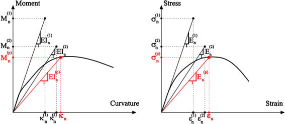
The linearization procedure
-
7.
After each linearization step (k > 1), eigenvalue analysis is repeated and the instantaneous mode shapes (ϕ (k) n ), natural frequencies (ω (k) n ) and modal participation factors (Γ (k) n ) are defined.
-
8.
The steps 3–7 are repeated until the parameter of α (k) n is sufficiently close between the successive steps. The final α (p) n corresponds to the desired load parameter. The kth iteration step is presented in Fig. 5a. For the given example, the first two modes behave nonlinearly, and the third one is in the linear range.
Fig. 5 
a An intermediate step in the ADRS spectrum. b The last iteration step in the ADRS spectrum
The last step in the iteration is presented in Fig. 5b. The resulting natural frequencies and plastic accelerations are presented as ω (p) n and San_p, respectively.
The loading parameters are defined by Eqs. (13) and (14) for the non-adaptive (VMPA) and adaptive (VMPA-A) cases, respectively.
$$ \alpha_{n}^{(p)} = \frac{{S_{an\_p} }}{{S_{an\_e} }} $$(13)$$ \alpha_{n}^{(p)} = \frac{{\left( {\phi_{n}^{(p)T} \;{\mathbf{M}}\iota } \right)^{2} S_{an\_p} }}{{\left( {\phi_{n}^{(1)T} \;{\mathbf{M}}\iota } \right)^{2} S_{an\_e} }} $$(14) -
9.
Any demand parameter (R n ) of interest for the nth mode, such as displacement, drift, internal force, curvature, fibre strains, etc., can be calculated as:
$$ R_{n} = R_{n + g} - R_{g} $$(15) -
10.
The processes of steps 3–9 are repeated for the desired number of modes (N).
-
11.
The SRSS modal combination rule is applied, and the resulting demand parameter of interest, R, is obtained as:
$$ R = R_{g} + \sqrt {\left( {R_{n}^{2} } \right)} $$(16) -
12.
The axial force-moment interaction is considered, not only for the discrete modal pushover analyses but also for the combination of axial loads on the columns. After the combined axial force (P) is calculated, the plastic moment (M p ) is determined from the interaction curve, Fig. 6a. The plastic moment is used to construct the moment–curvature relation. The combined moment (M) is calculated as a value corresponding to the combined curvature of κ PM , Fig. 6b.
Fig. 6 
Combined Internal Forces and Curvatures. a Axial force-moment interaction curve. b The moment corresponding to the combined curvature (κ PM )
-
13.
Once the combined moments are determined at the moment plastic hinges of the members, the corresponding shear forces are calculated by using the member equilibrium equations, Fig. 7 and Eq. (17).
$$ T_{i} = \frac{{M_{i} + M_{j} }}{L} + \frac{qL}{2}\quad \quad T_{j} = \frac{{M_{i} + M_{j} }}{L} - \frac{qL}{2} $$(17)Fig. 7 
End forces of a beam element
Detailed flow-chart of the algorithm is presented in Fig. 8.
Fig. 8 
Flow-chart of the proposed procedure


3 Benchmark structures and ground motion data
3.1 9- and 20-storey LA SAC steel frames
The test structures are 9- and 20-storey steel frame buildings, which were designed for the Los Angles (LA) region in the SAC Phase II project, Gupta and Krawinkler (1999). Kreslin and Fajfar (2011) also studied the buildings to demonstrate the validity of the extended N2 method against the results of response history analyses. The modelling assumptions and the selected earthquake record sets defined in the paper are taken as the basis for this paper. The results of VMPA and VMPA-A are compared with NTHA, MPA and the extended N2 method.
The buildings consist of two perimeter frames in each orthogonal direction as well as the gravity frames. For simplicity, instead of using 3D models of the lateral load-resisting part of the structure, only the perimeter frames in the north–south direction are modelled. The preferred model is designated as the M1 model by Gupta and Krawinkler (1999). In this model, the nonlinearities are taken into account with plastic hinges at the beam and column ends without rigid end offsets, and the behaviour of the panel zones are not considered. The elevations and sectional dimensions of the perimeter frames are presented in Fig. 9. The yield strengths of the columns and the beams are taken as 397 MPa and 339 MPa, respectively. The columns are pinned at the base. The column splices are arranged at 1.83 m above some of the storey levels.

SAC buildings (all dimensions in meters)
In the 9-storey building, the right end of the beams between the E and F axes are simply hinged. All other connections are fixed. The columns are arranged in the strongest direction, except the F axis. The ground level is restrained in the lateral direction to represent concrete foundation walls.
In the 20-storey building, all of the connections are fixed, except the bottom ends of the second basement columns. The beams are also simply connected to the columns at this level. The ground floor and first basement levels are laterally restrained against horizontal displacements. The columns of the A and F axes have tube sections. More details are found elsewhere, Gupta and Krawinkler (1999).
PERFORM-3D V5.0 (CSI 2011) software is used to model and analyse the test buildings. Bilinear elasto-plastic hinges are used at the member ends to represent the concentrated plasticity. The beams were modelled with simple moment hinges. PMM hinges are defined on the columns to represent the interaction between the axial force and the bending moments. Due to relatively low axial force intensities on the columns, second-order effects are neglected. The critical Rayleigh damping ratio of 5 % with characteristic elastic periods of the first and third modes are utilised in NTHA. The periods, modal participation factors and effective mass ratios are tabulated in Table 1 for the test buildings.
3.2 Ground motions
Two sets of ground motions are utilised in this study. Four intensities, namely, I 1, I 2, I 3 and I 4, are introduced based on the different ground acceleration levels (a g ) of 0.10, 0.50, 0.75, and 1.00×g, respectively.
The first set consists of 44 strong ground motion records, which are taken from the far fault set in FEMA-P695 project FEMA-P695 (2008). Originally, the records were downloaded from the PEER NGA Database (2006). The records were scaled so that the median spectral acceleration of the earthquake set coincides with the spectral acceleration value of the selected design spectrum at the first vibrational mode period of the benchmark buildings. The PEER NGA set is scaled only for the I 3 intensity.
The second set is taken from the European Database (Ambraseys et al. 2002) and consists of 20 strong ground motion records. The ground motions are simply scaled so that the spectral acceleration corresponding to the first mode period coincides with the spectral value of the design spectrum at the same period. The selected design spectrum is Eurocode 8 (EC8 2004) for soil type C.
The spectra drawn for the PEER NGA and the European Database for intensity level 3 (I 3) are presented in Fig. 10.

The scaled ground motion spectra: a 9-storey and b 20-storey building
4 Assessment of the VMPA
The assessment of the VMPA procedure is achieved by comparing the results of the procedure with those obtained from the NTHA. The evaluated demand parameters are storey displacements, drifts, shear forces and the distribution of column and beam curvatures.
The first step in the verification involves the 9-storey LA Building subjected to the El Centro record. Subsequently, the average of the NTHA results of two sets of ground motions are compared with the VMPA results for the benchmark structures. The differences between the results of the VMPA procedure and the results of the MPA, MMPA and extended N2 will be presented. The results obtained from the adaptive and non-adaptive versions of the VMPA are also assessed.
4.1 Evaluation for a specific earthquake
Two sets of analyses were performed using VMPA for 1.5 × El Centro ground motion. In the first set, the equal displacement rule is implemented to determine the displacement demand of the reference DOF for each mode. In the second set, the combined displacement demand in VMPA is made equivalent to the ultimate displacement demand obtained from NTHA at the reference DOF.
Chopra and Goel (2002) also studied the 9-storey LA Building with 1.5 × El Centro ground motion to validate the MPA procedure against the NTHA results. The NTHA analysis was performed without considering gravity loads, and a 2 % critical damping ratio was used, unlike the other NTHA results presented in the proceeding chapters. Considering the same structural and dynamic characteristics as Chopra and Goel (2002), the adaptive (VMPA-A) and non-adaptive (VMPA) procedures are conducted, and the resulting demands are compared. Figure 11 shows the results of the equal displacement rule, and Fig. 12 illustrates the results of the case in which the top storey displacement is tuned to the NTHA result.

Demands determined from the equal displacement rule for the 1.5 × El Centro Record

Demands determined from the imposed top displacement comes from the NTHA for the 1.5 × El Centro Record
From the application of the equal displacement rule procedure, a 26 % relative error is obtained at the top displacement compared with the NTHA results. The displacements at the lower stories are relatively similar in both cases. The MPA method provides better displacement demands for all stories in comparison with the VMPA procedure using the equal displacement rule.
Although the maximum relative errors for storey drifts obtained from the VMPA procedure using the equal displacement rule is higher than those of the MPA, in general, the estimation of VMPA provides better results, especially for the lower and upper stories. The predictions of the storey drifts in the second set are excellent between the third and seventh stories. For the remaining part, reasonable differences are observed.
The prediction of storey shears obtained from VMPA using the equal displacement rule is sufficient for all storeys. VMPA-A provides better results with respect to the non-adaptive analysis. Superior estimates for the storey shears are observed for the second set of analyses.
The curvatures at the bottom end of the columns positioned at the C axis are plotted in Figs. 11 and 12. The equal displacement rule produces good results; the second set yields better results, except for the fourth storey.
As another comparison, the curvatures of the outer beams are poorly predicted for both of the analyses sets. Chopra and Goel (2002) also represented plastic rotations of the outer beams determined from MPA. However, VMPA uses curvature type plastic hinges, and the total curvatures are considered.
For comparison, the relative differences for any of the demand parameters are determined by Eq. (18).
where r RE is the relative difference for the response quantity of interest (r), and r VMPA and r NTHA are the analysis results obtained from VMPA and NTHA, respectively.
Figure 13 demonstrates the relative differences between the beam total curvatures obtained from VMPA and NTHA for two different sets of analyses. The relative plastic rotation differences between the results of MPA and NTHA are also presented in Fig. 13. The relative differences obtained are large for the MPA and VMPA procedures. The most successful procedure is the second set of analyses performed by VMPA.

Relative differences of beam plastic rotations and total curvature demands of the 9-storey SAC frame for the 1.5 × El Centro Record
In general, due to limited plasticity for the level of earthquake, VMPA and VMPA-A produced comparable results.
4.2 Evaluations for two sets of earthquakes
VMPA is applied to 9- and 20-storey LA buildings to compare the various demands obtained from the NTHAs performed using the PEER NGA and European Database Earthquakes, as well as the other NSPs. The target top displacement demands, which are utilised in VMPA and the other NSPs for each earthquake set, are chosen as the average of the results of NTHAs.
4.2.1 Comparisons of the NTHA results
4.2.1.1 9-Storey SAC (LA) building
The average of maximum top displacements obtained from NTHAs are 0.80 m for the I 3 intensity of the NGA database earthquakes and 0.13, 0.58, 0.77 and 1.02 m for the I 1, I 2, I 3 and I 4 intensities of European Database earthquakes, respectively. To provide these displacements to be used in the VMPA method, Sa and Sd couples are scaled with a single scale factor of 0.79 for I 3 intensity of the NGA database earthquakes, and the factors of 1.075, 0.953, 0.847 and 0.836 are used for the I 1, I 2, I 3 and I 4 intensities of the European Database Earthquakes, respectively. The execution of VMPA and VMPA-A to the 9-storey SAC building is illustrated in Fig. 14. The elastic spectrum in ADRS format for the scaled version of the median European Database Earthquakes are demonstrated with the curves of increasing darkness. The curve of the scaled version of the median PEER NGA is presented in purple. The application of equal displacement rule for each case is shown with hollow markers on the spectrums. After performing the linearization process of VMPA, the elastic spectral accelerations for each mode (San_e), identified by the hollow markers, reduce to the plastic spectral ordinates (San_p), as indicated by the filled markers. An advantage of VMPA is that calculation of the other ordinates of modal capacity curves is not required. The capacity curves are plotted in bold dashed lines. In fact, the analyses are performed for only five unique target displacements for each mode. As seen from the figure, although the VMPA results indicate that the first three modes are in nonlinear range, the third mode is linear in VMPA-A. Additionally, the post yield slopes in the second mode are quite different.

Spectral acceleration versus spectral displacement of the 9-storey SAC building. a VMPA. b VMPA-A
The response parameters calculated for 20 European Database Earthquakes with increasing intensities are represented in Figs. 15, 16, 17 and 18. The bold black line corresponds to the average of the response parameters for the earthquakes. The dashed black lines denote the maximum and minimum of the related response parameter obtained for the earthquake set. The area painted in grey shows the range between minus and plus one standard deviation of the average. The dashed red and blue lines correspond to the results of VMPA-A and VMPA, respectively.

9-Storey SAC LA building subjected to the European database earthquakes (I 1)

9-Storey SAC LA building subjected to the European database earthquakes (I 2)

9-Storey SAC LA building subjected to the European database earthquakes (I 3)

9-Storey SAC LA building subjected to the European database earthquakes (I 4)
The relative errors for the displacement responses are lower than 20 % for all intensities. If storey drifts are considered, then the relative errors are in the range of 15–30 % in VMPA. Although VMPA-A produces better results at lower stories compared with VMPA, the relative errors of the method are increased by up to 60 % at the higher stories with the increment of the intensity level. Regarding the storey shears, the errors appear to be similar for the storey drifts within a limited value of 40 % for the I 4 level. In fact, the NTHA average ± one standard deviation band is narrower for storey shears in comparison with storey drifts.
The column and beam curvatures are mostly within the NTHA average ± one standard deviation bands. The predictions determined using VMPA-A are better in comparison with VMPA in terms of the column curvatures. This evaluation becomes prominent at stories where large column plasticity exists, i.e., at the first and seventh stories. The poorest prediction is for the beam curvatures. Differences exist in the predicted beam curvatures, even in the linear case at higher stories. The increasing intensity level causes higher relative error on the predictions.
Figure 19 shows the demands determined from the NTHAs of the I 3 intensity of the NGA database earthquakes. When compared with the European Database Earthquakes (Fig. 17), the demand predictions of the NGA Database are more successful. The main reason for this difference is that the higher modes are more effective in the case of the European Database, Fig. 14. In particular, for column curvatures, a perfect match is observed at the first storey, where the column plasticity is the highest. However, the predictions for the column and beam curvatures are insufficient for the upper stories.

9-Storey SAC LA building subjected to the NGA database earthquakes (I 3)
4.2.1.2 20-Storey SAC (LA) building
The average of maximum top displacements obtained from the NTHAs are 0.94 m for the I 3 intensity of the PEER NGA and 0.14, 0.59, 0.78 and 0.97 m for the I 1, I 2, I 3 and I 4 intensities of the European Earthquakes, respectively. To provide these displacements to be used in VMPA, Sa and Sd couples are scaled with the unique scale factor of 0.936 for the I 3 intensity of the PEER NGA Earthquakes, and the factors of 1.095, 0.938, 0.827 and 0.769 for I 1, I 2, I 3 and I 4 intensities of European Database earthquakes, respectively. The implementation of the VMPA and VMPA-A procedures to the 20-storey SAC building is presented in Fig. 20. As seen from the figure, the first three modes are in the nonlinear range. Minor differences are perceived for the modal capacity curves between the two types of analyses.

Spectral acceleration versus spectral displacement of the 20-storey SAC building. a VMPA. b VMPA-A
Figures 21, 22, 23 and 24 depict the response parameters calculated from the analyses of the 20-storey LA Building for the European Database Earthquakes. The relative errors attained in the displacement responses are lower than 16 % for all intensities. If the storey drifts are considered, the errors are increased from 21.7–56 % when the intensities change from I 1 to I 4. Generally, the predictions determined from VMPA-A provides more reliable results in comparison with VMPA in terms of storey drifts. Regarding the storey shears, conservative results are observed for both types of analyses. The errors increase at the upper stories by up to 48 %.

20-Storey SAC LA building subjected to the European database earthquakes (I 1)

20-Storey SAC LA building subjected to the European database earthquakes (I 2)

20-Storey SAC LA building subjected to the European database earthquakes (I 3)

20-Storey SAC LA building subjected to the European database earthquakes (I 4)
For the intensity of I 4, the column curvatures obtained from VMPA are smaller than those of the NTHA at first storey level within a relative error up to 70 %. Although predictions of the beam curvatures are successful at lower stories, an error of 80 % exists at the upper stories. In general, VMPA-A provides better results regarding the beam curvatures.
Figure 25 shows the demands determined from the NTHAs of I 3 intensity of the PEER NGA Database. If the storey drifts are considered, then the maximum errors are 34.7 and 19.2 % for VMPA and VMPA-A, respectively. The adaptive version provides more reliable results. Similar to the case of the European Database Earthquakes, conservative estimates for storey shears are observed for the PEER NGA Database. The general trends of the curvatures are also similar for European Earthquakes intensity level of I 3.

20-Storey SAC LA building subjected to the NGA database earthquakes (I 3)
4.3 Comparisons with the other NSPs
The comparisons were conducted with the other NSPs, namely MPA, MMPA and extended N2. The results of the corresponding NSPs are extracted from the study achieved by Kreslin and Fajfar (2011), in which the target displacements at the roof level were taken as being equal to the mean values of the roof displacements obtained from NTHAs.
The comparison performed for the storey drift profiles for the 9-storey SAC Building are illustrated in Figs. 26 and 27. The extended N2 method generally yields the best results in comparison with the other methods. The suggested VMPA procedure yield comparable results to those of the other methods.

9-Storey SAC LA building subjected to the European database earthquakes

9-Storey SAC LA building subjected to the PEER NGA database earthquakes
The comparisons made for the storey drift profiles of 20-storey SAC Building are illustrated in Figs. 28 and 29. The best estimates are obtained from the VMPA-A method, with a maximum relative error of 33 % for the European Database Earthquakes (I 4). The maximum difference for the NTHAs decreases to 14.3 % for the PEER NGA Database Earthquakes.

Comparisons of the 20-storey SAC LA building subjected to the European database earthquakes of various intensity

Comparisons of the 20-storey SAC LA building subjected to the NGA database earthquakes
5 Conclusions
A VMPA was developed to determine the seismic performance of the structural systems. The following conclusions are drawn from the study:
-
1.
VMPA and VMPA-A are applied directly for a specific displacement target, which corresponds to a vibrational mode, in lieu of the equal displacement rule. Generation of the full modal capacity curves is not required in contrast to certain of the NSPs. This lack of requirement to generate the full curves enables a significant decrease in the execution time.
-
2.
VMPA and VMPA-A produce reliable results in terms of many demand parameters for the 9-storey Building subjected to the 1.5 × El Centro Record. The application of the equal displacement rule yields similar results as the case in which the top storey displacements are tuned to the average of the NTHAs.
-
3.
For the 9-storey Building, comparable results are obtained compared to the results of the average of the NTHAs performed for European Database Earthquakes in terms of storey drifts and storey shear forces. The accuracy tends to decrease with an increasing intensity of ground motion. The accuracy of the predictions for beam and column curvatures are relatively low compared with the other demand parameters. When PEER NGA Database Earthquakes (I 3) are considered, more reliable results are observed, especially for column curvatures. The achievement of VMPA is partially better than VMPA-A.
-
4.
For the 20-storey Building, the storey drifts determined from VMPA are quite consistent at the lower stories with respect to the results of the NTHAs. Some discrepancy is found in the upper stories. VMPA-A yields better results than VMPA in terms of the storey drifts compared. The lateral displacement profile is consistent spectacularly with the results of the NTHA. The applications of VMPA and VMPA-A produce more conservative results in terms of the storey shear forces. The obtained column curvatures at the lower stories, where large plasticity is observed, is in the range of the mean ± standard deviation of the NTHA results for both of the earthquake sets. Although relatively high accuracy is obtained for the beam curvatures at the lower stories, relatively large discrepancies are observed at the upper stories.
-
5.
When the storey drifts obtained from VMPA and VMPA-A were compared with the existing NSP procedures for the 9-storey Building, no advantage was observed between VMPA and VMPA-A. However, for the 20-storey Building, the estimates for the storey drift profile are superior for VMPA-A.
-
6.
The accuracy of VMPA and VMPA-A may be affected by the selected acceleration record sets, similar to the other NSPs.
-
7.
Similar to the other NSPs, VMPA and VMPA-A are approximate procedures. Because of these procedures’ limitations, they must be used carefully.
References
Abbasnia R, Davoudi AT, Maddah MM (2013) An adaptive pushover procedure based on effective modal mass combination rule. Eng Struct 52:654–666
Ambraseys N, Smit P, Sigbjornsson R, Suhadolc P, Margaris B (2002) Internet-site for European strong-motion data. European Commission, Research-Directorate General, Environment and Climate Programme. Available from www.isesd.cv.ic.ac.uk/ESD
Antonio S, Pinho R (2004a) Advantages and limitations of adaptive and non-adaptive force-based pushover procedures. J Earthq Eng 8(4):497–522
Antonio S, Pinho R (2004b) Development and verification of a displacement-based adaptive pushover procedure. J Earthq Eng 8(5):643–661
ASCE/SEI 41.06 (2007) Seismic Rehabilitation of Existing Buildings, the latest generation of performance-based seismic rehabilitation methodology, ASCE, California
ATC-40 (1996) Seismic evaluation and retrofit of concrete buildings. Applied Technology Council, Volume 1, Redwood City, CA
Aydınoğlu MN (2003) An incremental response spectrum analysis procedure based on inelastic spectral displacements for multi-mode seismic performance evaluation. Bull Earthq Eng 1:3–36
Aydınoğlu MN (2004) An improved pushover procedure for engineering practice: incremental response spectrum analysis (IRSA) in performance-based seismic design concepts and implementation. In: Fajfar P, Krawinkler H (eds) Proceedings of international workshop, Bled, Slovenia, June 28–July 1, Report PEER 2004/05, University of California, Berkeley, LA
Aydınoğlu MN (2007) A response spectrum-based nonlinear assessment tool for practice: incremental response spectrum analysis (IRSA). ISET J Earthq Technol 44(1):169–192
Bracci JM, Kunnath SK, Reinhorn AM (1997) Seismic performance and retrofit evaluation for reinforced concrete structures. J Struct Eng ASCE 123(1):3–10
Chopra AK, Goel RK (2002) A modal pushover analysis procedure for estimating seismic demands for buildings. Earthq Eng Struct Dyn 31:561–582
Chopra AK, Goel RK (2004a) Evaluation of modal and FEMA pushover analyses: SAC buildings. Earthq Spectra 20(1):225–254
Chopra AK, Goel RK (2004b) A modal pushover analysis procedure to estimate seismic demands for unsymmetric-plan buildings. Earthq Eng Struct Dyn 33:903–927
Chopra AK, Goel RK, Chintanapakdee C (2004) Evaluation of a modified MPA procedure assuming higher modes as elastic to estimate seismic demands. Earthq Spectra 20(3):757–778
CSI (2011) PERFORM-3D V5.0 nonlinear analysis and performance assessment of 3D structures. Computers &Structures Inc., Berkeley
EC8 (2004) Design of structures for earthquake resistance. Part 1: general rules seismic actions
Elnashai AS (2001) Advanced inelastic static (pushover) analysis for earthquake applications. Struct Eng Mech 12(1):51–69
Fajfar P (1999) Capacity spectrum method based on inelastic demand spectra. Earthq Eng Struct Dyn 28:979–993
Fajfar P (2000) A nonlinear analysis method for performance based seismic design. Earthq Spectra 16(3):573–592
Fajfar P, Fischinger M (1988) N2—a method for non-linear seismic analysis of regular buildings. In: Proceedings of the ninth world conference in earthquake engineering. Tokyo–Kyoto, Japan, pp 111–116
Fajfar P, Marusic D, Perus I (2005) Torsional effects in the pushover-based seismic analysis of buildings. J Earthq Eng 9(6):831–854
FEMA 440 (2005) Prestandard and commentary for the seismic rehabilitation of buildings improvement of nonlinear static seismic analysis procedures. Washington, DC
FEMA 356 (2000) Prestandard and commentary for the seismic rehabilitation of buildings. Federal Emergency Management Agency, Washington
FEMA-P695 (2008) Quantification of building seismic performance factors. ATC-63 Project Report, Applied Technology Council, Redwood City, CA
Goel RK, Chopra AK (2005) Extension of modal pushover analysis to compute member forces. Earthq Spectra 21(1):125–139
Gupta A, Krawinkler H (1999) Seismic demands for performance evaluation of steel moment resisting frame structures (SAC Task 5.4.3). Report No. 132, The John A. Blume Earthquake Engineering Center, Stanford, CA
Gupta B, Kunnath SK (2000) Adaptive spectra-based pushover procedure for seismic evaluation of structures. Earthq Spectra 16(2):367–391
Kalkan E, Kunnath SK (2006) Adaptive modal combination procedure for nonlinear static analysis of building structures. J Struct Eng ASCE 132:1721–1731
Khoshnoudian F, Kashani MMB (2012) Assessment of modified consecutive modal pushover analysis for estimating the seismic demands of tall buildings with dual system considering steel concentrically braced frames. J Constr Steel Res 72:155–167
Krawinkler H, Seneviratna GDPK (1998) Pros and cons of a pushover analysis of seismic performance evaluation. Eng Struct 29:305–316
Kreslin M (2010a) Influence of higher modes in nonlinear seismic analysis of building structures. Ph.D. Thesis (in Slovenian), Faculty of Civil and Geodetic Engineering, University of Ljubljana, Ljubljana, Slovenia
Kreslin M, Fajfar P (2010) Seismic evaluation of an existing RC building. Bull Earthq Eng 8:363–385
Kreslin M, Fajfar P (2011) The extended N2 method taking into account higher mode effects in elevation. Earthq Eng Struct Dyn 40:1571–1589
Kreslin M, Fajfar P (2012) The extended N2 method considering higher mode effects in both plan and elevation. Bull Earthq Eng 10:695–715
Paret TF, Sasaki KK, Eilbeck DH, Freeman SA (1996) Approximate inelastic procedures to identify failure mechanism from higher mode effects. In: Proceedings of the eleventh world conference on earthquake engineering, Acapulco, Mexico, Paper No. 966
PEER, PEER NGA Database (2006) Pacific Earthquake Engineering Research Center. University of California, Berkeley, CA. Available from http://peer.berkeley.edu/nga/
Poursha M, Khoshnoudian F, Moghadam AS (2009) A consecutive modal pushover procedure for estimating the seismic demands of tall buildings. Eng Struct 31:591–599
Poursha M, Khoshnoudian F, Moghadam AS (2011) A consecutive modal pushover procedure for nonlinear static analysis of one-way unsymmetric-plan tall building structures. Eng Struct 33:2417–2434
Sasaki KK, Freeman SA, Paret TF (1998) Multi-mode pushover procedure (MMP)—a method to identify the effects of higher modes in a pushover analysis. In: Proceedings of the sixth US national conference on earthquake engineering, Seattle, WA
Shakeri K, Shayanfar MA, Kabeyasawa T (2010) A story shear-based adaptive pushover procedure for estimating seismic demands of buildings. Eng Struct 32:174–183
Shakeri K, Tarbali K, Mohebbi M (2012) An adaptive modal pushover procedure for asymmetric-plan buildings. Eng Struct 36:160–172
Surmeli M, Yuksel E (2012) A flexibility based beam-column element capable of shear-flexure interaction, 15th world conference on earthquake engineering, Lisbon, Portugal, September
Acknowledgments
The authors express their deepest gratitude to Prof. Dr. Peter Fajfar and Dr. Maja Kreslin for providing the results of the analyses for the SAC Buildings.
Author information
Authors and Affiliations
Corresponding author
Rights and permissions
About this article

Cite this article
Surmeli, M., Yuksel, E. A variant of modal pushover analyses (VMPA) based on a non-incremental procedure. Bull Earthquake Eng 13, 3353–3379 (2015). https://doi.org/10.1007/s10518-015-9785-3
Received:
Accepted:
Published:
Issue Date:
DOI: https://doi.org/10.1007/s10518-015-9785-3