
Abstract
The oscillating aspects of pressure-driven micropolar fluid flow through a hydrophobic cylindrical microannulus under the influence of electroosmotic flow are analytically studied. The study is based on a linearized Poisson–Boltzmann equation and the micropolar model of Eringen for microstructure fluids. An analytical solution is obtained for the distributions of electroosmotic flow velocity and microrotation as functions of radial distance, periodic time, and relevant parameters. The findings of the present study demonstrate that, unlike the decrease in flow rate resulting from the micropolarity of fluid particles, velocity slip and spin velocity slip, when contrasted with Newtonian fluids, act as a counteractive mechanism that tends to enhance the flow rate. Additionally, the findings indicate that a square plug-like profile in electroosmotic velocity amplitude is observed when the electric oscillating parameter is low and the electrokinetic width is large, for both Newtonian and micropolar fluids. Moreover, in cases where there is a wide gap between the cylindrical walls and a high-frequency parameter, the electroosmotic velocity and microrotation amplitudes tend to approach zero at the center of the microannulus across all ranges of micropolarity and zeta potential parameters. Furthermore, it has been observed that the amplitude of microrotation strength rises as slip and spin slip parameters increase. Across the entire spectrum of micropolarity, the zeta potential ratio influences both the dimension and direction of the electroosmotic velocity profiles within the electric double layer near the two cylindrical walls of the microannulus. The study emphasizes the physical quantities by presenting graphs for various values of the pertinent parameters juxtaposing them with existing data in the literature and comparing them with the Newtonian fluids.
Graphic abstract

1 Introduction
Microfluidics constitutes a broad and swiftly advancing domain within micro-electromechanical systems, owing to its utilization in biomedical science and engineering [1]. The term “electroosmotic flow” denotes the movement of fluid in a microchannel triggered by an externally applied electric field. This fundamental electrokinetic phenomenon is utilized in various practical applications. In numerous microfluidic applications, there is a need to propel fluids between different sections of the device, regulate fluid movement, improve the mixing of various substances, or separate fluids. Electroosmosis offers an appealing method for manipulating liquids in these devices. A notable benefit of the electroosmosis phenomenon is that the voltages applied at the device reservoirs can not only govern the overall fluidic transport but also segregate distinct components of a sample based on their varying electrophoretic mobilities. Contrary to flows in macro-sized channels, the examination of flow in microchannels necessitates accounting for the existence of the electric double layer (EDL). This layer forms due to the interaction between the charged wall surface and ionized solution [2]. In the case of a negatively charged channel surface, positive ions are drawn toward the surface, while negative ions are pushed away from it, maintaining the bulk of the fluid at a distance from the wall and electrically neutral. Ions of opposite charge quickly gather near the wall, creating the Stern layer. Adjacent to the Stern layer, the diffuse layer forms, encompassing both coions and counterions, with its ion density variation following the Boltzmann distribution [3]. Thus, the electric double layer (EDL) comprises two distinct regions: the Stern layer and the diffuse layer. Debye length is a commonly used term to denote the characteristic thickness of EDL. Therefore, the impact of an EDL is predominantly observable at the surface; its consequences become evident when the channel’s typical dimensions are comparable to the thickness of the EDL [4]. Electroosmotic flow (EOF) arises from the interplay between ions in the EDL and an externally imposed electric field.
The significance of the zeta potential (represented by \(\zeta\)) in analyzing the EDL of a microtube is noteworthy. The distribution of potential within the EDL is determined by the nonlinear Poisson–Boltzmann equation. To simplify the governing differential equation of the potential, the Debye–Hückel approximation is employed. This approximation transforms the Poisson–Boltzmann equation into a linear form, potentially allowing for an exact solution. The applicability of the Debye–Hückel approximation arises when the ionic energy at the surface is considerably smaller than the thermal energy, that is, when \(\zeta <25\) mV [5]. When a pressure gradient is applied to propel an electrolyte solution through a microchannel, the counterions within the diffuse layer of the EDL migrate toward the downstream end. This migration of electric charges gives rise to a current known as streaming current. The buildup of charges between the two ends of the microchannels results in the generation of an electrokinetic potential referred to as the streaming potential [6, 7].
Over the preceding decades, researchers have explored steady, fully developed Electroosmotic Flow (EOF) in various geometric domains of microcapillaries through both experimental and theoretical studies (e.g., [8,9,10]). In recent years, there has been a growing emphasis on time-dependent EOF as an alternative mechanism for microfluidic transport, leading to several groundbreaking experimental studies ([11, 12]) and theoretical investigations ([13,14,15]). The studies mentioned earlier that explore classical electrokinetic transport phenomena assume that fluid particles do not have internal structures, primarily focusing on Newtonian fluids. Nevertheless, microfluidic devices often deal with complex fluids such as polymer solutions, colloids, and cell suspensions. These fluids display evident non-Newtonian characteristics, requiring attention to their internal structure, especially when dealing with particles with intricate shapes. Eringen [16] introduced the theory of micropolar fluids, widely recognized for offering a comprehensive description of the internal microstructure inherent in such fluids. Lately, there has been a growing interest in the micropolar electrokinetic flow observed in microchannels or on hydrophobic microchannel surfaces (e.g., [17,18,19,20]). In the typical representation of a micropolar issue within the constraints of low Reynolds numbers, it is customary to consider no-slip and no-spin slip conditions at the interface between solid and fluid. Nevertheless, this represents an idealized view of the transport processes at play, with the no-slip condition holding solely at the macroscopic length scale [21,22,23,24,25]. Therefore, in the context of fluids exhibiting microstructure, the term “spin slip” denotes the relative occurrence of microrotation of microelements near the solid surface alongside conventional slip [20].
This paper aims to provide an analytical solution for the time-periodic microstructure electroosmotic flow within a microannulus region. The microstructured fluid is modeled as a micropolar type. In our analysis, we employ the Poisson–Boltzmann equation under the Debye–Hückel approximation and the Eringen micropolar equations. Our investigation diverges from the one conducted by Jian et al [15] as we focus on microstructured electrolytes, and the microannulus surface is hydrophobic with the pressure-driven flow. In contrast, Jian et al [15] concentrate on Newtonian viscous electrolytes with no hydrophobic surfaces and without pressure-driven flow. This sets it apart from the study undertaken by Faltas et al [20] in two key aspects: In [20], the flow is steady, and it occurs within a cylindrical microtube, whereas in our work, the microstructured electrolyte experiences time-periodic flows through a cylindrical microannulus. Again, our study focuses on a hydrophobic microannulus, whereas Ding et al. [26] dealt with flow through non-hydrophobic plane walls. All these differences contribute to the novelty of our work. The annulus model is more encompassing than models such as a circular cylinder or two parallel plates. Annulus geometry is utilized as an innovative microfluidic method for mixing chemical and biological fluids [25]. Another significant application of electroosmotic flow through microannulus is in the chemical remediation of contaminated soil [27].
2 Formulation of the problem and electrical potential
Consider an electrolyte micropolar solution exhibits unsteady flow within the annular space between two concentric circular cylinders with inner radius a and outer radius b, as depicted in Fig. 1. The cylinders are assumed to be infinitely long to ignore the edge effects. Let \(\zeta _i\) and \(\zeta _o\) be the zeta potentials of the inner and outer surfaces of the cylinders, respectively. Circular cylindrical coordinates \((r,\theta ,z)\), along with their corresponding unit vectors \((\vec {e}_r,\vec {e}_\theta ,\vec {e}_z)\), are employed, with the \(z-\) axis aligned along the centerline of the microannulus. The chemical interaction between the micropolar fluid electrolyte and the solid walls of the cylinders gives rise to an electric double layer—an extremely thin charged liquid layer at the solid–fluid interface. In the case of a symmetric binary electrolyte solution, the Poisson–Boltzmann equation, under the Debye–Hückel linearization approximation that describes the electrical potential of the (EDL), is given by [15, 20]:
with net volume charge \(\rho _e=-2 n_0 z_{0}^2 e^2\psi / k_{B} T\), where \(\kappa =\sqrt{2 n_0 z_{0}^2 e^2/\epsilon k_{B} T}\) represents the Debye–Hückel screening parameter, and \(\kappa ^{-1}\) signifies the characteristic thickness of the electric double layer. Conveniently, we can define the following dimensionless set of variables for the electrical potential:
where k is known as the non-dimensional electrokinetic width; a large k means a thin EDL. For convenience, we drop asterisks in the subsequent analysis. In a cylindrical coordinate system, when the deformation of the electric double layer is negligible, the electrical potential Eq. (1) in the annulus region can be represented as
where the operator \(D^{2}\) is defined as \(D^{2}=\frac{1}{r}\frac{\rm{{d}}}{\rm{{dr}}}\Big (r\frac{\rm{{d}}}{\rm{{dr}}}\Big )\). The differential Eq. (3) is subject to the following boundary conditions:
In our subsequent analysis, we will explore both the thick and thin electric double-layer limits, excluding considerations of overlapped EDL cases. The general solution of the differential Eq. (3) with the boundary condition (4) is given by [15]:
where
Here \(I_n\) and \(K_n\) are the modified Bessel functions of the first and second kinds of order n, respectively, and \(\beta =\zeta _i/\zeta _o\) represents the ratio of the zeta potentials of the inner cylindrical surface to the outer cylindrical surface of the annulus. In the extreme case where \(\sigma =0\) and \(\beta =0\), this corresponds to the electrical potential of the EDL in a cylindrical microtube [20].

a A cross-sectional sketch of time-periodic electroosmotic micropolar flow through a microannulus. b Electroosmotic flow through a microannulus along z-direction
3 Electrokinetic micropolar field equations
The velocity field \(\vec {u}\) and the microrotation \(\vec {\nu }\) of the microelements of an electrokinetic incompressible microstructure fluid of micropolar model are governed by the unsteady Nowacki set of equations modified with electric field:
where we have neglected the external body couple, p is the pressure, \((\eta ,\eta _r)\) are material viscosity coefficients, and \((\alpha ,\beta ,\gamma )\) are angular viscosity coefficients. The scalar quantities \(\rho _f\) and j, representing the density of fluid and gyration coefficient, are considered constant in this context. It effectively communicates that the field equations are supplemented with constitutive equations as specified in reference [20]. The flow maintained by constant pressure gradient is assumed to be one-dimensional, time-periodic, and fully developed; the body force is electric field force \(\rho _{e} \vec {E}_{z} (=E_{z}\vec {e}_{z})\) and the body couple effect is negligible as is often used in the literature. Based on the above assumption, the velocity and microrotation of the fluid can be expressed as \(\vec {u}=(0, 0, w(r,t))\) and \(\vec {\nu }=(0, \nu (r,t), 0)\), respectively. Then, the continuity Eq. (9) is satisfied automatically, and the convective terms in the momentum Eqs. (7) and (8) vanish identically. The applied electric field, velocity, microrotation, and pressure of periodical electroosmosis can be written in complex forms as:
Here \(E_z\) is the amplitude of the applied electric field, w(r) is the complex amplitude of electroosmotic velocity, \(\nu (r)\) is the complex amplitude of electroosmotic microrotation, and \(\omega\) is angle frequency which equals to \(2\pi f\). In this case, the field Eqs. (7) and (8) reduce, respectively, to:
Indeed, our assumption in Eqs. (11) and (12) [28] is that the time-dependent electroosmotic flow does not exert an influence on the charge distribution within the Debye layer. Again, we define a second set of non-dimensional quantities concerning the micropolar fluid flow:
where \(u_p\) is the pressure-driven velocity scale, \(u_e\) is the electroosmotic velocity scale, \(\hat{u}\) is the ratio of the pressure-driven characteristic velocity to the electroosmotic velocity, \(E_0\) is the characteristic electric field, c is the micropolarity parameter, \((s,\hat{s})\) are couple stress parameters, and \(\alpha\) is frequency parameter. Again, for convenience, we drop asterisks in the subsequent analysis. It is important to note that as \(c\rightarrow 0\) or \((s,\hat{s})\rightarrow \infty\), we get Newtonian classical fluids as a special case of micropolar fluids, where the microrotation of particles is equal to fluid vorticity.
By removing the microrotation \(\nu\) from Eqs. (11) and (12) and incorporating the solution from (13), we derive a non-homogeneous fourth-order differential equation, in non-dimensional form, that is fulfilled by w:
where
The microrotation component is thus given by:
where \(\tau _{1}=\frac{1+c}{2\,s\big (i\alpha ^2 j-4c\big )},\,\tau _{2}=\frac{4sc-i\alpha ^2}{1+c}\). The general solution of (14) is given by,
where \(C_i, D_i, i=1,2\) are arbitrary constants to be determined, and
Inserting (21), we obtain
To determine the unknown constants \(C_i, D_i, i=1,2\), the boundary conditions at the surfaces of the microannulus must be specified. As the micropolar electrolyte solution flows through a microannulus tube with hydrophobic surfaces, we must account for fluid slippage at the surface of the microannulus. Velocity slip has been detected at the interface between solids and liquids in the case of synthesized nanoparticles [24, 29,30,31], bacterial cells [32], and hydrophobic polystyrene particles [33]. There is spin velocity slip due to microrotation in addition to the conventional velocity slip for micropolar fluids. These conditions take the following, in non-dimensional, forms:
-
(i)
At the hydrophobic inner surface of the microannulus \(r=\sigma\),
$$\begin{aligned} w=b_{1}\Pi _{rz},\,\,\,\,\nu =b_{2} m_{r\theta }, \end{aligned}$$(20) -
(ii)
At the hydrophobic outer surface of the microannulus \(r=1\),
$$\begin{aligned} w=-b_{1}\Pi _{rz},\,\,\,\,\nu =-b_{2} m_{r\theta }, \end{aligned}$$(21)
where \(b_{1} and b_{2}\) are, respectively, the non-dimensional linear slip and the non-dimensional spin slip length and \(\Pi _{rz}\) and \(m_{r\theta }\) are, respectively, the tangential stress and couple stress. In practical terms, dimensional slip lengths serve as a measure for quantifying slip at a particular surface. For Newtonian fluids, slip length has been assessed across various physical conditions, reaching magnitudes on the order of many microns [29]. Therefore, in the current analysis, incorporating slip boundary conditions on a small scale holds high significance and contributes to achieving an ideal microtube wall design for accurately controlling flow in microtubes. Within the existing literature, data for the spin slip length are currently unavailable. By implementing the boundary conditions (20) and (21), we determine the unspecified constants in the form:
where \(C_{ij}, i,j=1,2\) are calculated by any program like Maple. The velocity w and microrotation \(\nu\) profiles given, respectively, by (18) and (19) which can be written as a sum of oscillating Poiseuille flow terms \(w_P, \nu _P\) and electrokinetic term \(w_E, \nu _E\) in the following forms:
where \((w_P,\nu _P)\) and \((w_E,\nu _E)\) are defined as:
and
4 Rate of flow and streaming potential
The fluid’s volumetric flow rate is determined by integrating the axial velocity across a cross-sectional area of the microannulus. The non-dimensional representation is expressed as \(Q=Q^{*}/\pi b^2 u_{e}\); dropping asterisks, then, \(Q=Q_E + Q_P \hat{u}\); we have:
where \(Q_E\) represents the electroosmotic rate of flow and \(Q_P\) represents the oscillating rate of flow due to the pressure driven. Inserting \(w_E\) given from (24) and \(w_P\) given from (25) into (26), we obtain:
To investigate how dimensionless parameters impact the microrotation of micropolar fluids, we introduce the notion of dimensionless microrotation strength across a cross-sectional area of the microannulus [17]. Again, the non-dimensional representation is expressed as \(\Omega ^{*}=\Omega /\pi b u_{e}\); dropping asterisks, then \(\Omega =\Omega _E + \Omega _P \hat{u}\); we obtain:
where \(\Omega _E\) represents the oscillating electroosmotic microrotation strength and \(\Omega _P\) represents the oscillating microrotation strength due to the pressure driven. Inserting \(\nu _E\) given from (24) and \(\nu _P\) given from (25) into (29), we obtain:
where \(L_{n}(.)\) is the modified Struve function of the first kind of order n. The electric current density along the microannulus can be expressed, in dimensional form, as [17]:
Here \(w_{+},\,w_{-}\) are, respectively, the axial velocities of the cations and anions, which represent a combination of fluid advection velocity and electromigrated velocity, which is given by \(w_{\pm }=w \pm {e z_0 E_0/\hat{f}}\) where \(\hat{f}\) is the constant ionic friction coefficient, assumed to be the same for cations and anions [17]. By incorporating (3) and (30) into (29) and applying the Debye–Hückel approximation, \(I = I_s+I_c\), we derive the following:
where \(I_s\) and \(I_c\) are, respectively, the streaming current and conduction current. Define the non-dimensional currents as \((i,i_s, i_c)=\frac{(I,I_s, I_c)}{8\pi e z_0 n_0 b^2 u_e}\). Therefore, the non-dimensional streaming and conduction currents are given, respectively, as:
Hence, \(R=\frac{e^2 z^2 \eta }{\epsilon k_B T \hat{f}}\) is the inverse ionic Péclet number and represents the ratio of the conduction current to the streaming current. Calculate the integral in (34) and write the result in the form, \(i = i_{E} + i_{P}\,\hat{u}\), such that:
Here the integrals \(\chi _{i},i=1,2,...8\) are evaluated by using the Maple Program.
5 Results and discussions
Various dimensionless parameters outlined earlier characterize the overall flow characteristics of periodic electroosmosis of microstructure fluids of micropolar type in a cylindrical microannulus. These parameters include micropolar viscosity factors \((c, s, \hat{s}, j)\) electrical factors \(( k, \beta , \zeta _{0}, \hat{u})\) along with the periodical EOF electric oscillating parameter and the ratio of the inner radius to the outer radius of the annulus. The velocity distributions of periodic EOF flow within the annular region and the other physical quantities are predominantly influenced by these parameters. The following figures depict the relationship between the real part of the dimensionless amplitude of electroosmotic flow (EOF) complex velocity \((-w(r))\) and the amplitude of EOF microrotation \(\nu (r)\) on pertinent parameters at transient times corresponding to \(t=2\pi n\), where \(n=0,1,2,\ldots\) [15]. During our numerical calculations, we incorporate a non-dimensional gyration parameter \(j=0.1\) and \(\hat{s}=0.2\).
-
(i)
Ranges of the flow control parameters
Here, we record the physical values of the control parameters utilized in our analysis and ensuing discussions. The typical parameter \(\sigma = a/b\) is constrained within the range of \(0< \sigma < 1\). The non-dimensional zeta potential \(\zeta _0\) of the outer cylindrical wall is considered as \(\zeta _0=-1\). The scale of the outer cylinder is \(100 \mu m\). We have the viscosity coefficients \(\eta \approx 10^{-3} {\rm{kg m^{-1} s^{-1}}}\) and \(\eta _r \approx 1.38\times 10^{-4}-3 \times 10^{-3} {\rm{kg m^{-1} s^{-1}}}\) and the angular viscosity coefficients \(\gamma\) range from \(4.8 \times 10^{-3} {\rm{kg m s^{-1}}}\) to \(4.8 \times 10^{-6} {\rm{kg m s^{-1}}}\). Hence, according to the previously provided definitions, the micropolarity parameter c varies between 0.1 and 3, while s and ranges from \(1.38 \times 10^{-10}\) to \(0.62 \times 10^{2}\) [17]. Based on the experimental findings by Bouzigues et al. [31], we can deduce approximate values for the dimensional lengths of \(b_1\) which vary from \(b_1 = 0 \pm 10 {\rm{nm}}\) (hydrophilic, glass) to \(b_1 = 38 \pm 6 {\rm{nm}}\) (hydrophobic, octadecyl-trichloro-silane, OTS). Consequently, the non-dimensional slip length spans from 0 to 0.5 [17]. While there are currently no available data for the slip length \(b_2\), it is anticipated to have values lower than those of b1. At ambient temperature, the ionic Péclet number R varies between 0.1 to 10 [34]. It should be noted here that, with constant fluid density \(\rho _f\) and viscosity \(\eta\), and a fixed outer cylindrical radius b, a higher frequency parameter \(\alpha (=\sqrt{\omega b \rho _f/\eta })\) corresponds to an increased electric oscillating frequency.
-
(ii)
Effect of micropolarity and Verification of solutions
Figure 2 shows the electroosmotic flow versus dimensionless distance, due to only the electric field \(\hat{u}=0\) with no slip and no spin at the walls of the microannulus. The plots in these figures for \(c=0\) are in perfect agreement with the results of Jian et al. [15]. It indicates that at low permeability parameters, such as \(\alpha =0.628\), implying a low electric oscillating frequency, the EOF velocity amplitude exhibits a square plug-like profile for larger, k as illustrated in Fig. 2a. This means that the introduction of micropolarity among fluid particles results in a reduction in velocity compared to Newtonian fluids. This reduction is attributed to the depletion of fluid momentum caused by the microrotation of fluid particles. The electroosmotic velocity rises as micropolarity parameters. The results illustrate a decrease in EOF amplitudes near the two solid walls as the micropolarity increases and reverse this behavior at the center of the annulus. The periodic electric force is primarily localized within the EDL adjacent to the walls of the microannulus. Noticeable decreases in EOF amplitudes are observed outside the EDL. As the frequency parameter increases further, such as \(\alpha =62.8\), indicating a high electric oscillating frequency, the driving effect of the electric force diminishes rapidly away from the two cylindrical walls (see Fig. 2b). Fluids in the central region of the channel exhibit minimal movement when both the electric frequency and micropolarity parameters are elevated. Additionally, Fig. 2 shows that the choice of \(\beta =1\) results in velocity profiles displaying symmetric characteristics around the mid-ring plane \(r=0.7\) when \(\sigma =0.4\). Across the entire micropolarity spectrum, Fig. 2a shows that, as anticipated, the EOF amplitudes tend to transition into a plug-type behavior with an increase in electrokinetic width k.
Figure 3a indicates that for low frequency parameters, the velocity amplitudes have the usual parabolic profile and increase as the micropolarity parameter increases with maximum values for the Newtonian fluids \((s \rightarrow \infty )\). The frequency parameter has a significant effect on velocity amplitudes as indicated in Fig. 3b, velocity amplitudes increase near the wall of the microannulus and decrease at the center. The velocity slip at the walls decreases as the frequency parameter increases. Figure 4 illustrates the profiles of EOF microrotation as a function of dimensionless distance for various values of the micropolarity parameter. Here also the magnitudes of the spin slip at the walls decrease as the frequency parameter increases. In general, the values of the magnitudes of microrotation amplitudes are very low when compared with the velocity amplitude.
-
(iii)
Influence of slippage
Fig. 2 
Comparisons of the dimensionless amplitude of EOF velocity profiles versus the dimensionless distance r for different values of parameter c, different electrokinetic width k and frequency parameter \(\alpha\) with the solution given by Jian et al. [15] under the same dimensionless parameters \(s=1.0,\,\zeta _0=-1.0,\,\beta =1.0\), and \(\hat{u}=0.0\) a \(\alpha =0.628\), b \(\alpha =62.8\)
Fig. 3 
Dimensionless amplitude of EOF velocity profiles versus the dimensionless distance r for different micropolarity s with \(c=0.1,1\), and \(b_1=b_2=0.1\), \(\zeta _o=-1\), \(\beta =1\), \(\hat{u}=1\), \(k=10\) a \(\alpha =0.628\), b \(\alpha =62.8\)
Fig. 4 
Dimensionless amplitude of EOF microrotation profiles versus the dimensionless distance r for different micropolarity s with \(c=0.1,1\), and \(b_1=b_2=0.1\), \(\zeta _o=-1\), \(\beta =1\), \(\hat{u}=1\), \(k=10\) a \(\alpha =0.628\), b \(\alpha =62.8\)
Fig. 5 
Velocity amplitude profile versus the non-dimensional distance when the flow is driven only by pressure gradient for different values of micropolarity and slip parameters with \(s=1.0\), \(\hat{u}=1.0\) a \(\alpha =0.628\), b \(\alpha =62.8\)
In this section, we discuss the influence of slippage at the surface of a microannulus on the electrokinetic phenomena of micropolar fluids. The plots in Fig. 5 describe the velocity amplitude profile versus the non-dimensional distance due to an oscillating pressure gradient without any electrical effect. It should be noted here that this microstructure motion has not been addressed in prior literature, especially in cases where the pressure gradient is periodic, and the microannulus wall is hydrophobic in nature. Here, we present the notion of amplitude velocity slip, referring to the amplitude velocity slip value at the microannulus walls. Similarly, we extend this concept to encompass the amplitude of microrotation slip. For low values of frequency parameters such as \(\alpha =0.628\) (see Fig. 5a), and for all values of micropolarity and slip parameters, the amplitudes of the velocity profile exhibit the usual parabolic shape. Also, for low values of the frequency parameter, the amplitude of velocity increases with the increase in slippage parameters and decreases with the decrease in micropolarity. Again, the plots in Fig. 3 illustrate a general reduction in velocity amplitude with an increase in the frequency parameter. The heightened scale at the annulus wall corresponds to the velocity slip value. For significantly higher frequency parameters, the velocity is observed to be nearly zero in the annulus center (Fig. 5b). The plots in Fig. 6 represent the velocity amplitudes for the case in the absence of pressure gradient, \(\hat{u}=0\), and the case when the pressure gradient is twice the driven electric field, \(u_P=2 u_e\). Clearly, for the second case, the direction of motion is reversed and we note a symmetry between the plots of \(\hat{u}=0\) and \(\hat{u}=2\). Figure 6a exhibits the limiting steady state \(\alpha =0\), it shows that the magnitude of the velocity amplitudes decreases as the distance increases and the velocity slip increases with the slippage parameters. As the frequency parameter increases, the velocity amplitudes show the same behavior as seen in the previous plots. Figure 7 exhibits the dimensionless amplitude of EOF microrotation profiles at various radial distances for different values of frequency parameters including again the steady-state case. The microrotation also shows the same behavior with the same parameters as illustrated in Fig. 7 of the velocity profile.
Fig. 6 
Dimensionless amplitude of EOF velocity profiles versus the dimensionless distance r for different frequency parameter \(\alpha\) and different slippage parameters in the cases of \(c=s=1\), \(k=1.0\), \(\zeta _0=-1.0\), \(\beta =1.0\), and a \(\alpha =0.0\) (steady state), b \(\alpha =62.8\)
Fig. 7 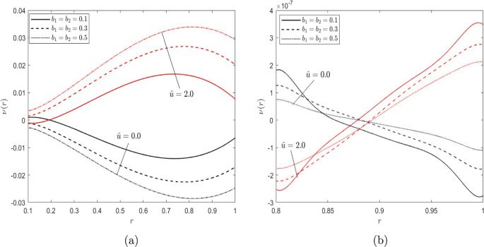
Dimensionless amplitude of EOF microrotation profiles versus the dimensionless distance r for different frequency parameter \(\alpha\) and different slippage parameters in the cases of \(c=s=1\), \(k=1.0\), \(\zeta _0=-1.0\), \(\beta =1.0\), and a \(\alpha =0.0\) (steady state), b \(\alpha =62.8\)
Fig. 8 
Dimensionless amplitude of EOF velocity profiles versus the dimensionless distance r for different zeta potential ratios of the inner to the outer cylindrical wall and different frequency parameter \(\alpha\) for the cases of \(c=0.1\), with no slip and no spin and \(s=1,\,\zeta 0=-1,\,\hat{u}=1\). The case of narrow gap \(\sigma =0.9\), \(k=10\) a \(\alpha =0.628\), b \(\alpha =62.8\)
-
(iv)
Effect of zeta potentials ratio
The electroosmosis flow arises from the interplay between the applied electric field and the electric double layer. Consequently, the wall zeta potential ratio \(\beta (=\zeta _i/\zeta _o)\) exerts a noteworthy impact on the EOF, as illustrated in Fig. 8 for various electric oscillating frequencies under the condition of a small electrokinetic width \(k=10\) and a radius ratio approaching 1 \((\sigma =0.9)\). It is important to highlight that Fig. 8 includes the case of Newtonian fluids discussed in Jian et al. [15], albeit with the inclusion of the pressure gradient. Figure 8a–b shows that for micropolar fluids, when the two cylindrical walls possess opposite charges \(\beta < 0\), the orientation of the electroosmotic flow in the microannulus is closely linked to the polarity of the charged channel wall. This finding aligns with the conclusions for Newtonian fluids drawn in [15]. Now, contemplate a special case in which \(\beta\) equals 1 and \(\sigma\) equals 0.9, indicating a minimal separation between the two cylinders. The magnitudes of velocities are primarily influenced by the frequency of electric and pressure gradient oscillations. For the lower frequency of oscillation with \(c=1\), refer to Fig. 8a, where the electroosmotic flow velocity profile closely resembles that obtained for Newtonian flow \(c=0\) by Jian et al [15]. As the oscillating frequency rises, as depicted in Figs. 8b, the velocity amplitudes for micropolar and Newtonian fluids progressively diminish and approach zero away from the two electric double layers along the cylindrical walls.
Similar to Figs. 8, 9 illustrates the profiles of EOF velocity as a function of dimensionless distance for various values of zeta potential and various parameters of electric oscillating frequency, excluding the case where the inner to outer cylindrical radius ratio is 0.1 \((\sigma =0.1)\) and the electrokinetic width is large \(k=100\). Figure 9 illustrates that as the inner cylindrical zeta potential increases, the velocity experiences a rapid rise from zero at the wall to a maximum velocity within the inner EDL region. Subsequently, the velocity diminishes with distance from the inner cylindrical wall and gradually increases within the outer EDL region. Finally, the velocity reaches zero at the outer cylindrical wall. These phenomena can be explained by the flow being propelled by electrical forces arising from the interaction between an externally applied electric field and the EDL field. In the situation where \(\beta\) equals 0 and \(\sigma\) equals 0.1, it signifies the extreme condition depicting electroosmotic flow (EOF) within a circular microchannel. The velocities predominantly concentrate in the outer electric double-layer (EDL) regions, irrespective of whether the electric oscillating frequency parameter is low or high and whether the flow is micropolar or Newtonian. Figure 7b shows that at high frequencies, the time scale for diffusion is significantly longer than the period of oscillation. As a result, there is not enough time for the flow momentum to spread extensively into the gap between the two cylindrical walls, and the variations in electroosmotic flow velocity are confined to a thin layer near the two solid surfaces.
For low and moderate frequencies up to at least \(\alpha =20\) under the condition of a small electrokinetic width \(k=10.0\) and a radius ratio approaching 1, the magnitudes of the microrotation amplitude increase with the decrease of the micropolarity parameter (Fig. 10a). For high frequencies, it increases with the increase of the micropolarity parameter (Fig. 10b). Additionally, Fig. 7 indicates that the magnitudes of the microrotation amplitude have greater values for \(\beta <0\) when compared with \(\beta >0\). When the micropolar parameter \(c=0.0\), the microrotation vanishes as expected. Figure 11 illustrates the profiles of EOF microrotation as a function of dimensionless distance for various values of zeta potential and various parameters of electric oscillating frequency, for the case where the inner to outer cylindrical radius ratio is 0.1 and the electrokinetic width is large \(k=100\). Figure 11 demonstrates that as the zeta potential increases within the inner cylinder, the magnitudes of microrotation amplitudes undergo a rapid escalation from zero at the wall to a peak microrotation within the inner electric double-layer region. Subsequently, microrotation diminishes as the distance from the inner cylindrical wall increases and gradually rises within the outer EDL region. Ultimately, microrotation returns to zero at the outer cylindrical wall. These observations can be elucidated by the flow being driven by electrical forces resulting from the interaction between an externally applied electric field and the EDL field. In cases where \(\beta\) equals 0 and 0.1 equals 0.1, this indicates an extreme condition representing electroosmotic flow within a circular microchannel. The microrotation predominantly concentrates in the outer electric double-layer regions, irrespective of whether the electric oscillating frequency parameter is low or high.
Fig. 9 
Dimensionless amplitude of EOF velocity profiles versus the dimensionless distance r for different zeta potential ratios of the inner to the outer cylindrical wall and different frequency parameter \(\alpha\) for the cases of \(c=0.1\), with no slip and no spin and \(s=1,\,\zeta _0=-1,\,\hat{u}=1\). The case of narrow gap \(\sigma =0.9\), \(k=100\) a \(\alpha =0.628\), b \(\alpha =62.8\)
Fig. 10 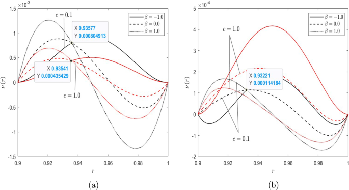
Dimensionless amplitude of EOF microrotation profiles versus the dimensionless distance r for different zeta potential ratio of the inner to the outer cylindrical wall and different frequency parameter \(\alpha\) for the cases of \(c=0.1,1\), with no slip and no spin and \(s=1,\,\zeta _o=-1,\,\hat{u}=1\). The case of narrow gap \(\sigma =0.9,\,k=10\) a \(\alpha =0.628\), b \(\alpha =62.8\)
Fig. 11 
Dimensionless amplitude of EOF microrotation profiles versus the dimensionless distance r for different zeta potential ratio of the inner to the outer cylindrical wall and different frequency parameter \(\alpha\) for the cases of \(c=0.1,1\), with no slip and no spin and \(s=1,\,\zeta _o=-1,\,\hat{u}=1\). The case of wide gap \(\sigma =0.1,\,k=100\) a \(\alpha =0.628\), b \(\alpha =62.8\)
-
(v)
Effect of time
Fig. 12 
Dimensionless EOF velocity profiles as a function of the radial distance r with no slippage for different frequency parameter \(\alpha\) and different phase \(\omega t\) in the cases of \(k=10.0\), \(s=1\), \(\hat{u}=1.0\), \(s=1.0\), \(\zeta _o=-1.0\), \(\beta =1.0\), and a \(\alpha =0.628\), b \(\alpha =62.8\)
Fig. 13 
Dimensionless EOF microrotation profiles as a function of the radial distance r with no slippage for different frequency parameter \(\alpha\) and different phase \(\omega t\) in the cases of \(k=10.0\), \(s=1\), \(\hat{u}=1.0\), \(s=1.0\), \(\zeta _o=-1.0\), \(\beta =1.0\), and a \(\alpha =0.628\), b \(\alpha =62.8\)
The variation in velocity and microrotation over time stands out as a crucial flow attribute in the context of periodic electroosmosis within a microannulus. The instantaneous velocity and microrotation profiles within a period of a time cycle are presented in Figs. 12 and 13, respectively, for different frequency parameters and for the micropolarity parameters \(c=0, 1\). These outcomes can be achieved by applying time-independent Eqs. (24–25) and the equation for time-periodic electroosmotic velocity and microrotation (14). Figures 12 and 13 show that at lower oscillating frequencies, the electric double layer (EDL) expands extensively in the vicinity of the two annulus walls. Additionally, the velocity and microrotation profiles exhibit rapid variations under the influence of the applied periodic electric field.
-
(vi)
Rate of flow and microrotation strength
Figure 14a, b depicts plots illustrating the relationship between dimensionless volume flow rate Q and the frequency parameter for various electrokinetic width k values. The plots consistently reveal that across the entire parameter \(k,c,b_1,b_2\) range, the flow rate exhibits a decreasing monotonic trend as the frequency parameter increases. With an increase in the electrokinetic width k, the rate of flow Q increases for a given value of the frequency parameter. For large values of the electrokinetic width k and a fixed frequency parameter \(\alpha\), the rate of flow Q decreases as the micropolarity parameter c increases. Conversely, for low values of k where the rate of flow may either decrease or increase, the trend is determined by the increase of micropolarity parameter c, contingent on whether the frequency parameter \(\alpha\) is less than or greater than, say, \(\alpha =5\), respectively. Figure 14b shows that augmenting the slippage parameter boosts the flow rate, whereas elevating the micropolarity parameter diminishes the flow rate. Figure 14c, d presents the rate of flow versus the radii ratio of the microannulus. For all micropolarity parameter c, s values, the flow rate Q consistently decreases as the ratio \(\sigma\) increases, and it diminishes entirely, as anticipated, when \(c\rightarrow 1\), see Fig. 14c. The plots in Fig. 14d illustrate the flow rate for different values of the zeta potential ratio. They reveal that the flow rate reaches a maximum at some point in the middle of the microannulus and then decreases to zero. The flow rate increases with the rising zeta potential ratio. Figure 15 depicts plots illustrating the relationship between dimensionless amplitude of the microrotation strength across the sectional area of the microannulus versus the frequency parameter \(\alpha\) for different values of micropolarity parameter c electrokinetic width k, and slippage parameters \(b_1, b_2\). It indicates that the amplitude of the microrotation strength increases with the widening of the electrokinetic width k. In general, the amplitude of the microrotation strength increases to a maximum at a certain value of the frequency parameter, then decreases with further increases in the frequency parameter. The amplitude of the microrotation strength increases, as expected, with the increase of the slip and spin slip parameters, see Fig. 15a–d.
-
(vii)
Electric current density
Fig. 14 
Variation of dimensionless volume flow rate Q versus a the frequency parameter \(\alpha\) for different c and k, with \(b_1=b_2=0.0\), \(\sigma =0.1\), \(\hat{u}=1.0\), \(\zeta _o=-1\), β = 1.0 b Radii ratio of the annulus \(\sigma\) for different zeta potential \(\beta\) with \(b_1=b_2=0.1\), \(\alpha =5\), \(\hat{u}=2\), \(\zeta _o=-1\), \(c=s=1\)
Fig. 15 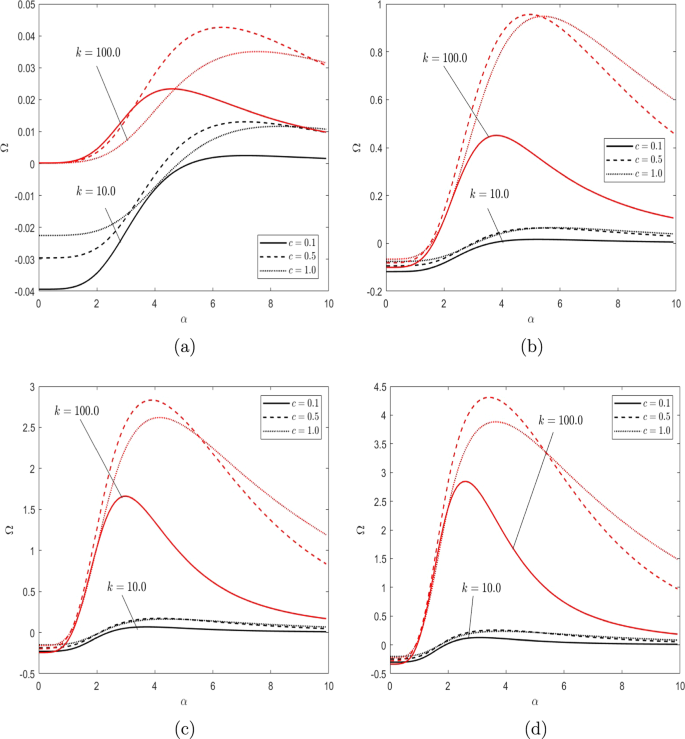
Variation of dimensionless microrotation strength across sectional area of the microannulus versus the frequency parameter \(\alpha\) for different values of c and k a \(b_1=b_2=0.0\), b \(b_1=b_2=0.1\) c \(b_1=b_2=0.3\), and d \(b_1=b_2=0.5\). Here \(\sigma =0.1\), \(\hat{u}=1\), \(s=1\), \(\zeta _o=-1\), \(\beta =1\)
Fig. 16 
Variation of dimensionless electric current density i (Eqs. (35–36)) along the microannulus versus the frequency parameter \(\alpha\) a \(b_1=b_2=0.1\), \(\beta =1\), \(R=1\) for different values of c and k b \(b_1=b_2=0.5\), \(k=2\), \(c=1\), \(R=1\) for different values of \(\beta\) c \(b_1=b_2=0.1\), \(\beta =0.5\) for different values of R and k and d \(b_1=b_2=0.1\), \(\beta =1\) for different R and k. Here \(c=0.1\), \(\hat{u}=1\), \(\zeta _o=-1\), \(\sigma =0.9\), \(s=0.1\)
Figure 16 shows the dimensionless electric current density i versus the frequency parameter \(\alpha\) for the values of electrokinetic width \(k=1,2\). It indicates that as the electrokinetic width increases, the electric current density i also increases, while an increase in micropolarity c leads to a decrease in electric current density see Fig. 16a. Figure 16b indicates that, for all values of the zeta potential ratio, the magnitude of electric current density decreases with an increasing frequency parameter. For a given value of the frequency parameter, the magnitude of electric current density increases as the zeta potential ratio decreases. For small values electrokinetic width \(k=1,2\) and \(\beta =0.5\), the magnitude of electric current density i increases with the increase of ionic Péclet number R see Fig. 16c. Figure 16d indicates that, given a fixed value of the frequency parameter with \(k=1\) and \(\beta =1\), the magnitude of electric current density i decreases as the ionic Péclet number R decreases. However, for \(k=2\), it decreases with an increase in R.


6 Conclusions
This article explores the time-periodic electrokinetic flow of a microstructured fluid using the micropolar model, as it passes through a hydrophobic microannulus. The concept of spin slip, attributed to the microrotation of the microelements, is introduced in addition to the velocity slip at the walls of the microannulus. The novelty of the presented analysis lies in studying the effect of micropolarity parameters and examining the influence of velocity slip and spin velocity slip on the time-periodic electrokinetic motion of the fluid under a pressure gradient and the imposed time-periodic electric field. The field equations of oscillating micropolar fluids, combined with the Poisson–Boltzmann equation under the Debye–Hückel approximation, have been solved. Exact expressions for the complex velocity and complex microrotation distributions are determined. The volumetric rate of flow, microrotation strength, and electric current density are then calculated and plotted for various physical parameters, with a comparison to the case of Newtonian fluids. The key observations of the current study can be summarized as follows:
-
The findings demonstrate a decline in EOF amplitudes in proximity to the two walls with an increase in micropolarity, and this trend is reversed at the center of the annulus. The periodic electric force is predominantly confined within the electric double layer (EDL) near the microannulus walls. Observable reductions in EOF amplitudes are noted beyond the EDL boundaries.
-
The amplitude of velocity increases with the increase in slippage parameters and decreases with the decrease in micropolarity.
-
In contrast to the flow rate reductions caused by the micropolarity of fluid particles, the velocity slip and spin velocity slip, when compared to Newtonian fluids, represent a counteractive mechanism that tends to augment the flow rate.
-
At significantly higher frequency parameters, the velocity is noted to approach zero at the center of the microannulus.
-
At high frequencies, there is minimal pinning observed in the central region of the microannulus for microrotation. It is interesting to note that at lower frequencies, the microrotation decreases as the electrokinetic width expands.
-
Microrotation is primarily focused on the outer regions of the electric double layer, regardless of whether the electric oscillating frequency parameter is low or high.
-
As anticipated, the amplitude of microrotation strength rises with an increase in slip and spin slip parameters.
-
The electric current density diminishes as the frequency parameter rises. Conversely, for a constant frequency parameter, the electric current density magnitude escalates as the zeta potential ratio decreases.
This study holds numerous applications in medical and engineering fields, such as the use of electroosmotic flow through a microannulus for the chemical remediation of contaminated soil. Additionally, the annulus geometry serves as an innovative microfluidic approach for effectively mixing chemical and biological fluids.
Data Availability Statement
No data are associated with the manuscript.
References
B. Lin, Microfluidics: Technologies and Applications (Elsevier, Amsterdam, 2011)
R.J. Hunter, Zeta Potential in Colloid Science (Academic press, New York, 1981)
G. Karniadakis, A. Beskok, N. Aluru, Microflows and Nanoflows: Fundamentals and Simulation (Springer, New York, 2005)
A. Bhattacharyya, J.H. Masliyah, J. Yang, Oscillating laminar electrokinetic flow in infinitely extended circular microchannels. J. Colloid Interface Sci. 261(1), 12–20 (2003)
D. Burgreen, F.R. Nakache, Electrokinetic flow in ultrafine capillary slits1. J. Phys. Chem. 68(5), 1084–1091 (1964)
D. Li, Electrokinetics in Microfluidics (Academic, New York, 2004)
J.H. Masliyah, S. Bhattacharjee, Electrokinetic and Colloid Transport Phenomena (Wiley, Hoboken, 2006)
C.L. Rice, R. Whitehead, Electrokinetic flow in a narrow cylindrical capillary. J. Phys. Chem. 69(11), 4017–4024 (1965)
S. Levine, J.R. Marriott, G. Neale, N. Epstein, Theory of electrokinetic flow in fine cylindrical capillaries at high zeta potentials. J. Colloid Interface Sci. 52, 136 (1975)
H.K. Tsao, Electro-osmotic flow through an annulus. J. Colloid Interface Sci. 225, 247 (2000)
S. Das, S. Chakraborty, Transverse electrodes for improved DNA hybridization in microchannels. AIChE J. 53, 1086 (2007)
S. Das, K. Subramanian, S. Chakraborty, Analytical investigations on the effects of substrate kinetics on macromolecular transport and hybridization through microfluidic channels. Colloids Surf. B 58, 203 (2007)
Ashraf Z. Al-Hamdan, Krishna R. Reddy, Transient behavior of heavy metals in soils during electrokinetic remediation. Chemosphere 71, 860–871 (2008)
N. Scales, R.N. Tait, Modeling electro-osmotic and pressure-drive flows in porous microfluidic devices: Zeta potential and porosity changes near the channel walls. J. Chem. Phys. 125, 094714 (2006)
Y. Jian, L. Yang, Q. Liu, Time periodic electro-osmotic flow through a microannulus. Phys. Fluids 22(4), 042001 (2010)
A. Eringen, Theory of micropolar fluids. J. Math. Mech. 16, 1–18 (1965)
Z. Ding, Y. Jian, L. Wang, L. Yang, Analytical investigation of electrokinetic effects of micropolar fluids in nanofluidic channels. Phys. Fluids 29(8), 082008 (2017)
M.K. Chaube, A. Yadav, D. Tripathi, O.A. Bég, Electroosmotic flow of biorheological micropolar fluids through microfluidic channels. Korea-Australia Rheol. J. 30(2), 89–98 (2018)
F. Karampour, A.H. Poshtiri, A. Hadizade, A study on the electroosmotic flow of micropolar fluid in a channel with hydrophobic walls. J. Braz. Soc. Mech. Sci. Eng. 44(5), 198 (2022)
M.S. Faltas, H.H. Sherief, N.M. El-Maghraby, E.F. Wanas, The electrokinetic flow of a micropolar fluid in a microtube with velocity and spin velocity slippage. Chin. J. Phys. 89, 504–27 (2023). https://doi.org/10.1016/j.cjph.2023.10.034
C. Neto, D.R. Evans, E. Bonaccurso, H.-J. Butt, V.S.J. Craig, Boundary slip in Newtonian liquids: a review of experimental studies. Rep. Prog. Phys. 68(12), 2859 (2005)
S. Jiménez Bolaños, B. Vernescu, Derivation of the Navier slip and slip length for viscous flows over a rough boundary. Phys. Fluids 29(5), 057103 (2017)
S. Gogte, P. Vorobieff, R. Truesdell, A. Mammoli, F. van Swol, P. Shah, C.J. Brinker, Effective slip on textured superhydrophobic surfaces. Phys. Fluids 17(5), 051701 (2005)
D.C. Tretheway, C.D. Meinhart, Apparent fluid slip at hydrophobic microchannel walls. Phys. Fluids 14(3), L9–L12 (2002)
V.P. Andreev, S.B. Koleshko, D.A. Holman, L.D. Scampavia, G.D. Christian, Hydrodynamics and mass transfer of coaxial jet mixer in flow injection analysis. Anal. Chem. 71, 2199 (1999)
Z. Ding, Y. Jian, L. Yang, Time periodic electroosmotic flow of micropolar fluids through microparallel channel. Appl. Math. Mech. 37(6), 769–786 (2016)
R.C. Wu, K.D. Papadopoulos, Electro-osmotic flow through porous media: cylindrical and annular models. Colloids Surf. A 161, 469 (2000)
C.C. Chang, C.Y. Wang, Starting electro-osmotic flow in an annulus and in a rectangular channel. Electrophoresis 29, 2970 (2008)
D.F. Mayano, K. Saha, G. Prakash, B. Yan, H. Kong, M. Yazdani, V.M. Rotello, nanoparticles with tunable hydrophobicity. Am. Chem. Soc. Nano 8, 6748–6755 (2014)
H.M. Park, Electrophoresis of particles with Navier velocity slip. Electrophoresis 34(5), 651–661 (2013)
C.I. Bouzigues, P. Tabeling, L. Bocquet, Nanofuidics in the Debye layer of hydrophilic and hydrophobic surface. Phys. Rev. Lett. 101(114503), 2008 (2008)
M.C.M.V. Loosdrecht, J. Lyklema, W. Norde, G. Schraa, A.J.B. Zehnder, Electrophoretic mobility and hydrophobicity as a measure to predict the initial steps of bacterial adhesion. Appl. Environ. Microbiol. 53, 1898–1901 (1987)
M. Kobayashi, An analysis on electrophoretic mobility of hydrophobic polystyrene particles with low surface charge density: effect of hydrodynamic slip. Colloid Polym. Sci. 298, 1313–1318 (2022)
S. Chakraborty, S. Das, Streaming-field-induced convective transport and its influence on the electroviscous effects in narrow fluidic confinement beyond the Debye-Hückel limit. Phys. Rev. E 77(3), 037303 (2008)
Funding
Open access funding provided by The Science, Technology & Innovation Funding Authority (STDF) in cooperation with The Egyptian Knowledge Bank (EKB).
Author information
Authors and Affiliations
Corresponding author
Rights and permissions
Open Access This article is licensed under a Creative Commons Attribution 4.0 International License, which permits use, sharing, adaptation, distribution and reproduction in any medium or format, as long as you give appropriate credit to the original author(s) and the source, provide a link to the Creative Commons licence, and indicate if changes were made. The images or other third party material in this article are included in the article's Creative Commons licence, unless indicated otherwise in a credit line to the material. If material is not included in the article's Creative Commons licence and your intended use is not permitted by statutory regulation or exceeds the permitted use, you will need to obtain permission directly from the copyright holder. To view a copy of this licence, visit http://creativecommons.org/licenses/by/4.0/.
About this article

Cite this article
Faltas, M.S., El-Sapa, S. Time-periodic electrokinetic analysis of a micropolar fluid flow through hydrophobic microannulus. Eur. Phys. J. Plus 139, 575 (2024). https://doi.org/10.1140/epjp/s13360-024-05204-0
Received:
Accepted:
Published:
DOI: https://doi.org/10.1140/epjp/s13360-024-05204-0