A geometrical representation of entanglement

Abstract

We introduce a novel geometrical approach to characterize entanglement relations in large quantum systems. Our approach is inspired by Schumacher’s singlet state triangle inequality, which used an entropy-based distance to capture the strange properties of entanglement using geometry-based inequalities. Schumacher uses classical entropy and can only describe the geometry of bipartite states. We extend his approach by using von Neumann entropy to create an entanglement monotone that can be generalized for higher-dimensional systems. We achieve this by utilizing recent definitions for entropic areas, volumes, and higher-dimensional volumes for multipartite quantum systems. This enables us to differentiate systems with high quantum correlation from systems with low quantum correlation and differentiate between different types of multipartite entanglement. It also enable us to describe some of the strange properties of quantum entanglement using simple geometrical inequalities. Our geometrization of entanglement provides new insight into quantum entanglement. Perhaps by constructing well-motivated geometrical structures (e.g., relations among areas, volumes, etc.), a set of trivial geometrical inequalities can reveal some of the complex properties of higher-dimensional entanglement in multipartite systems. We provide numerous illustrative applications of this approach, and in particular to a random sample of a thousand density matrices.

1 Introduction

Entanglement is considered the most non-classical manifestation of quantum mechanics with many strange features such as that the knowledge of the whole system does not include the best possible knowledge of its parts, or it contains correlations that are incompatible with assumptions of classical theories of physics [1,2,3]. These qualities resulted in the famous EPR paper and the idea of an alternative theory which was later ruled out by Bell’s inequality, and its experimental confirmations [4,5,6,7,8,9]. Studies of entanglement can be separated into two main categories: efforts regarding the applications of entanglement in quantum protocols and efforts concerning the fundamental questions about the nature of entanglement [10, 11].

On the applications side, it was shown that although entanglement in itself does not carry information, it can be helpful in many tasks such as the reduction of classical communication complexity [12], quantum key distribution [13], and quantum teleportation [14]. In other words, for one to perform fundamental quantum protocols, entanglement in the form of a maximally entangled state must be consumed [15].

In real-world applications, entanglement ordinarily does not come in its pure form but rather as a mixture of pure states; therefore, having a scalable way to detect and quantify entanglement can be important for quantum information processing. This was the motivation for the creation of a class of functions for quantifying entanglement known as entanglement measures, such as quantum discord [16], concurrence [17], squashed entanglement [18], operators or inequalities for detection of entanglement called entanglement wittiness such as CHSH inequality [19], and partial transpose criteria [20, 21]. All these innovative methods are geared to, and work best for bipartite systems. Furthermore, despite some efforts to generalizes these methods to multipartite systems [22,23,24], we are not aware of any efficient way to quantify and detect entanglement in high-dimensional multipartite quantum systems. We propose one small step in this direction in this manuscript.

As a guide to our construction we use traditional motivations used for most approaches. In particular, it is well accepted that any such measure must satisfy at least a set of three properties: (1) the monotonicity axiom [25]; (2) be vanishing for separable states [26]; and (3) be invariant under local unitary operators. It is interesting to note that, from the measures and witnesses that we have mentioned above, only concurrence satisfies all of these properties for bipartite systems.

Entanglement is applicable to more than just quantum information processing. In fundamental physics of entanglement, the questions are far more diverse and range from the implications of quantum entanglement and its relations to other parts of physics such as general relativity [27, 28] to deep philosophical questions related to causality in entangled systems [29] and questions regarding mathematical structure of entanglement. This latter issue is nicely captured in a quote by Bogdan Mielnik ‘What picture does one see, looking at a physical theory from a distance, so that the details disappear? Since quantum mechanics is a statistical theory, the most universal picture which remains after the details are forgotten is that of a convex set’ [30]. We take motivation from this observation in our current work where one particular interpretation of this last questions would be the possibility of the complexity of entanglement arising simply because we are not looking at it using the correct geometrical structures. We assert at a well-motivated geometry may reduce the properties of entanglement to a set of trivial geometrical properties of convex sets.

As one can guess, answering the last question is of greater importance for the foundation of quantum mechanics and our understanding of physical laws. Still, it can also be beneficial to the problems related to the application of quantum entanglement. If one can simplify the entanglement and eliminate its complexities, he will also be able to quantify and detect it. This is the motivation behind our current manuscript.

In this paper, we try to simplify the problem of entanglement by introducing entanglement monotones that play the role of information distances, areas, volumes, and higher-dimensional volumes [31, 32]. This approach enables us to distinguish separable states from entangled states by examining the geometrical differences between them. It also gives us the ability to differentiate between different types of entanglement in quantum systems. However, maybe the most interesting utility of our method would be the ability to ‘filter’ or coarse grain the entanglement in large systems by using inequalities related to higher-dimensional geometrical structures without requiring one to calculate all pairwise entanglement of nodes to determine whether a specific group of nodes in the system is entangled with the rest of the network. As an observation, we will also show that these geometrical structures will enable us to describe the specific case of monogamy of entanglement as a simple geometrical inequality. We do not claim that the geometrical relations that we have defined here can completely characterize the geometry and complexity of quantum information; nevertheless, we do show even simple geometrical constructs can describe and quantify entanglement with more utility than most of the entanglement measures that are currently in use. This can be interpreted as further evidence that by constructing a well-defined geometry, one should be able to reduce the complexity of the problem.

In Sect. 2, we will introduce our physical motivation for a new metric called the convoluted metric. Our definition is inspired by the works of Schumacher [33] and Rolkin and Rajski [34, 35]. We then prove that this metric is a valid distance measure, satisfies all the requisite properties of an entanglement monotone, and the distances $\mathcal {M}_{ij}$ created using this method are indicators of separability between nodes i, j, and the rest of the system. Later we show, for a tripartite system with at least one separable part, these distances are equivalent to squashed entanglement [22]. In Sect.  3, we will generalize these distances to areas and volumes, as well as higher-dimensional volumes using an approach introduced in [31, 32], and we show that the areas are also invariant under unitary transformations and is monotonically non-increasing under local operations and classical communication (LOCC), and are convex. In Sect. 4, we will show how this approach will offer a new way to detect entanglement beyond the bipartite definition of entanglement and apply it to some relevant applications. We conclude by suggesting a new function that might be useful for approximating entanglement content of quantum systems. The proof of each proposition will be provided in appendix.

2 Convoluted metric an entanglement monotone

Rolkin [34] and Rajski [35] introduced an information metric

$$\begin{aligned} d_{12} = \overline{A_1A_2} = H(\rho _{1|2})+H(\rho _{2|1}) \end{aligned}$$

(1)

between two random variables $A_1$ and $A_2$ with conditional probability density $\rho _{1|2}$, where $H(\rho _{1|2})$ is the usual conditional entropy. Using this metric, Schumacher [33] was able to show that geometry created by entangled states has unique geometrical features; for example, the shortest distance between points in this geometry might not be the direct distance, and this has been experimentally shown by [36] using the measurements on polarization’s of entangled photons. Inspired by his work, we introduce two different forms of distance for a random n-partite quantum network with quantum density matrix $\rho _{123...n}$ that we will define below as $D_{AB}$ and $\widetilde{D}_{AB}$. We label Hilbert spaces as A, B, ... and the von Neumann entropy as $S= -Tr(\rho \,ln \rho )$ of $\rho$ [37]. So for $\rho _{AB}$, S(AB) is the entropy of the state and S(A) is the entropy of ${{\,\mathrm{Tr}\,}}_{B}(\rho _{AB})$. Then for $\rho _{ABC}$, the entropy of register A conditioned on register B, referred to as the conditional entropy, is: $S(A|B) = S(AB) - S(B) \ .$ Using this, we define two types of information distance: For $\rho _{ABC}$, the distance $D_{AB}$ is defined as:

$$\begin{aligned} D_{AB} =&S(A|B) + S(B|A)\nonumber \\ =&S(AB) - S(B) + [S(AB) - S(A)] \nonumber \\ =&2 S(AB) - S(A) - S(B) , \end{aligned}$$

(2)

and the distance $\tilde{D}_{AB}$ is defined as follows:

$$\begin{aligned} \widetilde{D}_{AB} \equiv&S(A|BC) + S(B|AC) \nonumber \\ =&S(ABC) - S(BC) + [S(ABC) - S(AC)] \nonumber \\ =&2 S(ABC) - S(AC) - S(BC) . \end{aligned}$$

(3)

The physical motivation for defining such variables is quite simple; let us assume we have a triangle $\overline{A_1A_2A_3}$ illustrated in Fig. 1.

Fig. 1

Tripartite triangle formed by the three qubits $A_1$, $A_2$, and $A_3$

The distance of vertex $A_1$ and $A_2$ is usually a function of position of $A_1$ and $A_2$ and is independent of position of other points in our geometry. However, if we assume in our geometry this distance will also depend on the position of other vertexes then we must take this into account in our definition of distance. We call this the convoluted distance. This is a non-local effect in the sense it is a measure of the asymmetry between $A_1$ and $A_2$ with respect to extra resource of the register $A_3$.

Consequently, we define our metric $M_{AB}$ (convoluted metric) for $\rho _{ABC}$ as difference of the distances D and ${\tilde{D}}$:

$$\begin{aligned} M_{AB} \equiv&D_{AB} - \widetilde{D}_{AB} \nonumber \\ =&2S(AB) - S(A) -S(B) - [2S(ABC) - S(AC) - S(BC)] \nonumber \\ =&-2S(ABC) + 2S(AB) + S(AC) + S(BC) -S(A) - S(B) . \end{aligned}$$

(4)

As one might think for the definition, this metric $M_{AB}$ provides the means of non-separability of $\rho _{AB}$ from $\rho _C$, since it measures distance of Alice and Bob’s registers both locally and non-locally.

For any density matrix $\rho _{ABC}$, the convoluted metric $M_{AB}$ may be seen as a pseudo-metric. That is to say:

• 1. $M_{AB} = M_{BA}$,

• 2. $M_{AB} \ge 0\ \hbox {and is equal to}\ 0\$iff $\rho _{ABC}=\rho _{AB} \otimes \rho _C$,  and

• 3. $M_{AB} + M_{BC} \ge M_{AC}$.

For the special case of tripartite density matrix in the form of $\rho _{ABC}=\rho _{AB} \otimes \rho _C$, $M_{AB}$ is equal to the bipartite squashed entanglement [22] up to a constant factor. This has been shown in appendix E. In other words, one can think of this metric as geometrical representation of squashed entanglement in this case.

For the case of bipartite entanglement, it is sufficient to compare our distances to squashed entanglement and not other entanglements measures since there are many ways to write the entanglement of a bipartite system, e.g., distillable entanglement [25], entanglement cost [38], the entanglement of formation [17], relative entropy of entanglement, squashed entanglement, since it has been proved that many of these will equal to S(C) for pure states. The reason we compare it to squashed entanglement is simply because, similar to squashed entanglement, our function looks at the entanglement of A and B from the point of view of register C. In the end, however, as mentioned in the introduction, the distances and later volumes and areas, are entanglement monotones, and can be used to create different entanglement measures or witnesses.

It is easy to show that convoluted metric $M_{AB}$ is an entanglement monotone and satisfies the following properties:

• 1. $M_{AB}$ is invariant under local and global isometries,

• 2. $M_{AB}$ is non-increasing under LOCC,

• 3. $M_{AB}$ is convex.

For a given a state $\rho _{ABX}$, one could generally find many ways of decomposing it into an ensemble $\{p_{i},\rho _{i}\}_{i \in \Sigma }$. In other words, there are many ensembles whose average state is $\rho _{ABX}$. The decomposition may vary in both the number of states in the ensemble, $|\Sigma |$, and the choice of state $\rho _{i}$. This suggests an extra measure must be taken to expand the definition for mixed density matrices. Therefore, for given $\rho _{ABX}$, the convoluted metric, $M_{AB}$, for a mixed quantum density matrix is defined as follows:

$$\begin{aligned} M_{AB} \equiv \inf \{ \sum _{j} p_{j} M_{AB}(\rho ^j_{ABX}) \} \end{aligned}$$

(5)

where the infimum is taken over all possible decomposition’s of pure state density matrix $\rho ^j_{ABX}$.

Convexity is an important property for our geometrical structures. This is why we choose to make our structures convex roof monotones by adding the infimum to our definitions in Eq.  5 for mixed states. Since the set of entangled states is a convex set, it seems logical for us to make sure any structure we create is convex. The reason for this is that we are dealing with geometrical structures related to entanglement and entangled states. Additionally, convexity enables us to use many of the properties of convex structures and theorems developed for convex structures in our paper. This is a handy tool in helping us simplify the problem further and makes proving some of the properties of our functions being entanglement monotones trivial.

Now that we have proved that our metric can be a useful tool in investigating separability problem in quantum systems, we proceed by developing new geometrical features based on this metric.

3 Higher-dimensional structures

In order to study and characterize higher-dimensional entanglement networks, we are interested in coarse-graining quantum networks. One example of questions one needs to answer for coarse-graining is if we have a density matrix of the form $\rho _{ABCD}= \rho _A \otimes \rho _{BCD}$ using the distances and squashed entanglement we can only state that $\rho _{ABCD}$ is non-separable or entangled but the type of entanglement such as bipartite or tripartite needs extra calculations. For such purposes, we introduce higher-dimensional structures such as areas and volumes.

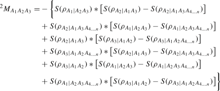
For $\rho _{A_1...A_n}$ following the procedure for distances, we define two different areas: the $Area_{A_iA_jA_k}$ and $\widetilde{\mathrm{Area}}_{A_iA_jA_k}$, which are defined as followed:

$$\begin{aligned} {\mathrm{Area}}_{A_iA_jA_k}=&-\big [S(\rho _{A_i|A_jA_k})*S(\rho _{A_j|A_iA_k})\nonumber \\&+S(\rho _{A_i|A_jA_k})*S(\rho _{A_k|A_jA_i}) \nonumber \\&+S(\rho _{A_k|A_iA_j})*S(\rho _{A_j|A_jA_k})\big ] \end{aligned}$$

(6)

$$\begin{aligned} \widetilde{\mathrm{Area}}_{A_iA_jA_k} = -\big [&S(\rho _{A_i|A_jA_k..A_n})*S(\rho _{A_j|A_iA_k...A_n}) \nonumber \\&+S(\rho _{A_i|A_jA_k...A_n})*S(\rho _{A_k|A_jA_i...A_n}) \nonumber \\&+S(\rho _{A_k|A_iA_j...A_n})*S(\rho _{A_j|A_jA_k....A_n})\big ] \end{aligned}$$

(7)

Then using this two different areas, we define our convoluted area $^2M_{A_iA_jA_k}$ for $\rho _{A_1...A_n}$ as:

$$\begin{aligned} ^2M_{A_iA_jA_k}={\mathrm{Area}}-\widetilde{{\mathrm{Area}}}, \end{aligned}$$

(8)

and later, we expand this to mixed states by taking the infimum over all possible decompositions of density matrix. Therefore, for a mixed density matrix $\rho _{A_1...A_n}$, the convoluted area $^2M_{A_iA_jA_k}$ will equal to

$$\begin{aligned} ^2M_{A_iA_jA_k}=\inf \left[ \sum _j p_j ~~{}^2{M}_{A_iA_jA_k}(\rho ^j_{A_1...A_n})\right] \ge 0 \end{aligned}$$

(9)

We conjecture that for $\rho _{A_1...A_n}$ the convoluted area ${}^2M_{A_iA_jA_k}$ is convex. Furthermore, in Appendix C we proved that this area $^2M_{A_iA_jA_k}$ satisfies the following three properties: (1) It is invariant under local unitary operators; (2) it will vanish if subsystems $A_iA_jA_k$ are separable from the rest of the system; and (3) it is non-increasing under LOCC.

We can naturally generalize this to volumes and higher-dimensional volumes using definition introduced recently in [31]. Consequently, given $\rho _{A_1...A_n}$ two type of volumes $^{(m-1)}V_{A_1A_2\ldots A_m}$ and $^{(m-1)}\widetilde{V}_{A_1A_2\ldots A_m}$ are defined as:

$$\begin{aligned} \begin{array}{ll} {}^{^{(m-1)}}\!{\mathcal V}_{A_1A_2\ldots A_m}&:= (-1)^m \displaystyle \sum _{a_1,a_2,\ldots a_m=A_1}^{A_m} \left( \frac{1+\epsilon _{a_1a_2\ldots a_m}}{2} \right) \underbrace{ S_{a_1|a_2\ldots a_{m}}S_{a_2|a_1a_3\ldots a_{m}} \ldots S_{a_{m-1}|a_1a_2\ldots a_{m\!-\!} a_{m}} }_{ \hbox { product of}\ m\ \hbox { conditional entropies}}, \end{array} \end{aligned}$$

(10)

and

$$\begin{aligned} \begin{array}{ll} {}^{^{(m-1)}}\widetilde{{\mathcal V}}_{A_1A_2\ldots A_m}&:= (-1)^m \displaystyle \sum _{a_1,a_2,\ldots a_m=A_1}^{A_m} \left( \frac{1+\epsilon _{a_1a_2\ldots a_m}}{2} \right) \underbrace{ S_{a_1|a_2\ldots a_{n}}S_{a_2|a_1a_3\ldots a_{n}} \ldots S_{a_{m-1}|a_1a_2\ldots a_{m\!-\!} a_{n}} }_{ \hbox { product of}\ m\ \hbox { conditional entropies}}. \end{array} \end{aligned}$$

(11)

This allows us to define the m-dimensional convoluted volume $^{(m-1)}M_{A_1A_2\ldots A_m}$ as:

$$\begin{aligned} ^{(m-1)}{\mathcal M}_{A_1A_2\ldots A_m} := {{}^{^{(m-1)}}\!{\mathcal V}_{A_1A_2\ldots A_m}-{}^{^{(m-1)}}\!{\widetilde{\mathcal V}}_{A_1A_2\ldots A_m}} \end{aligned}$$

(12)

and again we can expand this to mixed density matrices as:

$$\begin{aligned} ^{(m-1)}{\mathcal M}_{A_1A_2\ldots A_m} := \inf \left( \sum _j p_j ~^{(m-1)}{\mathcal M} (\rho _j)\right) \end{aligned}$$

(13)

where the infimum is taken over all possible decompositions.

Again, as conjecture we suggest that the ${}^mM_{A_iA_jA_k..A_m}$ is convex. It is also possible for these higher dimensions to show that this convoluted volume is (1) invariant under local and global isometries and (2) non-increasing under LOCC.

Now that we showed that these structures are entanglement monotones, in the next section we will examine a few applications of these entanglement monotones and highlight their potential utility.

4 Illustrative applications

4.1 Filtering the entanglement in quantum networks

Filtering the entanglement is of significant importance for quantum computing purposes in large quantum networks. One of the applications of our convoluted structures is the ability to filtering the entanglement. It is possible in future that there will be services offering cloud quantum computing. Let us assume we have a quantum cloud system of N nodes, which we call $\Omega _N$. Since these types of technologies will be used by multiple users, it is necessary to be able to filter entanglement to avoid the disruption and leakage of information from nodes being used by one user to the other. Therefore, it is essential to be able to find islands of entangled nodes that are separable from rest of system. One can rephrase this question in this way ‘is it possible to find out if a group of m nodes $\Omega _m \subseteq \Omega _N$ is entangled to the rest of systems without calculating pairwise entanglement?’. One can answer this by using the $m-1$-dimensional convoluted volumes. This can be expressed as the following observation.

Observation 1

For the density matrices $\rho _{A_1...A_N}$ to find whether a group of nodes ${A_i|i\in L}$ is entangled to the rest of system, one has to calculate the ${}^{|L|-1}M_{A_i,i \in L}$; if the systems are of form $\rho _{A_1...A_N}=\rho _{A_i,i \in L} \otimes \rho _{A_j,j\notin L}$, then ${}^{|L|-1}M_{A_i,i \in L}$ will vanish. Therefore, by using these higher-dimensional structures one can filter the entanglement in quantum network without a need to calculate all the bipartite entanglements.

4.2 Categorizing the entanglement

Second illustrative application that we want to present is the ability of these entanglement monotones to differentiate between different types of entanglement. Let us imagine we have a quantum state $\rho _{ABCD}$. While the joint quantum state of ABCD factors into a product, one for A, B, C, and D is fully separable (and so are mixtures of these products), one can have two bipartite non-separable states as $\rho _{AB} \otimes \rho _{CD}$ or tripartite non-separable state, etc. We can question, regardless of the entanglement content of these quantum systems; how can we find out what type of entanglement is present? We show here that by using convoluted structures, we can answer this question.

Observation 2

For the two density matrices $\rho _{ABCD}=\rho _{AB} \otimes \rho _{CD}$ and ${\tilde{\rho }}_{ABCD}=\rho _{ABC} \otimes \rho _{D}$ with the same entanglement content, one can easily differentiate between the type of entanglement by looking at their different geometrical structure in terms of areas,

$$\begin{aligned}&^{2}M_{ABC}(\rho )\ne 0 ~~~~M_{AB}(\rho )=M_{CD}(\rho )=0,\nonumber \\&^{2}M_{ABC}({\tilde{\rho }})= 0 ~~ ~~M_{AB}\ne 0, M_{CD}\ne 0. \end{aligned}$$

(14)

This illustrates that the type of entanglement in the $\rho$ is bipartite entanglement and ${\tilde{\rho }}$ is of tripartite nature.

4.3 Simplifying complex properties of entanglement

The third application of these structures can be the ability to simplify the complex properties of entanglement to a set of trivial geometrical features. As an example, here we show that special cases of entanglement monogamy can be reduced to a well-known trivial geometrical inequality known as Ono’s theorem [39]. Ono’s Theorem states that for a triangle ABC with acute or right angles we have

$$\begin{aligned} 27\left[ a^2+b^2-c^2\right] ^2\left[ a^2+c^2-b^2\right] ^2\left[ c^2+b^2-a^2\right] ^2 \le (4A)^6 \end{aligned}$$

(15)

Observation 3

For a state $\rho _{ABC}$, if two qubits A and B are maximally correlated they cannot be correlated at all with a third qubit C.

Proof

We will assume that for a $\rho _{ABCD}=\rho _{ABC} \otimes \rho _D$, parts A, B are maximally entangled to each other and they are also to some degree entangled to C meaning

$$\begin{aligned} M_{AB} \ne 0 \end{aligned}$$

(16)

In this case, the defined distances $D_{AC}$ and $D_{BC}$ will take their maximum value and will be equal to each other. This makes two sides of the triangle equal to each other, knowing that the max of $D_ {AB}$ can only be equal to $D_{AC}=D_{BC}$ since A and B are maximally entangled. In this case, the triangle will have acute angles. We will show this will lead to violation of Ono’s inequality; therefore, two maximally entangled qubits cannot be correlated at all with a third qubit. We know that for $\rho _{ABCD}$ our convoluted Area

$$\begin{aligned} ^2M_{ABC}=0 \end{aligned}$$

(17)

since $\rho _{ABC}$ is separable from $\rho _D$. Therefore,

$$\begin{aligned} \left[ M_{AB}^2+M_{AC}^2-M_{BC}^2\right] ^2\left[ M_{AB}^2+M_{BC}^2-M_{AC}^2\right] ^2\left[ M_{AC}^2+M_{BC}^2-M_{AB}^2\right] ^2 \le 0 \end{aligned}$$

(18)

so one or all of the terms in the left hand side of the inequality must be zero

$$\begin{aligned}&M_{AB}^2+ M_{AC}^2- M_{BC}^2 =0 \end{aligned}$$

(19)

$$\begin{aligned}&M_{BC}^2+ M_{AB}^2- M_{AC}^2 =0 \end{aligned}$$

(20)

$$\begin{aligned}&M_{BC}^2+ M_{AC}^2- M_{AB}^2 =0 \end{aligned}$$

(21)

Now using the fact that since $\rho _{AB}$ is maximally entangled and symmetric then

$$\begin{aligned} M_{AC}=M_{BC} \ne 0 \end{aligned}$$

(22)

This will reduce the equations to

$$\begin{aligned}&M_{AB}=0 \end{aligned}$$

(23)

$$\begin{aligned}&or \nonumber \\&M_{AB}^2= 2M_{AC}^2 \end{aligned}$$

(24)

but the second equation is not possible since $M_{AC}$ is the maximum value that M can take since we already assumed that A and B are maximally entangled; therefore, $M_{AB}$ must be zero which is contradiction and this proves our claim. $\square$

4.4 Approximating entanglement content of quantum systems

As the fourth and final use case, we will try to harvest these geometrical structures to approximate the entanglement content of the quantum system. The argument is that the entanglement content of a tripartite density matrix is the sum of bipartite entanglement of quantum systems and the entanglement shared between three parts; using this logic for the n-partite system, we can suggest the following. Given $\rho _{A_1...A_n}$, the entanglement content of system can be approximated by E:

$$\begin{aligned} E(\rho _{a_1a_2..a_m})&=\frac{1}{{2!}}\sum _{a_ia_j}M_{a_ia_j}\nonumber \\&\quad +\frac{1}{{3!}}\sum _{a_ia_ja_k}{}^3M_{a_ia_ja_k}+\frac{1}{{4! }}\sum _{a_ia_ja_ka_l}{}^4M_{a_ia_ja_ka_l}+... \end{aligned}$$

(25)

The coefficient are normalization factors to avoid the multiple counting. For mixed quantum density matrix,

$$\begin{aligned} \rho _{a_1a_2..a_m} =\sum _i \lambda _i \rho ^i_{a_1a_2..a_m} \end{aligned}$$

(26)

will equal to

$$\begin{aligned} E(\rho _{a_1a_2..a_m})= inf\big (\sum _n \lambda _i E(\rho ^i)\big ). \end{aligned}$$

(27)

$E(\rho )$ satisfies the following two properties: (1) It is invariant under local and global isometries; and (2) it is non-increasing under LOCC. Furthermore, $E(\rho )$ is also convex due to convexity of each of its individual parts. By way of illustration of this point, we can demonstrate that the $E(\rho )$ function can approximate the entanglement content of a quantum system. For example, we analyzed the entanglement content of quantum networks with four parts. Because we want to compare our hypothesis to concurrence (C), we generated 1000 random density matrices of form $\rho _{12} \otimes \rho _{34}$ using [40]. The entanglement content of this system would be equal to $C(\rho _{12})+ C(\rho _{34})$. Next, we calculate the values of $E(\rho _{1234})$ and normalize them by putting $E_{\rho _{\mathrm{bell}}\otimes \rho _{\mathrm{bell}}}$ equal to 2 ( we divide all the values by $\frac{E_{\rho _{\mathrm{bell}}\otimes \rho _{\mathrm{bell}}}}{2}$ ) . After this, we sorted the density matrices based on the value of concurrence and plot the values of concurrence and E. Figure 2 illustrates that E can be used to approximate the entanglement content of quantum systems.

Fig. 2

Comparison of concurrence and $E(\rho _{1234})$ for a random sample of a thousand density matrices of the form $\rho _{1234}= \rho _{12} \otimes \rho _{34}$. We normalized E by setting $E_{\rho _{\mathrm{bell}}\otimes \rho _{\mathrm{bell}}} =2$

We conjecture that replacing the von Neumann entropy with Shannon entropy in the definitions of metric and volumes, one might be able to generate an experimental lower bond for the entanglement that would be useful for applications such as quantum optics and information theory [36].

5 Conclusion

In this work, we attempted to simplify the problem of multipartite entanglement by introducing entanglement monotones that play the role of distances, areas, and higher-dimensional information volumes. This approach enables us to distinguish separable states from entangled states by examining their geometrical differences through inequalities—a sort of ‘filtering of quantum entanglement.’ To us, the most interesting utility of our method is to filter entanglement without requiring an exponentially increasing number of calculations to determine whether a specific group of nodes in the system is entangled with the rest of the network. As an observation, we also showed that these geometrical structures will enable us to describe the specific case of monogamy of entanglement as a simple geometrical inequality. We do not claim that that the geometry we have created is a complete geometry of quantum information; nevertheless, we show even such a simple geometric constructs can describe and quantify entanglement with more utility than most of the entanglement measures that are currently in use. This can be interpreted as further evidence that by constructing a well-defined geometry, one should be able to reduce the complexity of the higher-dimensional entangled systems. We suggest by exploring these higher-dimensional entropic geometries one can gain a deeper insight into some of the strange properties of entangled networks, though realizing that this approach offers but another independent glimpse into entanglement.

Appendix

In this section, we will present the proves for our proposed claims in the manuscript.

1.1 Appendix A

For any density matrix $\rho _{ABC}$, the convoluted metric $M_{AB}$ may be seen as a pseudo-metric. That is to say:

• 1.1 $M_{AB} = M_{BA}$

• 1.2 $M_{AB} \ge 0\ \hbox {and is equal to}\ 0\$iff $\rho _{ABC}=\rho _{AB} \otimes \rho _C$.

• 1.3 $M_{AB} + M_{BC} \ge M_{AC}$

Proof

• 1.1 In Eq.4, A and B are interchangeable.

• 1.2 We know from strong subadditivity of quantum entropy (SSA) inequality [41] that for tripartite separable density matrix

  $$\begin{aligned} S(\rho _{ABC})\le S(\rho _{AC})+S(\rho _{BC})-S(\rho _{C}) \end{aligned}$$

  (28)

  One can write this inequality in two different ways

  $$\begin{aligned} S(\rho _{ABC})\le S(\rho _{AC})+S(\rho _{AB})-S(\rho _{A}) \end{aligned}$$

  (29)
  $$\begin{aligned} S(\rho _{ABC})\le S(\rho _{BC})+S(\rho _{AB})-S(\rho _{B}) \end{aligned}$$

  (30)

  Now by summing up these inequalities, one will reach to

  $$\begin{aligned} S(\rho _{ABC})+ S(\rho _{ABC})\le S(\rho _{BC})+S(\rho _{AB})-S(\rho _{B})+S(\rho _{AC})+S(\rho _{AB})-S(\rho _{A}) \end{aligned}$$

  (31)

  This will lead to

  $$\begin{aligned} \big [S(\rho _{ABC})-S(\rho _{BC})\big ]+ \big [S(\rho _{ABC})-S(\rho _{AC})\big ] \le S(\rho _{AB})-S(\rho _{B})+S(\rho _{AB})-S(\rho _{A}) \end{aligned}$$

  (32)

  which is equal to

  $$\begin{aligned} \widetilde{D}_{AB} \le D_{AB}; \end{aligned}$$

  (33)

  hence, $M_{AB}$ is

  $$\begin{aligned} 0\le D_{AB}-\widetilde{D}_{AB}= M_{AB}. \end{aligned}$$

  (34)

  Furthermore, $M_{AB}$ is zero if and only if $\rho _{ABC}=\rho _{AB} \otimes \rho _C$. Since

  $$\begin{aligned} S(ABC)=&S(AB)+S(C) \nonumber \\ S(AC)=&S(A)+S(C) \nonumber \\ S(BC)=&S(B)+S(C) \end{aligned}$$

  (35)

  for $\rho _{ABC}=\rho _{AB} \otimes \rho _C$ and plugging in 35 in Eq. 4 will make $M_{AB}=0$.

• 1.3 For triangle inequality, we start with definition of $M_{AB}$

  $$\begin{aligned}&M_{AB}= S(\rho _{A|B})+S(\rho _{B|A})-S(\rho _{A|BC})-S(\rho _{B|AC}) \end{aligned}$$

  (36)
  $$\begin{aligned}&M_{AB}=2S(\rho _{AB})-2S(\rho _{ABC})+S(\rho _{BC})+S(\rho _{AC})-S(\rho _A)-S(\rho _B) \end{aligned}$$

  (37)

  Now plugging in the definition into

  $$\begin{aligned} M_{AB}+M_{BC}\ge M_{AC} \end{aligned}$$

  (38)

  and after canceling the terms, we have

  $$\begin{aligned} 2S(\rho _{AB})-2S(\rho _{ABC})+2S(\rho _{BC})-2S(\rho _B) \ge 0 . \end{aligned}$$

  (39)

  This is strong subadditivity equation [41]

  $$\begin{aligned} S(\rho _{AB})+S(\rho _{BC}) \ge S(\rho _{ABC})+S(\rho _B) \end{aligned}$$

  (40)

  and is true for any arbitrary density matrix.$\square$

For n-partite systems to show $M_{12}$ is a metric, one just needs to adjust $\rho _{3}$ to $\rho _{3...n}$.

1.2 Appendix B

Given $\rho _{ABX}$, the convoluted metric $M_{AB}$ is an entanglement monotone for detecting separability between the registers AB and X satisfies the following properties:

• 2.1 $M_{AB}$ is invariant under local and global isometries

• 2.2 $M_{AB}$ is non-increasing under LOCC

• 2.3 $M_{AB}$ is convex.

Proof

If we write the $M_{AB}$ in terms of conditional mutual information

$$\begin{aligned} M_{AB} =&-2S(ABC) + 2S(AB) + S(AC) + S(BC) -S(A) - S(B) \nonumber \\ =&[S(AB) + S(AC) -S(ABC) - S(A)] + [S(AB) + S(BC) -S(ABC) - S(B)] \nonumber \\ =&I(B:C|A) + I(A:C|B) \end{aligned}$$

(41)

• 2.1 von Neumann entropy is invariant under unitary operation; therefore, $M_{AB}$ is invariant under unitary operation.

• 2.2 Conditional mutual information is non-increasing under LOCC [22]; therefore, $M_{AB}$ is non-increasing under LOCC.

• 2.3 Conditional mutual information is convex [22]; therefore, $M_{AB}$ is convex since the sum of two convex functions is also convex.

$\square$

1.3 Appendix C

Given $\rho _{A_1...A_n}$, the $^2M_{A_iA_jA_k}$ satisfies the following properties:

• 3.1 is invariant under local and global isometries

• 3.2 is convex.

• 3.3 is non-increasing under LOCC.

Proof

• 3.1 The von Neumann entropy is invariant under unitary operation; therefore, $^2M_{A_i A-j A_k}$ is invariant under unitary operation.

• 3.2 By adding and subtracting the terms

  $$\begin{aligned}&S(\rho _{A_1|A_2A_3})*S(\rho _{A_2|A_1A_3A_{4 ....n}}) \end{aligned}$$

  (42)
  $$\begin{aligned}&S(\rho _{A_2|A_1A_3})*S(\rho _{A_3|A_1A_2A_{4 ....n}}) \end{aligned}$$

  (43)
  $$\begin{aligned}&S(\rho _{A_3|A_1A_2})*S(\rho _{A_1|A_2A_3A_{4 ....n}}) \end{aligned}$$

  (44)

  To $^2M_{A_1A_2A_3}$ make it equal to

  

  (45)

  Then we rewrite this as

  $$\begin{aligned} ^2M_{A_1A_2A_3}=&-\big [S(\rho _{A_1|A_2A_3})+S(\rho _{A_3|A_1A_2A_{4 ....n}})\big ]*\big [S(\rho _{A_2|A_1A_3})-S(\rho _{A_2|A_1A_3A_{4 ....n}})\big ]\nonumber \\&- \big [S(\rho _{A_3|A_1A_2})+S(\rho _{A_2|A_1A_3A_{4 ....n}})\big ]*\big [S(\rho _{A_1|A_2A_3})-S(\rho _{A_1|A_2A_3A_{4 ....n}})\big ] \nonumber \\&- \big [S(\rho _{A_2|A_1A_3})+S(\rho _{A_1|A_2A_3A_{4 ....n}})\big ]*\big [S(\rho _{A_3|A_1A_2})-S(\rho _{A_3|A_1A_2A_{4 ....n}})\big ] \end{aligned}$$

  (46)

  One can express this in terms of conditional mutual information as

  $$\begin{aligned} ^2M_{A_1A_2A_3}=&\big [I(A_1;A_2A_3)+I(A_3;A_1A_2A_{4 ....n})-S(A_1)-S(A_3)\big ]*\big [I(A_2;A_{4 ....n}|A_1A_3)\big ]\nonumber \\&+ \big [I(A_3;A_1A_2)+I(A_2;A_1A_3A_{4 ....n})-S(A_3)-S(A_2)\big ]*\big [I(A_1;A_{4 ....n}|A_2A_3)\big ] \nonumber \\&+ \big [I(A_2;A_1A_3)+I(A_1;A_2A_3A_{4 ....n})-S(A_1)-S(A_2)\big ]*\big [I(A_3;A_{4 ....n}|A_1A_3)\big ] \end{aligned}$$

  (47)

  Now since we know subsystems $A_iA_jA_k$ is separable from the rest of the system $^2M_{A_iA_jA_k}$ will equal to zero due to $I(A_i;A_{4 ....n}|A_jA_k)=0$.

• 3.3 To prove that $^2M_{A_1A_2A_3}$ is non-increasing under LOCC, we have to use the proposition by [22]

Proposition 1

A convex function f does not increase under LOCC if and only if

• a) f is invariant under local unitary operators

• b) if f satisfies

  $$\begin{aligned} f\left( \sum _i p_i \rho _{AB}^i\otimes |i\rangle x \langle i| \right) =\sum _i p_if(\rho _{AB}^i). \end{aligned}$$

  (48)

Since $^2M_{A_1A_2A_3}$ satisfies both of these, then it is non-increasing under LOCC.

1.4 Appendix D

Given $\rho _{A_1...A_n}$, the $E(\rho )$ satisfies the following properties:

• 6.1 $E(\rho )$ is invariant under local and global isometries;

• 6.2 $E(\rho )$ is non-increasing under LOCC; and

• 6.3 $E(\rho )$ is convex.

Proof

• 1. $E(\rho )$ is invariant under local unitary operators due to $^mM_{A_i...A_m}$ being invariant under local unitary operators.

• 2. From our previous discussions, we know that $^mM_{A_i...A_m}$ are non-increasing under LOCC, and we know that sum of non-increasing terms will also be non-increasing under LOCC. Then $E(\rho )$ is non-increasing under LOCC.

1.5 Appendix E

For a given state $\rho _{AB}$, squashed entanglement is given by

$$\begin{aligned} E_{sq}(\rho _{AB}) = \frac{1}{2} inf I(A : B|E), \end{aligned}$$

(49)

with

$$\begin{aligned} I(A:B|E)=S(AE)+S(BE)-S(ABE)-S(E). \end{aligned}$$

(50)

It is obvious from the equation above that $I(A:B|E)= I(B:A|E)$. We have stated that if C is separable from AB our method will give answer similar to squashed entanglement, this is because the degree of entanglement of A and B in this case will equal to entanglement of the $\rho _{AC}$ part with $\rho _{B}$, or the $\rho _{BC}$ part with$\rho _{C}$. In appendix B, we have shown that

$$\begin{aligned} M_{AB}&= -2S(ABC) + 2S(AB) + S(AC) + S(BC) -S(A) - S(B) \\&= [S(AB) + S(AC) -S(ABC) - S(A)] + [S(AB) + S(BC) -S(ABC) - S(B)] \\&= I(B:C|A) + I(A:C|B). \end{aligned}$$

If we write this for either $M_{AC}$ or $M_{BC}$ after applying our convex roof method, we will simply get a constant number multiplied by Eq. 49, which means $M_{AC}$ multiplied by value of squashed entanglement. The motivation we choose to mention getting result similar to squashed entanglement is the reason we compare it to squashed entanglement is simply because, similar to squashed entanglement our function look at entanglement of A and B from point of view of register C.

References

R. Horodecki, P. Horodecki, M. Horodecki, K. Horodecki, Rev. Mod. Phys. 81, 865 (2009)
P. Horodecki, R. Horodecki, Phys. Lett. A 194, 147 (1994)
P. kurzynski and D. Kaszlikowski, Information-theoretic metric as a tool to investigate nonclassical correlations. Phys. Rev. A 89, 012103 (2014)
A. Einstein, B. Podolsky, N. Rosen, Can quantum mechanical description of physical reality be considered complete? Phys. Rev. 47, 777 (1935)
J.S. Bell, On the Einstein–Podolsky–Rosen paradox. Physics 1, 195 (1964)
A. Aspect, P. Grangier, G. Roger, Experimental tests of realistic local theories via Bell’s theorem. Phys. Rev. Lett. 47, 460 (1981)
B. Hensen et al., Loophole-free Bell inequality violation using electron spins separated by 1.3 kilometres. Nature (London) 526, 682 (2015)
M. Giustina et al., Significant-loophole-free test of Bell’s theorem with entangled photons. Phys. Rev. Lett. 115, 250401 (2015)
L.K. Shalm et al., Strong loophole-free test of local realism. Phys. Rev. Lett. 115, 250402 (2015)
M.A. Nielsen, I, L. Chuang, Quantum Computation and Quantum Information (Cambridge University Press, Cambridge, 2000)
M.M. Wilde, Quantum Information Theory, 2nd edn. (Cambridge University Press, Cambridge, 2017)
R. Cleve, H. Buhrman. arXiv:quant-ph/9704026 (1997)
A.K. Ekert, Phys. Rev. Lett. 67, 661 (1991)
C.H. Bennett, G. Brassard, C. Crepeau, R. Jozsa, A. Peres, W.K. Wootters, Phys. Rev. Lett. 70, 1895 (1993)
X. Wang, M.M. Wilde, Cost of quantum entanglement simplified. Phys. Rev. Lett. 125, 040502 (2020)
H. Ollivier, W.H. Zurek, Phys. Rev. Lett. 88, 017901 (2001)
S. Hill, W.K. Wootters, Entanglement of a pair of quantum bits. Phys. Rev. Lett. 78, 5022 (1997)
M. Christandl, A. Winter, Squashed entanglement: an additive entanglement measure. J. Math. Phys. 45, 3, 829–840 (2004). https://doi.org/10.1063/1.1643788
J.F. Clauser, M.A. Horne, A. Shimony, R.A. Holt, Proposed experiment to test local hidden-variable theories. Phys. Rev. Lett. 23(15), 880–4 (1969)
R. Simon, Peres-Horodecki separability criterion for continuous variable systems. Phys. Rev. Lett. 84(12), 2726–2729 (2000)
A. Peres, Separability criterion for density matrices. Phys. Rev. Lett. 77, 1413–1415 (1996)
D. Yang, K. Horodecki, M. Horodecki, P. Horodecki, J. Oppenheim, W. Song, Squashed entanglement for multipartite states and entanglement measures based on the mixed convex roof. IEEE Trans. Inf. Theory 55(7), 3375–3387 (2009)
F. Mintert, M. Kus, A. Buchleitner, Concurrence of mixed multipartite quantum states. Phys. Rev. Lett. 95, 260502 (2005)
C.C. Rulli, M.S. Sarandy, Global quantum discord in multipartite systems. Phys. Rev. A 84, 042109 (2011)
C.H. Bennett, D.P. DiVincenzo, J.A. Smolin, W.K. Wootters, Phys. Rev. A 54, 3824 (1996)
G. Vidal, J. Mod. Opt. 47, 355 (2000)
X.L. Qi, Does gravity come from quantum information? Nat. Phys. 14, 984–987 (2018)
M. Van Raamsdonk, Building up space-time with quantum entanglement. Gen. Relativ. Gravit. 42, 2323–2329 (2010)
P.M. Näger, The causal problem of entanglement. Synthese 193(4), 1127–1155 (2016)
I. Bengtsson, K. Zyczkowski, Geometry of Quantum States: An Introduction to Quantum Entanglement (Cambridge University Press, Cambridge, 2017)
W.A. Miller, S.M. Aslmarand, P.M. Alsing, V.S. Rana, Geometric measures of information for quantum state characterization. Ann. Math. Sci. Appl. 4(2), 395–409 (2019)
S.M. Aslmarand, W.A. Miller, V.S. Rana, P.M. Alsing, Quantum reactivity: an indicator of quantum correlation. Entropy 22(1), 6 (2020)
B.W. Schumacher, Information and quantum nonseparability. Phys. Rev. A 44, 7047 (1991)
V.A. Roklin, Lecture on the entropy theory of measure-preserving transformations. Russ. Math. Surv. 22, 152 (1967)
C. Rajski, A metric space of discrete probability distributions. Inf. Control 4, 373 (1961)
T. Rezaei et al., Experimental realization of Schumacher’s information geometric Bell inequality. Phys. Lett. A 405, 127444 (2021)
J. Von Neumann, Mathematische grundlagen der quantenmechanik, vol. 38 (Springer, Berlin, 2013)
P.M. Hayden, M. Horodecki, B.M. Terhal, The asymptotic entanglement cost of preparing a quantum state. J. Phys. A: Math. Gen. 34(35), 6891 (2001)
T. Ono, Problem 4417. Intermed. Math. 21, 14 (1914)
N. Johnston. QETLAB: A MATLAB toolbox for quantum entanglement, version 0.9. http://www.qetlab.com, January 12, 2016. https://doi.org/10.5281/zenodo.44637
E.H. Lieb, M.B. Ruskai, Proof of the strong subadditivity of quantum-mechanical entropy. J. Math. Phys. 14(12), 1938–1941 (1973)
Acknowledgements
SMA would like to thank Ian George for his suggestions and helpful discussions. WAM would like thank support from the Air Force Office of Scientific Research, Air Force Research Laboratory’s Information Directorate as well as L3Harris. This research was supported in part by the Air Force Research Laboratory Information Directorate, through the Air Force Office of Scientific Research Summer Faculty Fellowship Program®, Contract Numbers \(\#FA8750-15-3-6003\), \(\#FA9550-15-0001\) and \(\#FA9550-20-F-0005\), AFOSR/AOARD Grant \(\#FA23861714070\), AFOSR/DURIP Grant \(\#FA95501910389\) and support from L3Harris. PMA for this work would like thank support from the Air Force Office of Scientific Research. DA is support by AFOSR Grant FA2386-21-1-0089, NRF-2020M3E4A1080031 and MSIT/IITP2021-0-01810. Any opinions, findings, conclusions, or recommendations expressed in this material are those of the author(s) and do not necessarily reflect the views of AFRL.
Author information
Authors and Affiliations
Corresponding author