Improved parallel matrix multiplication using Strassen and Urdhvatiryagbhyam method

Abstract

The current milieu, encourages rapid growth of wireless communication, multimedia applications, robotics and graphics to have efficient utilization of resources with high throughput and low power digital signal processing (DSP) systems. In an aggregate DSP system ranging from audio/video signal processing to wireless sensor networks, floating point matrix multiplication is used in wide scale in most of the fundamental processing units. Hardware implementation of floating-point matrix multiplication demands a colossal number of arithmetic operations that alter speed and consuming more area and power. DSP systems essentially uses two techniques to reduce dynamic power consumption:—they are pipelining and parallel processing that needs high performance processing element with less area and low power in diverse scientific computing applications. However, number of adders and multipliers used in the design of floating-point unit also increases subsequently. The adders and multipliers are the most area, delay and power consuming data path elements in the processing unit. The arithmetic level reduction of delay, power and area in the processing element is performed by the selection of appropriate adders and multipliers. This article proposes a parallel multiplication architecture using Strassen and UrdhvaTiryagbhyam multiplier, which involves design of efficient parallel matrix multiplication with flexible implementation of FPGA (Field Programmable Gate Array) device to analyse the computation and area. The design incorporates scheduling of blocks, operations on processing elements, block size determination, parallelization and double buffering for storage of matrix elements.

1 Introduction

Floating point matrix multiplication is a building block for many linear algebra kernels (Zhou and Prassana 2008). Multiplication is a complex arithmetic operation which is reflected in its relatively high power dissipation, high signal propagational delay, and large area requirement. Hence an efficient multiplier design has become a significant part in VLSI (Very Large Scale Integration) system design (Chetan et al. 2020; Singh and Tarunkumar 2015). The overall performance of the processing system is determined by the performance of the multiplier. By using an efficient architecture for floating point matrix multiplication improves the computation complexity of the system (Sonawane et al. 2009). Multipliers are the elemental processing elements hardly in all DSP systems (Palacios et al. 1992) from multimedia (Kalaiselvi 2010) to high-speed wireless communication systems (Shen and Chen 2008). Implementations of high performance matrix operations are required in many complex algorithms in video processing applications (Kang 2007), image (Prabhune et al. 2017) and digital signal processing (Qasim et al. 2010). Based on the computational applications and performance of the system, many algorithms have been designed for matrix multiplication (Thabet and Al-Ghuribi 2012). Though there are two techniques to reduce dynamic power consumption wherein, pipelining technique reduces critical path delay and parallel processing technique replicates the hardware components to increase the performance (Li and Pan 2001).There has been wide work for matrix multiplication on parallel algorithms. Two classical algorithms Cannon’s (Cannon 1969) and Fox’s (Fox and Otto 1987) are designed in which, each processor holds consecutive blocks of data based on a square processor grid with a block data distribution. input matrices are partitioned into square blocks. All sub blocks are processed by rolling and step upward procedure (Amrutha et al. 2015). The blocks on one processor are either broad cast to the other processor or transferred to its adjacent processors in the same row throughout the iteration (Sajish et al. 2005). Blocking refers to the partitioning the matrices into smaller sub matrices. The design decision includes schedules operations, determining block sizes and determining which operations are performed in parallel (Khayyat and Manjikian 2014). Parallel universal matrix multiplication algorithm (PUMMA) which provides two-dimensional block cyclic data decomposition for Fox’s algorithm (Choi et al. 1994). Distribution–Independent Matrix Multiplication Algorithm (DIMMA) (Choi 1997) combines pipeline communication and LCM block concept to achieve the maximum performance and the Scalable Universal Matrix Multiplication Algorithm (SUMMA) for distributed memory concurrent computers (Geijn and Watts 1998a). The blocks are broadcast based on flexible broadcast- multiply- roll algorithm; the computation and communication on the processor are overlapped. Cache-based architecture (Matam et al. 2013) and Dynamic Random Access Memory (DRAM) model (Matam and Prasanna 2013) improve the performance with respect to Energy × Area × Time (EAT). A parallelized sequential algorithm on a linear array of processors, which supports massive volume of data transfer on a pipeline optical bus (Li and Pan 2001).In rank-1 update algorithm, the sub block of matrices are obtained by multiplying two panels of matrices and handle arbitrary sizes matrices (Kumar et al. 2010).A brief discussion on various techniques and its implementation to improve the performance in block matrix multiplication is shown in Table 1

Table 1 Detailed literature survey on block matrix multiplication

Concisely, it is observed that the execution time and area are two impediments that are to be looked out to enhance the overall performance of the system. The main aim of this work is to form a novel architecture for floating point matrix multiplication known as block matrix multiplication based on Strassen and UrdhvaTiryagbhyam multiplier using parallel processing. In the above said technique, the computation unit reads its inputs to perform the matrix block multiplication and writes its output to the memory. The block multiplication is executed in the computation unit where the parallelism is implemented. Scheduling assigns multiple arithmetic operations to the processing unit over a same time slot. The system efficiency is augmented by reusing the data for the ensuing operation.

In this paper, an improved algorithm for block matrix multiplication is developed to reduce the area. For this a fusion of Strassen and UrdhvaTiryagbhyam multiplier is used through parallel processing. The Parameters such area, delay, PEs, GFLOPs, LUTs, computation time, slices, IOBs and frequency have been studied using Xilinx 13.5 simulating tool and implemented in virtex-5 FPGA.

1.1 Conventional method

The standard method to achieve matrix multiplication involves O(N³) arithmetic operation. In 1969, Volker Strassen proposed matrix multiplication algorithm based on divide and conquer approach, which divides the matrices into sub matrices of equal size (Strassen 1969). Howbeit, it is faster than classical matrix multiplication scheme but necessitates fewer multiplication of matrix elements. A 2 × 2 matrix multiplication requires solely ‘7’ multiplications and ‘18’ additions or subtraction in lieu of ‘8’ multiplications and ‘4’ additions to have in the classical method. The algorithm is applied recursively for large matrices on four blocks at a time, yielding a complexity of O (N^log₂⁷) ~ O (N^2.81) which serves as a main algorithm to break the N³ barrier.

Let X and Y be two input matrices of size 4 × 4 with ‘Z’ as the output matrix of dimension 4 × 4. Matrix X is divided into sub matrices X₀, X₁.X₂ and X₃ of dimension 2 × 2 and matrix Y is divided into sub-matrices Y₀, Y₁, Y₂ and Y₃ of size 2 × 2. Let the product matrix be subdivided into Z₀, Z₁, Z₂ and Z₃ of dimension 2 × 2.

Let $X= \left(\begin{array}{ccc}{X}_{11}& {X}_{12}& \begin{array}{cc}{X}_{13}& {X}_{14}\end{array}\\ {X}_{21}& {X}_{22}& \begin{array}{cc}{X}_{23}& {X}_{24}\end{array}\\ \begin{array}{c}{X}_{31}\\ {X}_{41}\end{array}& \begin{array}{c}{X}_{32}\\ {X}_{42}\end{array}& \begin{array}{cc}\begin{array}{c}{X}_{33}\\ {X}_{43}\end{array}& \begin{array}{c}{X}_{34}\\ {X}_{44}\end{array}\end{array}\end{array}\right) Y= \left(\begin{array}{ccc}{Y}_{11}& {Y}_{12}& \begin{array}{cc}{Y}_{13}& {Y}_{14}\end{array}\\ {Y}_{21}& {Y}_{22}& \begin{array}{cc}{Y}_{23}& {Y}_{24}\end{array}\\ \begin{array}{c}{Y}_{31}\\ {Y}_{41}\end{array}& \begin{array}{c}{Y}_{32}\\ {Y}_{42}\end{array}& \begin{array}{cc}\begin{array}{c}{Y}_{33}\\ {Y}_{43}\end{array}& \begin{array}{c}{Y}_{34}\\ {Y}_{44}\end{array}\end{array}\end{array}\right)Z= \left(\begin{array}{ccc}{Z}_{11}& {Z}_{12}& \begin{array}{cc}{Z}_{13}& {Z}_{14}\end{array}\\ {Z}_{21}& {Z}_{22}& \begin{array}{cc}{Z}_{23}& {Z}_{24}\end{array}\\ \begin{array}{c}{Z}_{31}\\ {Z}_{41}\end{array}& \begin{array}{c}{Z}_{32}\\ {Z}_{42}\end{array}& \begin{array}{cc}\begin{array}{c}{Z}_{33}\\ {Z}_{43}\end{array}& \begin{array}{c}{Z}_{34}\\ {Z}_{44}\end{array}\end{array}\end{array}\right)$

Using Strassen algorithm, the above matrix is divided into sub matrices as follows:

X= $\left(\begin{array}{c}\begin{array}{cc}{X}_{0}& {X}_{1}\end{array}\\ \begin{array}{cc}{X}_{2}& {X}_{3}\end{array}\end{array}\right)$ ; Y= $\left(\begin{array}{c}\begin{array}{cc}{Y}_{0}& {Y}_{1}\end{array}\\ \begin{array}{cc}{Y}_{2}& {Y}_{3}\end{array}\end{array}\right)$ and Z = $\left(\begin{array}{c}\begin{array}{cc}{Z}_{0}& {Z}_{1}\end{array}\\ \begin{array}{cc}{Z}_{2}& {Z}_{3}\end{array}\end{array}\right)$

$$\left(\begin{array}{c}\begin{array}{cc}{X}_{0}& {X}_{1}\end{array}\\ \begin{array}{cc}{X}_{2}& {X}_{3}\end{array}\end{array}\right)\times \left(\begin{array}{c}\begin{array}{cc}{Y}_{0}& {Y}_{1}\end{array}\\ \begin{array}{cc}{Y}_{2}& {Y}_{3}\end{array}\end{array}\right)= \left(\begin{array}{cc}{X}_{0}{Y}_{0}+{X}_{1}{Y}_{2}& {X}_{0}{Y}_{1}+{X}_{1}{Y}_{3}\\ {X}_{2}{Y}_{0}+{X}_{3}{Y}_{2}& {X}_{2}{Y}_{1}+{X}_{3}{Y}_{3}\end{array}\right)$$

$$\left. {\begin{array}{*{20}c} {{\text{Z}}_{0} = {\text{X}}_{0} .{\text{Y}}_{0} + {\text{X}}_{1} .{\text{Y}}_{2} } \\ {{\text{Z}}_{1} = {\text{X}}_{0} .{\text{Y}}_{1} + {\text{X}}_{1} .{\text{Y}}_{3} } \\ {{\text{Z}}_{2} = {\text{X}}_{2} .{\text{Y}}_{0} + {\text{X}}_{3} .{\text{Y}}_{2} } \\ {{\text{Z}}_{3} = {\text{X}}_{2} .{\text{Y}}_{1} + {\text{X}}_{3} .{\text{Y}}_{3} } \\ \end{array} } \right\}$$

(1)

where ${X}_{0 }= \left(\begin{array}{c}\begin{array}{cc}{X}_{11}& {X}_{12}\end{array}\\ \begin{array}{cc}{X}_{21}& {X}_{22}\end{array}\end{array}\right)$; ${Y}_{0 }= \left(\begin{array}{c}\begin{array}{cc}{Y}_{11}& {Y}_{12}\end{array}\\ \begin{array}{cc}{Y}_{21}& {Y}_{22}\end{array}\end{array}\right)$ and Z₀ $= \left(\begin{array}{c}\begin{array}{cc}{Z}_{11}& {Z}_{12}\end{array}\\ \begin{array}{cc}{Z}_{21}& {Z}_{22}\end{array}\end{array}\right)$

${X}_{1 }= \left(\begin{array}{c}\begin{array}{cc}{X}_{13}& {X}_{14}\end{array}\\ \begin{array}{cc}{X}_{23}& {X}_{24}\end{array}\end{array}\right)$; ${Y}_{1 }= \left(\begin{array}{c}\begin{array}{cc}{Y}_{13}& {Y}_{14}\end{array}\\ \begin{array}{cc}{Y}_{23}& {Y}_{24}\end{array}\end{array}\right)$ and Z₁ $= \left(\begin{array}{c}\begin{array}{cc}{Z}_{13}& {Z}_{14}\end{array}\\ \begin{array}{cc}{Z}_{23}& {Z}_{24}\end{array}\end{array}\right)$

${X}_{2 }= \left(\begin{array}{c}\begin{array}{cc}{X}_{31}& {X}_{32}\end{array}\\ \begin{array}{cc}{X}_{41}& {X}_{42}\end{array}\end{array}\right)$; ${Y}_{2 }= \left(\begin{array}{c}\begin{array}{cc}{Y}_{31}& {Y}_{32}\end{array}\\ \begin{array}{cc}{Y}_{41}& {Y}_{42}\end{array}\end{array}\right)$ and Z₂ $= \left(\begin{array}{c}\begin{array}{cc}{Z}_{13}& {Z}_{14}\end{array}\\ \begin{array}{cc}{Z}_{23}& {Z}_{24}\end{array}\end{array}\right)$

${X}_{3 }= \left(\begin{array}{c}\begin{array}{cc}{X}_{33}& {X}_{34}\end{array}\\ \begin{array}{cc}{X}_{43}& {X}_{44}\end{array}\end{array}\right)$; ${Y}_{3 }= \left(\begin{array}{c}\begin{array}{cc}{Y}_{33}& {Y}_{34}\end{array}\\ \begin{array}{cc}{Y}_{43}& {Y}_{44}\end{array}\end{array}\right)$ and Z₃ $= \left(\begin{array}{c}\begin{array}{cc}{Z}_{33}& {Z}_{34}\end{array}\\ \begin{array}{cc}{Z}_{43}& {Z}_{44}\end{array}\end{array}\right)$

Consider that the partial product matrix P is obtained as, from Eq. (1)

P = X₀. Y_0,where P = $\left(\begin{array}{c}\begin{array}{cc}{P}_{11}& {P}_{12}\end{array}\\ \begin{array}{cc}{P}_{21}& {P}_{22}\end{array}\end{array}\right)$i.e.$\left(\begin{array}{c}\begin{array}{cc}{P}_{11}& {P}_{12}\end{array}\\ \begin{array}{cc}{P}_{21}& {P}_{22}\end{array}\end{array}\right)$ = $\left(\begin{array}{c}\begin{array}{cc}{X}_{11}& {X}_{12}\end{array}\\ \begin{array}{cc}{X}_{21}& {X}_{22}\end{array}\end{array}\right)$ . $\left(\begin{array}{c}\begin{array}{cc}{Y}_{11}& {Y}_{12}\end{array}\\ \begin{array}{cc}{Y}_{21}& {Y}_{22}\end{array}\end{array}\right)$

The partial products are generated using Eq. (2)

$$\left. {\begin{array}{*{20}c} {{\text{P}}_{{1}} = \left( {{\text{X}}_{{{11}}} + {\text{X}}_{{{22}}} } \right).\left( {{\text{Y}}_{{{11}}} + {\text{Y}}_{{{22}}} } \right)\;\;} \\ {{\text{P}}_{{2}} = \left( {{\text{X}}_{{{21}}} + {\text{X}}_{{{22}}} } \right).{\text{Y}}_{{{11}}} \;\;\;\;\;\;\;\;\;\;\;\;} \\ {{\text{P}}_{{3}} = {\text{X}}_{{{11}}} .\left( {{\text{Y}}_{{{12}}} - {\text{Y}}_{{{22}}} } \right)\;\;\;\;\;\;\;\;\;\;\;\;\;} \\ {{\text{P}}_{{4}} = {\text{X}}_{{{22}}} .\left( {{\text{Y}}_{{{21}}} - {\text{Y}}_{{{11}}} } \right)\;\;\;\;\;\;\;\;\;\;\;\;\;} \\ {{\text{P}}_{{5}} = \left( {{\text{X}}_{{{11}}} + {\text{X}}_{{{12}}} } \right).{\text{Y}}_{{{22}}} \;\;\;\;\;\;\;\;\;\;\;\;\;} \\ {{\text{P}}_{{6}} = \left( {{\text{X}}_{{{21}}} - {\text{X}}_{{{11}}} } \right).\left( {{\text{Y}}_{{{11}}} + {\text{Y}}_{{{12}}} } \right)\;\;} \\ {{\text{P}}_{{7}} = \left( {{\text{X}}_{{{12}}} - {\text{X}}_{{{22}}} } \right).\left( {{\text{Y}}_{{{21}}} + {\text{Y}}_{{{22}}} } \right)\;\;} \\ \end{array} } \right\}$$

(2)

Final matrix multiplication products are obtained as follow using Eq. (2)

$$\left. {\begin{array}{*{20}c} {{\text{P}}_{{{11}}} = {\text{P}}_{{1}} + {\text{P}}_{{4}} - {\text{P}}_{{5}} + {\text{P}}_{{7}} \;} \\ {{\text{P}}_{{{12}}} = {\text{P}}_{{3}} + {\text{P}}_{{5}} \;\;\;\;\;\;\;\;\;\;\;\;\;} \\ {{\text{P}}_{{{21}}} = {\text{P}}_{{2}} + {\text{P}}_{{4}} \;\;\;\;\;\;\;\;\;\;\;\;\;} \\ {{\text{P}}_{{{22}}} = {\text{P}}_{{1}} - {\text{P}}_{{2}} + {\text{P}}_{{3}} + {\text{P}}_{{6}} \;} \\ \end{array} } \right\}$$

(3)

From Eq. (2) its observed, to compute the result for a second- order matrix, Strassen’s algorithm needs only ‘7’ multiplication tasks, at the same time the conventional algorithm comprises ‘8’ multiplications.

According to Strassen algorithm for a nth order matrix, the number of multiplications required is given by,

$$P\left(n\right)=7 P\left(\frac{n}{2}\right)$$

(4)

where ‘7’ is the number of multiplication operation and $P\left(\frac{n}{2}\right)$ is the multiplication function of sub matrices of dimension $\frac{n}{2}\times \frac{n}{2}$

The time complexity of Strassen algorithm is represented as

$$T\left(n\right)=7P\left(\frac{n}{2}\right)+m{n}^{2} for\, n\ge 2$$

(5)

Adding matrix, yields ${n}^{2}$ steps, where c is a fixed constant value. By applying Masters Theorem Eq. (5) it is rewritten as,

$$T\left(n\right)=O\left({7}^{{log}_{{2}^{n}}}\right)=O\left({n}^{{log}_{{2}^{7}}}\right)= \mathrm{O }({n}^{2.81} )$$

(6)

The time complexity of Strassen algorithm is O (${n}^{2.81}$), which is better than conventional algorithm. For a common method to work out the product of ‘2’ 2 × 2 matrices, it takes ‘8’ multiplication process. The time complexity of n^th order matrix is given as,

$$O\left({n}^{{log}_{{2}^{8}}}\right)=O({n}^{3})$$

(7)

1.2 UrdhvaTiryagbhyam method

The word “Vedic” is imitated from the word “Veda” which means the store house of all knowledge (Jagadguru Swami Sri Bharati KrsnaTirthaji Maharaja 1985). Application of sutras saves lot of time and effort in solving problems, compared to the formal method.The utmost significant and multifaceted portion in the floating point multiplication is mantissa multiplication. Compared to addition operation multiplication requires more time. It consumes more area and time as the number of bits increases. In terms of area and delay UrdhvaTiryagbhyam algorithm is the best algorithm for binary multiplication. The partial products generated are added in ripple fashion using carry save adder. This reduces the delay with minimal increase in hardware. In this algorithm the number of steps required for multiplication is reduced and hence the speed of multiplication is increased. Figure 1 illustrates the steps for computing the product of two 6-bit numbers using UrdhvaTiryagbhyam algorithm. The two inputs are x₅x₄x₃x₂x₁x₀ and y₅y₄y₃y₂y₁y₀ and the products are z₁₀z₉z₈z₇z₆z₅z₄z₃z₂z₁z₀. The temporary partial products are t₀t₁t₂t₃t₄t₅t₆t₇t₈t₉.

Fig. 1

Line diagram for 6-bit Urdhva Tiryagbhyam Multiplication

All the partial products are generated in parallel and the delay accompanying is generally the time engaged by the carry to broadcast through the adders which forms the multiplication arrays. Carry save adder is used to add the partial products from t₂ to t₇, since more than two operands in adders are there. While adding, the final product is obtained by adding the partial products in Eq. (8) as follows.

The partial products are obtained as follow

$$\left. {\begin{array}{*{20}c} {{\text{Step 1}}: {\text{t}}_{0} = {\text{ x}}_{0} {\text{y}}_{0} \;\;\;\;\;\;\;\;\;\;\;\;\;\;\;\;\;\;\;\;\;\;\;\;\;\;\;\;\;\;\;\;\;\;\;\;\;\;\;\;\;\;\;\;\;\;\;\;\;\;\;\;} \\ {{\text{Step 2}}: {\text{t}}_{{1}} = {\text{ x}}_{0} {\text{y}}_{{1}} + {\text{ x}}_{{1}} {\text{y}}_{0} \;\;\;\;\;\;\;\;\;\;\;\;\;\;\;\;\;\;\;\;\;\;\;\;\;\;\;\;\;\;\;\;\;\;\;\;\;\;\;\;\;\;} \\ {{\text{Step 3}}: {\text{t}}_{{2}} = {\text{ x}}_{0} {\text{y}}_{{2}} + {\text{ x}}_{{2}} {\text{y}}_{0} + \, + {\text{ x}}_{{1}} {\text{y}}_{{1}} \;\;\;\;\;\;\;\;\;\;\;\;\;\;\;\;\;\;\;\;\;\;\;\;\;\;\;} \\ {{\text{Step 4}}:{\text{t}}_{{3}} = {\text{ x}}_{0} {\text{y}}_{{3}} + {\text{ x}}_{{3}} {\text{y}}_{0} + {\text{ x}}_{{2}} {\text{y}}_{{1}} + {\text{ x}}_{{1}} {\text{y}}_{{2}} \;\;\;\;\;\;\;\;\;\;\;\;\;\;\;\;\;\;\;\;\;} \\ {{\text{Step 5}}: {\text{t}}_{{4}} = {\text{ x}}_{0} {\text{y}}_{{4}} + {\text{ x}}_{{4}} {\text{y}}_{0} + {\text{ x}}_{{3}} {\text{y}}_{{1}} + {\text{ x}}_{{1}} {\text{y}}_{{3}} + {\text{ x}}_{{2}} {\text{y}}_{{2}} \;\;\;\;\;\;\;\;\;\;\;} \\ {{\text{Step 6}}: {\text{t}}_{{5}} = {\text{ x}}_{0} {\text{y}}_{{5}} + {\text{ x}}_{{5}} {\text{y}}_{0} + {\text{ x}}_{{4}} {\text{y}}_{{1}} + {\text{ x}}_{{1}} {\text{y}}_{{4}} + {\text{ x}}_{{2}} {\text{y}}_{{3}} + {\text{ x}}_{{3}} {\text{y}}_{{2}} \;} \\ {{\text{Step 7 }}:{\text{t}}_{{6}} = {\text{ x}}_{{1}} {\text{y}}_{{5}} + {\text{ x}}_{{2}} {\text{y}}_{{4}} + {\text{ x}}_{{{43}}} {\text{y}}_{{3}} + {\text{ x}}_{{4}} {\text{y}}_{{2}} + {\text{ x}}_{{5}} {\text{y}}_{{1}} \;\;\;\;\;\;\;\;\;\;} \\ {{\text{Step 8}} :{\text{t}}_{{7}} = {\text{ x}}_{{2}} {\text{y}}_{{5}} + {\text{ x}}_{{5}} {\text{y}}_{{2}} + {\text{ x}}_{{3}} {\text{y}}_{{4}} + {\text{ x}}_{{4}} {\text{y}}_{{3}} \;\;\;\;\;\;\;\;\;\;\;\;\;\;\;\;\;\;\;\;\;} \\ {{\text{Step 9}} :{\text{t}}_{{8}} = {\text{ x}}_{{3}} {\text{y}}_{{5}} + {\text{ x}}_{{5}} {\text{y}}_{{3}} + {\text{ x}}_{{4}} {\text{y}}_{{4}} \;\;\;\;\;\;\;\;\;\;\;\;\;\;\;\;\;\;\;\;\;\;\;\;\;\;\;\;\;\;\;\;} \\ {{\text{Step 10 }}:{\text{t}}_{{9}} = {\text{ x}}_{{5}} {\text{y}}_{{4}} + {\text{ x}}_{{4}} {\text{y}}_{{5}} \;\;\;\;\;\;\;\;\;\;\;\;\;\;\;\;\;\;\;\;\;\;\;\;\;\;\;\;\;\;\;\;\;\;\;\;\;\;\;\;\;} \\ {{\text{Step 11 }}:{\text{t}}_{{{1}0}} = {\text{ x}}_{{5}} {\text{y}}_{{5}} \;\;\;\;\;\;\;\;\;\;\;\;\;\;\;\;\;\;\;\;\;\;\;\;\;\;\;\;\;\;\;\;\;\;\;\;\;\;\;\;\;\;\;\;\;\;\;\;\;\;\;} \\ \end{array} } \right\}$$

(8)

The output product is generated by adding the partial product with the generated carry in the previous steps using the following equation.

$$\left. {\begin{array}{*{20}c} {{\text{Z}}_{0} = {\text{t}}_{0} \;\;\;\;\;\;\;\;\;\;\;\;\;\;\;\;\;\;\;\;\;\;\;\;\;\;\;\;\;\;\;\;\;\;\;\;\;\;\;\;\;\;\;\;\;\;\;\;\;\;\;\;\;\;\;\;\;\;\;\;\;\;\;\;\;\;\;\;\;\;\;\;\;\;\;\;} \\ {{\text{Z}}_{{1}} = {\text{Sum }}\left( {{\text{t}}_{{1}} } \right)\;\;\;\;\;\;\;\;\;\;\;\;\;\;\;\;\;\;\;\;\;\;\;\;\;\;\;\;\;\;\;\;\;\;\;\;\;\;\;\;\;\;\;\;\;\;\;\;\;\;\;\;\;\;\;\;\;\;\;\;\;\;\;\;\;\;\;} \\ {{\text{Z}}_{{2}} = {\text{Sum }}\left( {{\text{t}}_{{2}} } \right) + {\text{C}}_{0} \left( {{\text{generated in adding Z}}_{{1}} \;{\text{or previous carry}}} \right)} \\ {{\text{Z}}_{{3}} = {\text{Sum }}\left( {{\text{t}}_{{3}} } \right) + {\text{C}}_{{1}} \left( {{\text{generated in adding Z}}_{{2}} \;{\text{or previous carry}}} \right)} \\ {{\text{Z}}_{{4}} = {\text{Sum }}\left( {{\text{t}}_{{4}} } \right) + {\text{C}}_{{2}} \;\;\;\;\;\;\;\;\;\;\;\;\;\;\;\;\;\;\;\;\;\;\;\;\;\;\;\;\;\;\;\;\;\;\;\;\;\;\;\;\;\;\;\;\;\;\;\;\;\;\;\;\;\;\;\;\;\;\;} \\ {{\text{Z}}_{{5}} = {\text{Sum }}\left( {{\text{t}}_{{5}} } \right) + {\text{C}}_{{3}} \;\;\;\;\;\;\;\;\;\;\;\;\;\;\;\;\;\;\;\;\;\;\;\;\;\;\;\;\;\;\;\;\;\;\;\;\;\;\;\;\;\;\;\;\;\;\;\;\;\;\;\;\;\;\;\;\;\;\;\;} \\ {{\text{Z}}_{{6}} = {\text{Sum }}\left( {{\text{t}}_{{6}} } \right) + {\text{C}}_{{4}} \;\;\;\;\;\;\;\;\;\;\;\;\;\;\;\;\;\;\;\;\;\;\;\;\;\;\;\;\;\;\;\;\;\;\;\;\;\;\;\;\;\;\;\;\;\;\;\;\;\;\;\;\;\;\;\;\;\;\;} \\ {{\text{Z}}_{{7}} = {\text{Sum }}\left( {{\text{t}}_{{7}} } \right) + {\text{C}}_{{5}} \;\;\;\;\;\;\;\;\;\;\;\;\;\;\;\;\;\;\;\;\;\;\;\;\;\;\;\;\;\;\;\;\;\;\;\;\;\;\;\;\;\;\;\;\;\;\;\;\;\;\;\;\;\;\;\;\;\;\;} \\ {{\text{Z}}_{{8}} = {\text{Sum }}\left( {{\text{t}}_{{8}} } \right) + {\text{C}}_{{6}} \;\;\;\;\;\;\;\;\;\;\;\;\;\;\;\;\;\;\;\;\;\;\;\;\;\;\;\;\;\;\;\;\;\;\;\;\;\;\;\;\;\;\;\;\;\;\;\;\;\;\;\;\;\;\;\;\;\;\;} \\ {{\text{Z}}_{{9}} = {\text{Sum }}\left( {{\text{t}}_{{9}} } \right) + {\text{C}}_{{7}} \;\;\;\;\;\;\;\;\;\;\;\;\;\;\;\;\;\;\;\;\;\;\;\;\;\;\;\;\;\;\;\;\;\;\;\;\;\;\;\;\;\;\;\;\;\;\;\;\;\;\;\;\;\;\;\;\;\;\;} \\ {{\text{Z}}_{{{1}0}} = {\text{Sum }}\left( {{\text{t}}_{{{1}0}} } \right) + {\text{C}}_{{8}} \;\;\;\;\;\;\;\;\;\;\;\;\;\;\;\;\;\;\;\;\;\;\;\;\;\;\;\;\;\;\;\;\;\;\;\;\;\;\;\;\;\;\;\;\;\;\;\;\;\;\;\;\;\;\;\;\;} \\ {{\text{Z}}_{{{11}}} = {\text{ C}}_{{9}} \;\;\;\;\;\;\;\;\;\;\;\;\;\;\;\;\;\;\;\;\;\;\;\;\;\;\;\;\;\;\;\;\;\;\;\;\;\;\;\;\;\;\;\;\;\;\;\;\;\;\;\;\;\;\;\;\;\;\;\;\;\;\;\;\;\;\;\;\;\;\;\;\;\;} \\ \end{array} } \right\}$$

(9)

where t₀, t₁……………….., t₉ be the partial products in Eq. (8), c₀, c₁…….…, c₉ are the carry generated while adding the partial products. Let c₀ be the carry generated from t₀, c₁ be the carry generated by adding t₁ and c₁ and so on

2 Implementation

2.1 Proposed method

The proposed parallel matrix multiplication architecture aims to achieve significant performance by reusing the on-chip memory data. The computation is divided into blocks, and several arithmetic units execute discrete operations within each block in parallel. The Strassen algorithm is applied to divide the input matrices into sub blocks and the multiplication is performed using Urdhva Tiryagbhyam multiplier and the execution unit executes the MAC operations in parallel. The study includes the utilization of storage memory and the methods for processing in blocking and scheduling. The block diagram for the proposed method is shown in Fig. 2.

Fig. 2

Block diagram of the proposed Strassen based Method

The elements of the input matrices ‘X’ and ‘Y’ are stored within the input buffer. Strassen matrix multiplication algorithm, divides Matrix X into sub block X₀, X₁, X₂, X₃ of dimension 2 × 2 and Matrix Y into sub block Y₀, Y₁, Y₂, Y₃ of dimension 2 × 2. and the resultant Matrix Z. The sub blocks of the resultant matrix are Z₀, Z₁, Z₂, Z₃with the size 2 × 2. The values of Z₀, Z₁, Z₂, Z₃ are calculated by applying Eq. (1). The sequence of scheduling is achieved as follows, the computation of matrix multiplication is parallelized by means of multiple processing elements to execute each block multiplication. The processing element comprises of pipelined arithmetic units with a floating point Urdhva Tiryagbhyam multiplier and an adder. The sub blocks transfer to the processing element blocks internal buffer and the results are stored in the output buffers. They are constructed using the device memory accessible in the FPGA. Nevertheless, the control logic generates control signal for data transaction with storage device and processing element. In reference the signal received from the control logic the input –output address generator generates the address for the input and output data.

• (i) Parallelization algorithm

  The processing elements in Fig. 2 perform the operations based on parallelization algorithm. A pipelined processing unit comprises of a floating-point adder and a multiplier. To perform block multiplication, the matrix multiplication is parallelized using several arithmetic units. The process involves computing ‘nmr’ multiplication with ‘nr’ sets of ‘m’ addition that add ‘m’ products to the actual values in the Z block. Figure 3 individual cell is a product, and the highlighted values are elements of sole sum.

  Fig. 3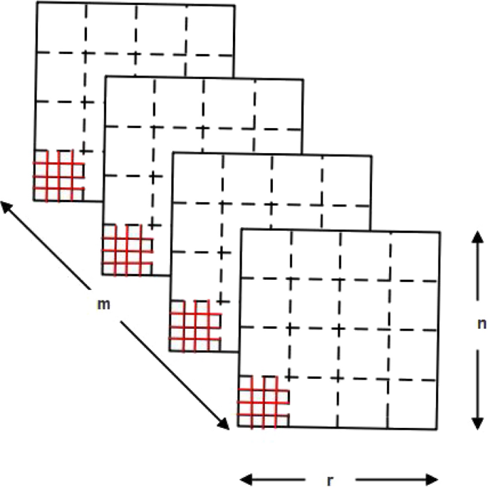

  

  Block multiplication scheming

  Parallelism is performed at various levels; each matrix multiplication is accelerated by parallelizing each block which in turn increases the system throughput. Several matrices or blocks multiples abruptly on the same chip decreasing the utilization of memory. The three block sizes in matrices X, Y, Z are calculated as three dimensions of parallelism, as parallelism is achieved as individual. Parallelizing over ‘n’ includes operating on rows of matrices X and Z one by one in parallel. Parallelizing over ‘r’ includes operating on columns of matrices Y and Z independently in parallel. Parallelizing over ‘m’ includes running columns of ‘X’ matrix with row of matrix ‘Y’, and matrix Z in standalone.

  To achieve parallelism along each dimension the block data allots uniform dimension over various processing units. If u1, u2 and u3 are blocks with dimension n, m and r respectively, then the parallelism p = u1u2u3. Each block of matrix X is partitioned along the dimension n/u1 × m /u2 resulting in u1u2 partition. Similarly block of matrix Y is partitioned along the dimension m/ u2 × r /u3 resulting in u2u3 partition and u1u3 partitions of dimension n/u1 × r /u3 for block of matrix Z. Each partition of X and Y block is linked to ‘u3’ and ‘u1’ multiply add units respectively. For the Z block, the partition is obtained by adding outputs of ‘u2’tomultiply add unit.

• (ii) Scheduling

  Scheduling denotes the way in which the multiplication and addition operations are performed. Matrix multiplication involves nmr multiplication and addition. In a single time slot, when a schedule assigns multiple arithmetic operations, it is a parallel schedule. In linear algebra three vector operations such as inner product, the middle product and the outer product are used to implement matrix multiplication. The proposed work processes the outer product which is obtained by multiplying the column element of matrix X by the row element of matrix Y. Each outer product of a column element and a row element produces the final value of the entire Z matrix. In two ways the outer product schedule are implemented. In the first case, the column major matrix X elements are reused and to produce a complete layer of matrix Z by multiplying each elements of a given column by the same row of matrix Y. In the second case, matrix Y elements are reused in a row major order, where every given row elements are multiplied by the similar column matrix X elements to produce a final value of matrix Z. In both the cases, the schedule reuses the column of matrix X elements, row of matrix Y elements and entire matrix Z elements.

  In matrix multiplication, column and row element multiplications are independent but addition depends on multiplication and other addition process, the update form of matrix multiplication is given below.

  $${z}_{ij}= \sum_{k=1}^{M}{x}_{ik}. {y}_{kj}+{z}_{ij}$$

  (10)

  Computing an element z_ij of matrix Z requires adding M products to the initial value of z_ij. Accumulating the sum of M + 1 numbers involves M interdependent additions. In pipelining operations, Read After Write (RAW) data hazards occur when using the same pipelined adder to accomplish two inter dependent additions i.e., the value is read earlier it has been written. To prevent data hazards the inter-dependent tasks must be separated by more clock cycles. In matrix multiplication, add-after-multiply and add-after-add are the two data dependencies. By enforcing the following measure the data hazards can be prevented.

  (i) Create a long multiply add pipeline by performing addition after the multiplication.

  (ii) Ensure that at appropriate cycle, when the product reaches the adder, the second operand to addition is provided.

  The above measures confirm that the two operations are provided with enough clock cycles for the first operation of multiplication to complete, thus avoids data hazard.

• (iii) Block size

  Three parameters that define the block size are n, m, and r. For larger blocks, during each compute phase it takes longer time to transfer. Moreover, the number of computation in compute phase is also affected by the shape of the blocks, which may be square or rectangle. For a matrix multiplication computation, the number of multiply add operations is given by

  $${\text{Number of multiply add operations}} = nmr$$

  (11)

  Block dimensions can be optimized to reduce the data transfer time by reducing the transfer rate. The optimizations result in the following constraints.

  $$nm + mr + nr \le S$$

  (12)

  wheren ≥ 1, m ≥ 1, r ≥ 1 andS be the used on-chip memory.

  Each compute phase execute one block multiplication, which include nmr scalar multiplication and additions. Thus, the function to maximize the number of multiply add operations per compute phase is given by

  $${\text{f}}\left( {n, \, m, \, r} \right) = nmr$$

  (13)

  If the blocks are of equal size, maximizing the function f result in

  $$n=m=r=\sqrt{\frac{S}{3}}$$

  (14)

  The total number of elements transfer for reusing block of matrix X is given by

  $${f}_{X}\left(n,m,r\right)=NM+\frac{NMR}{n}+\frac{2NMR}{m}$$

  (15)

  The first term, NM represents the number of transfer for matrix X. Each block is transferred and reused exactly once. So the amount of elements is equal to the amount of data transfer. The number of transfer for matrix Y elements is given in the second term. A block of matrix Y has mr elements. There are R/r × M/m blocks in matrix Y. Each block is transferred and multiplied N/n times in a column of matrix X. Hence the number of transfers of matrix Y elements is

  $$mr \times \frac{R}{r}\times \frac{M}{m}\times \frac{N}{n}= \frac{NMR}{n}$$

  (16)

  The third term in Eq. (13) is the number of transfer of matrix Y elements. A block of matrix Z has nr elements and N/n × R/r blocks. Each block is transferred twice and updated M/m times. Hence the number of transfers of matrix Y elements is

  $$nr \times \frac{N}{n}\times \frac{R}{r}\times \frac{M}{m}\times 2= \frac{2NMR}{m}$$

  (17)

  The total number of elements transfer for reusing block of matrix Y is given by

  $${f}_{Y}\left(n,m,r\right)=\frac{NMR}{r}+ MR+\frac{2NMR}{m}$$

  (18)

  The first term, represents the number of transfer for matrix X elements. Each block is transferred and multiplied R/r times in a row of matrix Y. There are nm elements in a block of matrix X and there are N/n × M/m blocks. The number of transfer for matrix X elements is

  $$nm \times \frac{N}{n}\times \frac{M}{m}\times \frac{R}{r}= \frac{NMR}{r}$$

  (19)

  The second term in Eq. (16) represents the number of transfer for matrix Y elements. Each block is transferred and reused exactly once. So the number of elements transfer is equal to the number of elements in the matrix Y. The third term in Eq. (16) is the number of transfer of matrix Z elements. When blocks of either of matrices X or Y are reused the number of elements transfer is same.

  The total number of elements transfer for reusing block of matrix Z is given by

  $${f}_{Z}\left(n,m,r\right)=\frac{NMR}{r}+\frac{NMR}{n}+2NR$$

  (20)

  The first term, represents that NM elements of matrix X is transferred R/r times, whereas for the second term in Eq. (18) each of the MR elements of matrix Y is transferred N/n times. Each element of matrix Z is transferred twice which is shown as third term.

• (iv) Double buffering

  Double buffering means assigning enough storage for two blocks of each matrix, for the purpose of permitting the data fetch stage and compute stage to execute overlapping. The overlapping operation reduces the total computation time. With double buffering, the compute phase starts when the first block of each matrix is transferred into the buffer. While the compute stage is processing the first buffer, the fetch phase starts replacing the content of second buffers. For all block multiplication, the total compute time in cycles is given by

  $${T}_{Compute}=\frac{NMR}{P}$$

  (21)

  where P is the number of multiply add units. For example, multiplying block size of 256 × 256 using 40 multiply add unit takes 419,430 cycles.

3 Result and discussion

The proposed block matrix multiplication using Strassen and Urdhva Tiryagbhyam multiplier is experimented using Xilinx 13.5 simulating tool and implemented in virtex-5 xc5vsx240t FPGA. The matrix multiplication algorithm exploits parallelism at various levels and by proper scheduling matrix elements are reused. Figure 4 shows the compute cycle vs matrix size. As the matrix size increases, the computation time also increases. The number of processing element performs arithmetic operations can be used to calculate the time spent in the computation cycle. Each PE produces a new output in every clock cycle.

Fig. 4

Compute time vs matrix size

Figure 5, shows the operating frequency vs number of PEs. As the number of PEs increases, the frequency decreases.The performance of the architecture depends on the speed of the processing element. The parallelization strategy allows the use of many processing elements in parallel. Each PEs consist of an arithmetic units which contains a floating point UrdhvaTiryagbhyam multiplier and an adder. The data in the sub blocks are transferred to the PEs internal buffer and the results are stored in the output buffers.

Fig. 5

Operating frequency vs. number of PEs

Figure 6 shows the performance vs. number of PEs. The performance of the architecture increases linearly with the processing elements. For floating point computation, the performance is measured in terms of number of floating point computation performed per second, designated as FLOPS (Floating Point Operations).

Fig. 6

Performance vs. number of PEs

Table 2 compares the performance of multiplier unit. The overall performance of the architecture is based on the performance of the multiplier units. When compared with (Dou et al. 2005) and (Zhang et al. 2013) the proposed multiplier unit occupies less area and the delay is also reduced when compared with Arish and Sharma (2016).

Table 2 Performance analysis of block matrix multiplication

Table 3 compares the performance of block matrix multiplication in terms of PEs, frequency and FLOPS. The proposed architecture achieves peak performance of 20.6 GFLOPS with 40 PEs operating at 265 MHz which is better when compared with Khayyat and Manjikian (2014) and Dou et al. (2005). Table 4 shows the performance measures for multiplier units. The area and delay of the proposed multiplier is less compared to the work of Arish and Sharma (2016).

Table 3 Comparison of the performance measures for block matrix multiplication

Table 4 Performance measures for multiplier units

Table 5 shows the analysis of the block dimension with performance time. The number of clock cycles used in the computation phase is known as compute time and the number of cycles spent in the data transfer phase is transfer time. Total time for computation is determined from two mechanisms: data computation time and transfer time. From Table 5 it is observed that the transfer time is 25% less than the computation time. Table 6 shows the block dimension vs size of on chip memory. As the block dimension increases the size of on chip memory also increased.

Table 5 Block dimension vs performance time

Table 6 Block dimension vs size of memory

Figure 7 shows the Comparison of parameter measures between the proposed and existing methods for block matrix multiplication. The simulation result of block multiplication using Strassen and Urdhva Tiryagbhyam multiplier is shown in Fig. 8. The input matrix is subdivided into sub matrices of size 2 × 2 and after multiplication the results are stored in registers. FPGA implementation uses LUT instead of memory element in ASIC implementation to store the results. Based on divide and conquer method, the input matrix A and B is subdivided into sub matrices of size 2 × 2 ie. a11[63:0], a12[63:0], a21[63:0], a22[63:0], a11[63:0], a12[63:0], a21[63:0], a22[63:0] and after multiplication the results are stored in registers t1(63:0), t2(63:0), t3(63:0) and t4(63:0).

Fig. 7

Comparison of parameter measures between the proposed and existing methods for block matrix multiplication

Fig. 8

Wave form of the proposed Strassen matrix multiplication

Figure 9 shows the Register Transfer Level schematic of the proposed architecture. It is generated after the synthesis process. It shows a representation of the pre-optimized design in terms of generic symbols such as adders, multipliers, counters, AND gates and OR gates. Figure 10 shows the technology schematic of the proposed architecture.

Fig. 9

RTL schematic of the proposed Strassen based method

Fig. 10

Technology schematic of the proposed method

4 Conclusion

The architecture performs block multiplication and the multiplication is parallelized employing several arithmetic units. Subsequently, the computation and the memory operation are also parallelized to perform the operations simultaneously. Further, the scheduling assigns multiple arithmetic operations in a single time slot in order for the data reuse to increase the system efficiency. Also in addition, the proposed architecture implements double buffering in two on-chip memory blocks for each matrix to overlap the transfer phase and the compute phase. The performance of the block matrix multiplication is 20.6 GFLOPS with 40 processing elements at a frequency of 265.31 MHz. The delay for the proposed architecture is 12.576 ns.

References

Amrutha, K., Ravi Kumar, M.N., Panduranga, H.T.: Implementation of dense matrix multiplication. In: Proceedings of 2nd ASAR International Conference, pp. 17–20 (2015)
Arish, S., Sharma, R.K.: Run time reconfigurable multi precision floating point matrix multiplier intellectual property core on FPGA. Circuits Syst. Signal Process. 36(3), 998–1026 (2016)
Cannon, L.E.: A cellular computer to implement the kalman filter algorithm. PhD dissertation. Montana State University (1969)
Chetan, S., Sourabh, K.S., Lekshmi, V., Sudhakar, S., Manikandan, J.: Design and evaluation of floating point matrix operations for FPGA based system design. Procedia Comput. Sci. 171, 959–968 (2020)
Choi, J.: A new parallel matrix multiplication algorithm on distributed-memory concurrent computers. Concurr. Pract. Exp. 10(8), 224–229 (1997)
Choi, J., Dangarra, J.J., Pozo, R., Walker, D.W.: PUMMA: parallel universal matrix multiplication algorithms on distributed memory concurrent computers. Concurr. Pract. Exp. 6(7), 543–570 (1994)
Dou, Y., Vassiliadis, S., Kuzmanov, G.K., Gaydadjiev, G.N.: 64-bit floating point FPGA matrix multiplication. In: Proceeding of the ACM/SIGDA 13th International Symposium on Field Programmable Gate Arrays (FPGA). pp. 86–95 (2005)
Fox, G.C., Otto, S.W.: Matrix algorithms on a hypercube I: matrix multiplication. Parallel Comput. 4(1), 17–31 (1987)
Geijn, R.A.V., Watts, J.: SUMMA: scalable universal matrix multiplication algorithm. Concurr. Pract. Exp. 9(4), 255–274 (1998)
Jagadguru Swami Sri BharatiKrsnaTirthaji Maharaja.: Vedic mathematics or sixteen simple mathematical formulae from the Vedas. MotilalBanarsidass, Delhi (1985)
Kalaiselvi, A.: Multimedia security for image encryption using transformation matrix. Maejo Int. J. Sci. Technol. 1(3), 79–88 (2010)
Kang, B.-H.: A review on image and video processing. Int. J. Multimed. Ubiquitous Eng. 2(2), 49–64 (2007)
Khayyat, A., Manjikian, N.: Analysis of blocking and scheduling for FPGA based floating point matrix multiplication. Can. J. Electr. Comput. Eng. 37(2), 65–75 (2014)
Kumar, V.B.Y., Joshi, S., Patkar, S.B., Narayanan, H.: FPGA based high performance double precision matrix multiplication. Int. J. Parallel Prog. 38(3), 322–338 (2010)
Li, K.: Constant time boolean matrix multiplication on a linear array with a reconfigurable pipelined bus system. J. Supercomput. 11(4), 391–403 (1997)
Li, K., Pan, V.Y.: Parallel matrix multiplication on a linear array with a reconfigurable pipelined bus system. IEEE Trans. Comput. 50(5), 519–525 (2001)
Matam, K.K., Prasanna, V.K.: Energy efficient large scale matrix multiplication on FPGAs. In: Proceedings of the International Conference on Reconfigurable Computing and FPGAs (ReConFig). pp. 1–8 (2013)
Matam, K.K., Le, H., Prasanna, V.K.: Evaluating energy efficiency of floating point matrix multiplication on FPGAs. In: Proceeding of the IEEE High Performance Extreme Computing Conference (HPEC). pp. 1–6 (2013)
Palacios, I., Medina, M., Moreno, J.: Matrix multiplication on digital signal processors and hierarchical memory systems. In: Baeza-Yates, R., Manber, U. (eds.) Computer Science, pp. 473–483. Springer, Boston, MA (1992)
Pan, V.: Complexity of parallel matrix computation. Theoret. Comput. Sci. 54, 65–85 (1987)
Pan, Y., Li, K., Zheng, S.Q.: Fast nearest neighbor algorithms on a linear array with a reconfigurable pipelined bus system. Parallel Algorithms Appl. 13(1), 1–25 (2007)
Pedram, A., Geijin, R.A., Gerstlauer, A.: Co-design tradeoffs for high-performance low power linear algebra architectures. IEEE Trans. Comput. 61(12), 1724–1736 (2012)
Prabhune, O., Sabale, P., Sonawane, D.N., Prabhune C.L.: Image Processing and Matrices. In: International conference on Data Management Analytics and Innovation (ICDMAI). pp. 166–171 (2017)
Qasim, S.M., Abbasi, S.A., Almashary, B.: FPGA-based design and realization of fixed and floating point matrix multipliers: a review. J. Active Passiv. Electron. Devices 5, 181–189 (2010)
Sajish, C., Abhyankar, Y., Ghotgalkar, S., Venkates, K.A.: Floating point matrix multiplication on a reconfigurable computing system. In: Current Trends in High Performance Computing and its Applications, pp. 113–122. Springer, Berlin (2005)
Shen, H., Chen, J.: Efficient matrix multiplication on wireless sensor networks. In: Proc of 7th International Conference on Grid and Cooperative Computing: 331–341 (2008)
Silva, H.D., Gustafson, J.L., Wong, W.F.: Making Strassen matrix multiplication safe. In: Proceedings of the 25th International Conference on High Performance Computing, pp. 173–182 (2018)
Singh, K.N., Tarunkumar, H.: A review on various multipliers designs in VLSI. In: Annual IEEE India Conference (INDICON), pp. 1–4 (2015)
Sonawane, D.N., Sutaone, M.S., InayatMalek: Resource efficient 64-bit floating point matrix multiplication algorithm using FPGA. In: IEEE Region 10 Conference TENCON, pp. 1–5 (2009)
Stojcev, M.K., Milovanovic, I.Z., Radonjic, Z.C.: Some shifting methods for matrix multiplication. IEE Proc. E-Comput. Digital Tech. 132(1), 33–44 (1985)
Strassen, V.: Gaussian elimination is not optimal. Numerischemathematik 13(4), 354–356 (1969)
Thabet, K., Al-Ghuribi, S.: Matrix multiplication algorithms. Int. J. Comput. Sci. Netw. Secur. 12(2), 74–79 (2012)
Tiwari, S., Singh, S., Meena, N.: FPGA design and implementation of matrix multiplication architecture by PPI-MO techniques. Int. J. Comput. Appl. 80(1), 19–22 (2013)
Van De Geijn, R.A., Watts, J.: SUMMA: scalable universal matrix multiplication algorithm. Concurr.: Pract. Exp. 9(4), 255–274 (1998)
Zhang, T., Li, C.T., Qin, Y., Nie, M.: An optimized floating point matrix multiplication on FPGA. Inf. Technol. J. 12(9), 1832–1838 (2013)
Zhou, L., Prassana, V.K.: High performance designs for linear algebra operations on reconfigurable hardware. IEEE Trans. Comput. 57(8), 1057–1071 (2008)
Acknowledgements
This research has been funded by the research general direction at Universidad Santiago de Cali, Colombia under call no 01-2022. This research is collaborated with the authors in these institutions such as St. Xavier’s Catholic College of Engineering, Tamilnadu, India, Gems Educational Institutions, Sbte, Karunya Institute of Technology and Sciences, Coimbatore, India, and Al-nahrain university, al-nahrain nonrenewable energy research center Baghdad, Iraq.
Author information
Authors and Affiliations
Corresponding author
Rights and permissions
Springer Nature or its licensor (e.g. a society or other partner) holds exclusive rights to this article under a publishing agreement with the author(s) or other rightsholder(s); author self-archiving of the accepted manuscript version of this article is solely governed by the terms of such publishing agreement and applicable law.
About this article
Cite this article
Bessant, Y.R.A., Jency, J.G., Sagayam, K.M. et al. Improved parallel matrix multiplication using Strassen and Urdhvatiryagbhyam method. CCF Trans. HPC 5, 102–115 (2023). https://doi.org/10.1007/s42514-023-00149-9
Received:
Accepted:
Published:
Issue Date:
DOI: https://doi.org/10.1007/s42514-023-00149-9