A novel semi supervised approach for text classification

Abstract

Text categorization, also known as text classification is a supervised classification problem. It aims to assign a predefined class label or group to a new or unknown text document. Most of the time we need a collection of large data from each class to train the classifier. It may be noted that, it is very hard or expensive to collect labelled text data. In most cases we assign the label manually which is neither cost effective nor efficient. In this paper, we have introduced a semi-supervised classification approach where the learner needs very small amount of labelled data with a large amount of unlabeled data to assign a class label to a new or unknown text document. The proposed method uses Kohonen self organizing map (SOM) for labelling the unlabeled data and three classifiers namely support vector machine (SVM), Naïve Bayes (NB), and decision tree (DT): classification and regression tree (CART) for observing the accuracy of classification. The experimental results obtained show the effectiveness of our proposed method.

1 Introduction

Advancement of social networking, blogging, micro-blogging has provided the opportunity to develop various applications in natural language processing (NLP). Text classification is a very popular research area of NLP. Over the last decade it grew exponentially [1,2,3,4,5,6] due to easy accessibility of the digital text documents. Text classification implies automated assignment of textual data to predefined classes. Sometimes either the number of such classes is not known or the class labels are not known. In this case initially some clustering technique is employed to obtain the appropriate grouping of a given set of text documents, then such groups are labelled based on some criteria or heuristic.

Several machine learning algorithms had been applied successfully to categorize text documents based on their content. Perhaps Naive Bayes (NB) algorithm is the frequently used classifier to solve text categorization problem. Researchers used two different generative models: multi-variate Bernoulli [7,8,9,10,11] and multinomial [12,13,14,15,16] event model while designing the NB classifier. Algorithms based on artificial neural network (ANN) [17,18,19], decision tree (DT) [20,21,22,23], k-nearest neighbor (KNN) [24,25,26,27], and SVM [28, 29] had been employed frequently to solve the text categorization problem. Ruiz and Srinivasan [5] proposed a method based on principal component analysis (PCA) and class profile based features (CPBF). It requires the number of classes present in the set of text documents to be known a priori. Text classification methods using linear vector quantizer (LVQ) network also require the number of classes to be supplied. A web news classification technique using neural networks proposed by Selamat et al. [6], which is based on PCA and requires the class profile-based features to be known a priori. Supervised text classification algorithms need a collection of sufficient number text data from each of the classes to predict. Classifiers performance varies with the nature of the dataset. So, we need a dataset that is not only large but also well distributed over the range of the classes. But labelled text data is hard to find/expensive. Most of the time we do the class labelling task manually which is neither efficient nor cost effective. Using clustering algorithms, we can extract some groups from a dataset when the class label is absent or not available. Text clustering is another popular research area in Text domain. Details of the several text clustering algorithms can be found in [30,31,32,33,34,35,36,37,38]. Clustering may find the correct groups presented in a collection of text, but it cannot provide the context or class label of the groups.

In this paper we have proposed a semi-supervised approach to predict a class label for new text document. In this approach we need only few labelled text data and large number of unlabeled data to do the prediction. Our proposed method uses Kohonen SOM and three classifiers SVM, NB, and DT (CART). We have extracted the groups present in the text data by applying Kohonen SOM. Then we took votes using the labelled data to assign class label to our extracted groups. In other words, we find the class label for which the number of labelled data present in that group is larger than that for all the remaining class label. This method is used to label all the groups of the text documents generated by SOM. In this way we are able to generate a complete labelled dataset from a dataset which is mostly unlabeled as stated earlier. The newly labeled data are used to train three classifiers namely SVM, NB, and DT (CART) and previously labelled data are used for the testing purpose. It may be noted that the results obtained with the aforesaid three most widely used classifiers are satisfactory.

The basic sketch of this paper is as follows. Next section presents the statement of the problem. Section 3 thoroughly describes the proposed method. Experimental results are presented in Sect. 4. Concluding remarks can be found in Sect. 5.

2 Statement of the Problem

Given a set of text documents $D = \{ d_{1} , d_{2} , \ldots d_{i} , \ldots d_{n} \}$, where $i_{th}$ document $d_{i}$ is represented by its pattern vector $x_{i}$ and $n$ is the number of documents. Let the set of pattern vectors $S = \left\{ {x_{1} ,x_{2} , \ldots x_{i} , \ldots x_{n} } \right\} \subseteq {\mathbb{R}}^{m}$, where $m$ is the dimensionality of the feature space. The value of $m$ is decided in the Step 5 of feature selection steps described below. The problem is to assign each text document $d_{i}$ into one of the predefined categories or labels $\left( {l_{i} } \right)$. Let the set of categories is $L = \left\{ {l_{1} , l_{2} , \ldots l_{i} , \ldots , l_{p} } \right\},$ where $p$ is the number of class labels such that $p \ll n$. A typical text or document categorization task assigns a boolean value to each pair $\langle x_{i} , l_{j}\rangle \in D \times L$. A $True$ value is assigned to $\langle x_{i} , l_{j}\rangle$ when a decision has been made to assign a label $l_{j}$ to a document $x_{i}$ otherwise a $False$ value is assigned. Let a subset $D_{l} \subseteq D,$ consists of labelled text documents and $D_{ul} \subseteq D$ consists of unlabelled text documents, where $\left| {D_{l} } \right| \ll \left| {D_{ul} } \right|, D_{l} \mathop \cup \nolimits D_{ul} \equiv D$ and $D_{l} \mathop \cap \nolimits D_{ul} \equiv \emptyset$. So our problem is to assign boolean values to the pairs $\langle x_{i} , l_{j}\rangle \in D_{ul} \times L$.

According to Bag-of-words technique, we can represent a text document $(x_{i} )$ as a vector of frequency count of the words present in the text document. Essentially, the dimension of such a vector will be very high if we consider all the words. We have applied the following steps to remove some insignificant words that leads to dimensionality reduction of the feature vectors.

Step 1::

Remove stop words from the documents: Remove stop words like determiners (e.g. a, an, the etc.), conjunctions (e.g. and, or, but etc.), prepositions (e.g. across, after, behind etc.), some adverbs (e.g. here, there, out etc.) from all the text documents. Complete list of the stop words can be found in [39].

Step 2::

Extraction of the root words: Use ‘Porter stemmer’ to remove morphological affixes from the words.

Step 3::

Select only the unique words from the documents. Suppose we have two documents $d_{1}$ and $d_{2}$, where $d_{1} = \left\{ {w_{1} , w_{2} , w_{1} ,w_{3} ,w_{4} } \right\}, d_{2} = \left\{ {w_{1} , w_{2} , w_{3} ,w_{4} ,w_{3} , w_{5} ,w_{6} } \right\}$, so the set of unique words is $W_{p} , W_{p} = \{ w_{1} , w_{2} , w_{3} ,w_{4} ,w_{5} ,w_{6} \} .$

Step 4::

Define $EF_{{wl_{k} }}$ to be the elimination factor for the word $w$ in context $l_{k}$ as follows: $EF_{{wl_{k} }} = \frac{{n_{{l_{k} }} }}{N}$, where $n_{{l_{k} }}$ is the frequency count of the word in the context $l_{k}$ and $N$ is the total frequency count.

Remove all the words that have $EF_{{wl_{k} }}$ value less than a predefined threshold $( 0.9)$ from $W_{p}$ [41].

Let $W_{ef}$ denotes a set of words that are having $EF_{{wl_{k} }}$ value less than the predefined threshold. So $W_{q} = W_{p} - W_{ef} = \{ w_{i} :w_{i} \in W_{p} \;and\; w_{i} \notin W_{ef} \}$. We have observed that $\left| {W_{q} } \right| \ll \left| {W_{p} } \right|.$

Step 5::

All the remaining words in $W_{q}$ are selected as the features of the text documents. Note that the feature values are finite positive integers (i.e. $n_{{l_{k} }}$) in nature.

Step 6::

Construct pattern vectors for each of the document using the features selected in Step 4 and the length of the pattern vector is $\left| {W_{q} } \right|.$

Please note that using Step 4, we can remove those words that are used frequently irrespective of the class labels or context. For example, the word “win” can occur frequently in all the news article category (i.e. Sports, Travel, Business, and Entertainment) considered for the experimentation. Thus, the word “win” will have lower value of $w_{{efl_{j} }}$. It may also be noted that although the parameter ‘$tf - idf$’ value is useful for estimating the relative importance of a specific word in terms of its total number of occurrence in the whole corpus but it does not at all reflect its importance for detection of a specific context/class.

We need to design a system which can assign a class level to a new or unlabelled text document.

3 Proposed method

In this work we have proposed a semi supervised approach to predict the class label of new or unlabelled text documents. Our proposed method uses Kohonen SOM and SVM algorithm. Kohonen SOM is used to discover the groups present in a given set of text documents. SVM is used to assign class labels to unlabelled text documents. Following algorithm presents the method for grouping the text documents.

We have manually labelled a small portion $(D_{labelled} )$ of a given dataset ($D$). By taking about 50% of the labelled data, a test dataset $D_{test}$ has been constructed. Rest of the labelled data, $D_{koho - labelled} ,( D_{koho - labelled} = D_{labelled} - D_{test} )$ will be used to label unknown data. It may be noted that, the test dataset ($D_{test}$) is used only for the testing purpose. We have applied Kohonen SOM algorithm on the Dataset $D_{input}$,$(D_{input} = D - D_{test} )$ to extract the groups. In other words, the unlabeled data and 50% of the manually labelled data are used in this process. Extracted groups are labeled by majority voting with the help of labeled data ($D_{koho - labelled}$). We have used only the newly labelled data $(D_{train} = D_{input} - D_{koho - labelled} )$ to train our classifiers. The part of the manually labelled data $(D_{test} )$ initially kept aside to act as a test dataset are now being used to test the performance of the chosen classifiers.

Following algorithm describes the proposed method for labelling the unknown data.

3.1 Algorithm: to assign label to a set of unlabeled text documents

For each text document $d_{i}$ of a set of text documents $D_{input} = \{ d_{1} ,d_{2} , \ldots d_{i} , \ldots d_{n} \}$, apply its pattern vector $x_{i}$ to the Kohonen’s network. Here the Kohonen network will have $m$ number of input nodes (since $m$ is the dimensionality of the feature space) and $k (k = 16)$ output nodes. Output nodes are arranged in a 2-dimensional $4 \times 4$ grid. After convergence of the Kohonen’s Algorithm, each high-density region of the feature space will be represented by one or more output nodes of Kohonen networks.

Input:

• Set of pattern vectors $S, S = \left\{ {x_{1} ,x_{2} ,..x_{i} ,..x_{n} } \right\} \subseteq {\mathbb{R}}^{m}$, where $n = |D_{input} |$ and $m$ is the dimensionality of the feature space.

Output:

• A labelled set ($D_{input} - D_{koho - labelled}$) of text documents which were previously unlabeled.

Steps:

• 1. Initialize the weight $W_{j} , W_{j} \in {\mathbb{R}}^{m}$ from $m$ inputs to the $k$ output nodes to small random values.

• 2. Present a new input.

• 3. Compute distance to all output nodes

  $$dist_{j} = \mathop \sum \limits_{i = 1}^{n} (x_{i} \left( t \right) - w_{ij} (t))^{2} .$$

• 4. Select the kohonen-output node $(j^{*} )$ with minimum distance.

• 5. Update weight to node $(j^{*} )$.

  $$W_{ij} \left( {t + 1} \right) = W_{ij} \left( t \right) + \beta \left( t \right)\left( {x_{i} \left( t \right) - w_{ij} \left( t \right)} \right), where \;0 < \beta \left( t \right) < 1.$$

• 6. Repeat by going step 2. (Until all the inputs are presented).

• 7. Repeat by going step 3 (Until $t = max\_itn$).

• 8. Construct a Minimum Spanning Tree $S_{op} (V, E_{s} )$, where $V$ is the set of output nodes ($V \equiv J = \left\{ {j_{1} , j_{2} , \ldots j_{i} , \ldots j_{k} } \right\}$) and $E_{s} \subset E, E = \parallel j_{u} ,j_{v}\parallel , 1 \le u \le k\; and\; 1 \le v \le k.$

• 9. Compute $e_{mean} = \frac{{\mathop \sum \nolimits_{i = 1}^{n} e_{i} }}{n}, \;where \;e_{i} \in E_{s}$.

• 10. Compute the number of clusters $(q)$ present from $S_{op}$: $q = \left| {E_{s}^{'} \left( {where\, e\, \in E_{s}^{'} \,and\, e_{i} > c*e_{mean} } \right)} \right| + 1,$ where $E_{s}^{'} \in E_{s}$ and $c$ is a real constant.

• 11. Divide the $k \left( {k = \left| V \right|} \right)$ number of nodes into $q$ number of clusters $\left( {C_{1} , C_{2} , \ldots C_{i} , \ldots C_{q} } \right)$ by disconnecting the edges $e_{i} > c*e_{mean} ,$ where $c$ is a real constant. We need to have $p = q$. If $p < q$ increase the value of $c$ in steps of $0.1$ until we get $p = q$ else if $p > q$ decrease the value of $c$ in steps of $0.1$ until we get $p = q$.

• 12. Assign each $d_{i}$ of $D_{input}$ to the cluster $C_{y}$ if the kohonen node which is nearest to $d_{i}$ belongs to cluster $C_{y}$.

  $$d_{i} \in C_{y}\quad \textrm{if}\quad \parallel d_{i} - j_{y}\parallel^{2} < \parallel d_{i} - j_{z}\parallel^{2} \forall y,z \in \left\{ {1,2, \ldots ,k} \right\}, y \ne z \;\textrm{and}\;j_{y} \in C_{y} .$$

• 13. Assign class label $l$ to $i_{th}$ cluster $C_{i}$ based on voting of class labels of manually labelled members present in $C_{i}$.

  $C_{i} = \left\{ {l:\# n_{l} > \# n_{r} } \right\}\forall l,r \in \left\{ {1,2,..,p} \right\} \quad \textrm{and}\quad l \ne r$, where $\# n_{l} \;\textrm{and}\; \# n_{r}$ denotes the number of instances with the class label $l$ and $r$ respectively in cluster $C_{i}$ and $p$ is the number of class labels.

• 14. Return a labelled set ($D_{input} - D_{koho - labelled}$) of text documents which were previously unlabeled.

To validate the class label assignment, we can use any exiting classifier. We have chosen three very popular and widely used classification algorithms—Naïve Bayes (NB), decision tree (DT): classification and regression tree (CART), and support vector machine (SVM). We have trained these classifiers with the dataset $D_{train}$ (training dataset) and tested the classifiers with the dataset $D_{test}$ (test dataset). In this experiment we have used 10-fold cross validation approach.

3.2 Naïve Bayes

Assume we have a training dataset $D$, given as $\{ \left( {X_{1} , y_{1} } \right), \left( {X_{2} , y_{2} } \right), \ldots ,\left( {X_{i} , y_{p} } \right), \ldots ,\left( {X_{\left| D \right|} , y_{q} } \right)\}$ where $X_{i}$ is the set of training tuples or feature vector with class label $y_{p}$ and $X_{i} = \vec{X} = \{ x_{1} ,x_{2} , \ldots ,x_{n} \}$. Now, NB predicts the class label $y_{q}$ for any $\vec{X}$ according to the following probability.

$$p\left( {y_{q} |\vec{X}} \right) = p\left( {y_{q} |x_{1} ,x_{2} , \ldots ,x_{n} } \right)\;{\text{for}}\; q = 1, \ldots ,r$$

(1)

According to the Bayes’s theorem, we can write,

$$p\left( {y_{q} |\vec{X}} \right) = \frac{{p\left( {\vec{X} |y_{q} } \right) \cdot p(y_{q} )}}{{p(\vec{X})}} = \frac{{p(x_{1} ,x_{2} , \ldots ,x_{n} |y_{q} ) \cdot p(y_{q} )}}{{p(x_{1} ,x_{2} , \ldots ,x_{n} )}}.$$

(2)

The denominator is not dependent on $y_{q}$ and the value of $\vec{X}$ is given so effectively it is a constant. So, we are interested only in the numerator. The factor $p(x_{1} ,x_{2} , \ldots ,x_{n} |y_{q} )$ in numerator can be written as following using chain rule.

$$p\left( {x_{1} ,x_{2} , \ldots ,x_{n} |y_{q} } \right) = p(x_{1} |x_{2} , \ldots ,x_{n} ,y_{q} ) p(x_{2} |x_{3} , \ldots ,x_{n} ,y_{q} ) \cdots p(x_{n - 1} |x_{n} ,y_{q} )p(x_{n} |y_{q} )$$

(3)

Now, if we assume that any feature $x_{i}$ is independent of any other feature $x_{j}$ given the class label $y_{q}$ then using Eq. (3) we can write

$$p\left( {x_{i} |x_{i + 1} , \ldots , x_{n} ,y_{q} } \right) = p\left( {x_{i} |y_{q} } \right) \Rightarrow p\left( {x_{1} , \ldots ,x_{n} |y_{q} } \right) = \mathop \prod \limits_{i = 1}^{n} p(x_{i} |y_{q} ).$$

(4)

So,

$$\begin{aligned} p\left( {y_{q} |x_{1} , \ldots ,x_{n} } \right) \propto p\left( {y_{q} ,x_{1} , \ldots ,x_{n} } \right) \hfill \\ \propto p\left( {y_{q} } \right) \cdot p(x_{1} , \ldots ,x_{n} |y_{q} ) \hfill \\ \propto p\left( {y_{q} } \right) \cdot \mathop \prod \limits_{i = 1}^{n} p(x_{i} |y_{q} ) \hfill \\ \end{aligned}$$

(5)

In practice, Binomial distribution or Gaussian distribution is used to model the class conditional feature probabilities $p(x_{i} |y_{q} )$. So we can assign a class label $y_{q}$ to a data $\vec{X}$ by computing $p\left( {y_{q} } \right) \cdot \mathop \prod \limits_{i = 1}^{n} p(x_{i} |y_{q} )$ for $q = 1, \ldots ,r$ and assigning $\vec{X}$ the class $y_{q}$ for which the value is largest. So we can write-

$$\bar{y} = \mathop {\text{argmax}}\limits_{{q \in \{ 1, \ldots ,r\} }} p\left( {y_{q} } \right) \cdot \mathop \prod \limits_{i = 1}^{n} p(x_{i} |y_{q} ),$$

where $\bar{y}$ is the predicted class label for $\vec{X}$.

3.3 Decision tree (CART)

CART algorithm recursively partitions a given training dataset ($D$) to obtain pure subsets with respect to a given class. A certain set of tuples $F (F \subseteq D)$ associated with each node of a tree can be splitted based on a specific test on an attribute. Suppose, we have a continuous attribute $C$, a threshold $t$, and the test is $C \le t$. We can do the partition on $F$ and generate two subsets (one for right branch and another one for left) based on the following criteria.

$$\begin{aligned} F_{r} = \{ f \in F:f\left( C \right) \le t\} \;{\text{and}} \hfill \\ F_{l} = \{ f \in F:f\left( C \right) > t\} \hfill \\ \end{aligned}$$

Similarly, the split can be done based on any categorical feature $H$. If, $H = \{ h_{1} ,h_{2} , \ldots , h_{k} \}$, then each branch $i$ can be constructed using the test $H = h_{i}$.

This recursive algorithm has a divide step to construct the decision tree by selecting the best split according to a predefined quality measure from all possible splits. Usually the algorithm evaluate each splits based on the impurity measurement. CART uses Gini index to measure the impurity. It may be noted that, the split should decrease the impurity of the parent node. Let the dataset has following scheme $(C_{1} , C_{2} , \ldots C_{i} ,\ldots,C_{m} ,Y)$, where $C_{i}$ is the attribute and $Y$ is the target class label. Let $(F_{1} , F_{2} , \ldots , F_{k} )$ be a split generated from a set of tuples $F$ and $IM()$ is the impurity measure function then the splitting criterion is

$$\Delta = IM\left( F \right) - \mathop \sum \limits_{i = 1}^{k} \frac{{\left| {F_{i} } \right|}}{\left| F \right|}IM(F_{i} )$$

(6)

For CART, $IM()$ is the Gini index.

$$IM\left( F \right) = Gini\left( F \right) = 1 - \mathop \sum \limits_{j = 1}^{n} q_{j}^{2}$$

(7)

where $n$ is the number of class and $q_{j}$ is the fraction of tuples in $F$ that belong to a particular class $y_{j}$.

$$q_{j} = \frac{{|\{ f \in F:f\left[ Y \right] = y_{j} \} |}}{|F|}$$

(8)

3.4 Support vector machine

Assume we have a training dataset $D$, given as $\{ \left( {X_{1} , y_{1} } \right), \left( {X_{2} , y_{2} } \right), \ldots ,\left( {X_{i} , y_{p} } \right) \ldots,\left( {X_{\left| D \right|} , y_{q} } \right)\}$ where $X_{i}$ is the set of training tuples or feature vector with class label $y_{p}$. It may be noted that $X_{i} \in {\mathbb{R}}^{n}$ and $y_{p} \in ( + 1, - 1)$. Given above stated situation, SVM [44, 45] requires solving the following minimization problem:

$$\begin{aligned} \mathop {\hbox{min} }\limits_{w, b, \xi } \frac{1}{2}w^{T} w + C\mathop \sum \limits_{i = 1}^{l} \xi_{i} , \hfill \\ {\text{subject to}}\; y_{p} \left( {w^{T} \emptyset \left( {X_{i} } \right) + b} \right) \ge 1 - \xi_{i} ,\;\xi_{i} \ge 0 \hfill \\ \end{aligned}$$

(9)

The function $\emptyset$ maps the feature vector $X_{i}$ to higher dimension space. In higher dimension SVM finds the hyperplane which separates the classes by maximum margin. $C$ is a penalty parameter and $C > 0$. We can define a kernel function $K\left( {X_{i} , X_{j} } \right) = \emptyset (X_{i} )^{T} \emptyset (X_{j} )$. Frequently used kernel functions are [46]:

• 1. Linear: $K\left( {X_{i} , X_{j} } \right) = X_{i}^{T} X_{j} .$

• 2. Polynomial: $K\left( {X_{i} , X_{j} } \right) = \left( {\gamma X_{i}^{T} X_{j} + r} \right)^{d} ,\gamma > 0.$

• 3. Radial basis function:

  $$K\left( {X_{i} , X_{j} } \right) = { \exp }( - \gamma\parallel X_{i} - X_{j}\parallel^{2} ),\gamma > 0.$$

• 4. Sigmoid:

  $$K\left( {X_{i} , X_{j} } \right) = \tanh (\gamma X_{i}^{T} X_{j} + r).$$

Here $\gamma , r,$ and $d$ are kernel parameters.

Linear kernel is best suited for linearly separable dataset. Polynomial, radial basis function, and sigmoid kernel functions are generally used on non-linearly separable dataset. These kernels are also known as non-liner kernels.

In our experiment, we have used linear kernel instead of non-linear kernels for following reasons:

• (i) Since text dataset is very high dimensional in nature, we can use linear kernel instead of nonlinear kernel without sacrificing any significant performance [46, 48].

• (ii) For linear kernel, there is no need for implicit mapping of data to high dimension $(\emptyset (X))$. So, training time for SVM with linear kernel is less than the SVM with nonlinear kernels.

• (iii) Unlike the non-liner kernels, we need to estimate only the penalty parameter $\left( C \right).$ Please note that, “grid search” have been used to find the optimum value of $C$. There exists several advanced methods (e.g. Randomized parameter optimization, Gradient based optimization, Bayesian optimization etc.) which can save computation cost. However, we prefer the simple “grid search” for following reasons.

  • (a) Since it is an exhaustive process it will return a good value.

  • (b) The computational time required to find a good value for only one parameter by “grid search” is not much than the time required for the above mentioned advanced techniques.

It may be noted that, in SVM ‘one vs. one’ approach is used over ‘one vs. all’ approach for two reasons. One is that, our problem deals with multiple classes. The other reason is that, training time required for ‘one vs. one’ approach is much less than ‘one vs. all’ approach [47].

4 Experimental results

We have tested our proposed technique on five different datasets from two different domains (i.e. News Articles and Product reviews).

Following are the news article datasets.

• 1. BBC Dataset [42]: This dataset contains 2225 news articles collected from BBC news website. Class labels are business (B), entertainment (E), politics (P), sport (S), and technology (T).

• 2. BBCSport Dataset [42]: This dataset contains 737 news articles collected from BBC Sport news website. Class labels are athletics (A), cricket (C), football (F), rugby (R), and tennis (T).

• 3. 20 Newsgroups_subset Dataset [43]: Original dataset contains 20,000 messages taken from 20 different newsgroups. 6000 messages are randomly chosen to form the subset. Multiple newsgroups are grouped together to form the class labels. Class labels are computer (C), sales (SA), politics (P), religion (R), science (SC), and sports (SP). Following Fig. 1 describes how class labels are formed.

  Fig. 1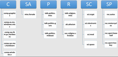

  

  Class description of the 20_newsgroup_subset dataset

To construct product review datasets, we have developed a web crawler and a page parser program. These programs will automatically collect consumer’s reviews on various products from a popular Indian e-Commerce site.

Following are the product review datasets.

• 1. Product Review 1: This dataset contains 4900 product reviews collected from Flipkart.¹ Class labels are camera (C), television (TV), mobile (M), and laptop (L).

• 2. Product Review 2: This dataset contains 3300 product reviews collected from Flipkart. Class labels are air conditioner (AC), refrigerator (R), tablet (T), and washing machine (WM).

Details of $D, D_{labelled} , D_{test} ,\quad \textrm{and}\quad D_{input}$ of five different experimental datasets can be found in Table 1. Detailed descriptions of five test datasets can be found in Tables 2, 3, 4, 5, and 6. Performance of NB classifier on the five experimental datasets can be found in Tables 7, 10, 13, 16, and 19. Tables 8, 11, 14, 17, and 20 describe the performance of DT (CART). Performance of SVM classifier can be found in Tables 9, 12, 15, 18, and 21. Comparisons among three different classifiers (i.e. NB, DT (CART), and SVM) can be found in Table 22.

Table 1 Description of experimental dataset

Table 2 Description of test data ($D_{test}$) for ‘BBC News’

Table 3 Description of test data ($D_{test}$) for ‘BBC Sport News’

Table 4 Description of test data ($D_{test}$) for ‘20 Newsgroups_subset’

Table 5 Description of test data ($D_{test}$) for ‘Product Review 1’

Table 6 Description of test data ($D_{test}$) for ‘Product Review 2’

Table 7 Confusion matrix for the classification results using NB classifier on BBC News Dataset

Table 8 Confusion matrix for the classification results using DT(CART) classifier on BBC News Dataset

Table 9 Confusion matrix for the classification results using SVM classifier on BBC News Dataset

Table 10 Confusion matrix for the classification results using NB classifier on BBC Sport News Dataset

Table 11 Confusion matrix for the classification results using DT (CART) classifier on BBC Sport News Dataset

Table 12 Confusion matrix for the classification results using SVM classifier on BBC Sport News Dataset

Table 13 Confusion matrix for the classification results using NB classifier on 20 News Groups_subset Dataset

Table 14 Confusion matrix for the classification results using DT (CART) classifier on 20 News Groups_subset Dataset

Table 15 Confusion matrix for the classification results using SVM classifier on 20 News Groups_subset Dataset

Table 16 Confusion matrix for the classification results using NB classifier on Product review 1 Dataset

Table 17 Confusion matrix for the classification results using DT (CART) classifier on Product review 1 Dataset

Table 18 Confusion matrix for the classification results using SVM classifier on Product review 1 Dataset

Table 19 Confusion matrix for the classification results using NB classifier on Product review 2 Dataset

Table 20 Confusion matrix for the classification results using DT (CART) classifier on Product review 2 Dataset

Table 21 Confusion matrix for the classification results using SVM classifier on Product review 2 Dataset

Table 22 Comparison of the classifiers

Overall accuracy of SVM, NB, and DT (CART) classifiers can be found in Table 22. We also have measured Kappa value to compare the performance of these three classifiers.

It can be noted from Table 22 that Kappa value is greater than 0.61 in every case. Kappa statistic or value represents the difference between accuracy of the classification system to the accuracy of a random system (e.g. Kappa of 0.7 means a classification system is 70% better than a random system). According to Landis and Koch [40] Kappa value of greater than 0.6 indicates a decent or significant classifier. Thus, we can conclude that our proposed method of labelling a large size of unlabeled data using a relatively small size of labelled data is efficient enough to provide an acceptable label of accuracy for classification.

We have reported our experimental results using labelled data ($D_{labelled}$) of size 10% of that of total dataset for first three datasets (i.e. BBC News Dataset, BBC Sport News Dataset, and 20 News groups_subset) in Table 22. It may be noted that these three datasets were already labelled. We have manually labelled 10% of that of total dataset ($D_{labelled}$) for last two datasets (i.e. Product Review 1, Product Review 2 Dataset). It may be noted that, these datasets were not labelled. We have also carried out experiment with different size of manually labelled data from 1 to 25% of the size of total dataset for two datasets (i.e. Product Review 1 and Product Review 2) to study the effect of size of manually labelled data on classification accuracy. Figures 2 and 3 present the findings of the said experiments.

Fig. 2

Change in overall accuracy w.r.t. percentage of labeled data (Product Review 1 dataset)

Fig. 3

Change in overall accuracy w.r.t. percentage of labeled data (Product Review 2 dataset)

The changes in overall accuracy w.r.t. initial number of labeled data in the total dataset, can be found in Figs. 2 and 3. As you can see from the Figs. 2 and 3, changes in the overall accuracies are very sharp when the number of labeled data is increasing from small but gradually it became stagnant with increment of the labeled data.

5 Conclusion

In this paper we have proposed a semi supervised method for text document classification. Note that, adequate number of labelled data required for training of classifiers are not always easily available. Here our intention is to use a small amount of labelled data to label a relatively large amount of unlabeled data. The proposed method uses Kohonen SOM for labelling the unlabeled data and three classifiers namely SVM, NB, and DT (CART) for observing the accuracy of classification. We have selected five datasets for experimentation. In all five datasets SVM delivers better performance than NB and DT (CART) classifiers. We have concluded that our proposed method can efficiently assign label to a set of large unlabeled data with the help of very small labelled dataset. In future, we will try to use various other clustering algorithms which can efficiently handle high-dimensional data to improve our system’s performance. Various feature selection techniques can be used to reduce dimensionality of the data.

References

Torkkola K (2004) Discriminative features for text document classification. Formal Pattern Anal Appl 6(4):301–308
Sebastiani F (2002) Machine learning in automated text categorization. ACM Comput Surv (CSUR). 34(1):1–47
Han EHS, Karypis G (2000) Centroid-based document classification: analysis and experimental results. In: European conference on principles of data mining and knowledge discovery. Springer, Berlin, pp 424–431
Basili R, Moschitti A (2001) A robust model for intelligent text classification. In: Proceedings of the 13th international conference on tools with artificial intelligence. IEEE, pp 265–272
Ruiz ME, Srinivasan P (1999) Hierarchical neural networks for text categorization (poster abstract). In: Proceedings of the 22nd annual international ACM SIGIR conference on research and development in information retrieval. ACM, pp 281–282
Selamat A, Yanagimoto H, Omatu S (2002) Web news classification using neural networks based on PCA. In: SICE 2002. Proceedings of the 41st SICE annual conference, vol 4. IEEE, pp 2389–2394
Robertson SE, Jones KS (1976) Relevance weighting of search terms. J Am Soc Inf Sci 27(3):129–146
Lewis DD (1992) An evaluation of phrasal and clustered representations on a text categorization task. In: Proceedings of the 15th annual international ACM SIGIR conference on research and development in information retrieval. ACM, pp 37–50
Kalt T, Croft WB (1996) A new probabilistic model of text classification and retrieval. Technical Report IR-78, University of Massachusetts Center for Intelligent Information Retrieval
Larkey LS, Croft WB (1996) Combining classifiers in text categorization. In: Proceedings of the 19th annual international ACM SIGIR conference on research and development in information retrieval. ACM, pp 289–297
Sahami M (1996) Learning limited dependence Bayesian classifiers. In: KDD, vol 96, pp 335–338
Lewis DD, Gale WA (1994) A sequential algorithm for training text classifiers. In: Proceedings of the 17th annual international ACM SIGIR conference on research and development in information retrieval. Springer, New York, pp 3–12
Guthrie L, Walker E, Guthrie J (1994) Document classification by machine: theory and practice. In: Proceedings of the 15th conference on computational linguistics. Association for Computational Linguistics, vol 2, pp 1059–1063
Li H, Yamanishi K (1997) Document classification using a finite mixture model. In: Proceedings of the 35th annual meeting of the association for computational linguistics and eighth conference of the European chapter of the association for computational linguistics, pp 39–47. Association for Computational Linguistics
Nigam K, McCallum A, Thrun S, Mitchell T (1998) Learning to classify text from labeled and unlabeled documents. In: Proceedings of the fifteenth national/tenth conference on Artificial intelligence/Innovative applications of artificial intelligence, pp 792–799
McCallum A, Rosenfeld R, Mitchell TM, Ng AY (1998) Improving text classification by shrinkage in a hierarchy of classes. In: ICML, vol 98, pp 359–367
Carpenter GA, Grossberg S, Reynolds JH (1991) ARTMAP: supervised real-time learning and classification of nonstationary data by a self-organizing neural network. Neural Netw 4(5):565–588
Lam SL, Lee DL (1991) Feature reduction for neural network based text categorization. In: Proceedings 6th international conference on database systems for advanced applications, 1999. IEEE, pp 195–202
Wermter S (2000) Neural network agents for learning semantic text classification. Inf Retr 3(2):87–103
Fuhr N, Hartmann S, Lustig G, Schwantner M, Tzeras K, Knorz G (1991) AIR/X-a rule based multistage indexing system for large subject fields. In: RIAO, vol 91, pp 606–623
Apte C, Damerau F, Weiss, S (1998) Text mining with decision rules and decision trees. IBM Thomas J. Watson Research Division
Moulinier I (1997) Is learning bias an issue on the text categorization problem. Technical Report, LAFORIA-LIP6, Universite Paris VI
Lewis DD, Ringuette M (1994) A comparison of two learning algorithms for text categorization. In: Third annual symposium on document analysis and information retrieval, vol 33, pp 81–93
Lam W, Ho CY (1998) Using a generalized instance set for automatic text categorization. In: Proceedings of the 21st annual international ACM SIGIR conference on research and development in information retrieval. ACM, pp 81–89
Masand B, Linoff G, Waltz D (1999) Classifying news stories using memory based reasoning. In: Proceedings of the 15th annual international ACM SIGIR conference on research and development in information retrieval. ACM, pp 59–65
Yang Y(1994) Expert network: Effective and efficient learning from human decisions in text categorization and retrieval. In: Proceedings of the 17th annual international ACM SIGIR conference on Research and development in information retrieval. Springer, New York, pp 13–22
Yang Y, Pedersen JO (1996) Feature selection in statistical learning of text categorization. Center for Machine Translation, Carnegie Mellon University
Joachims T (1998) Text categorization with support vector machines: learning with many relevant features. In: European conference on machine learning. Springer, Berlin, pp 137–142
Leopold E, Kindermann J (2002) Text categorization with support vector machines. How to represent texts in input space? Mach Learn 46(1–3):423–444
Beil F, Ester M, Xu X (2002) Frequent term-based text clustering. In: Proceedings of the eighth ACM SIGKDD international conference on knowledge discovery and data mining. ACM, pp 436–442
Jain AK, Dubes RC (1988) Algorithms for clustering data. Prentice-Hall Inc, Upper Saddle River
Kaufman L, Rousseeuw PJ (2009) Finding groups in data: an introduction to cluster analysis, vol 344. Wiley, New York
Murtagh F (1983) A survey of recent advances in hierarchical clustering algorithms. Comput J 26(4):354–359
Murtagh F (1984) Complexities of hierarchic clustering algorithms: state of the art. Comput Stat Q 1(2):101–113
Voorhees EM (1986) Implementing agglomerative hierarchical clustering for use in information retrieval. Technical Report TR86–765, Cornell University, Ithaca
Willett P (1988) Recent trends in hierarchic document clustering: a critical review. Inf Process Manag 24(5):577–597
Slonim N, Tishby N (2000) Document clustering using word clusters via the information bottleneck method. In: Proceedings of the 23rd annual international ACM SIGIR conference on research and development in information retrieval. ACM, pp 208–215
Aggarwal CC, Gates SC, Yu PS (2004) On using partial supervision for text categorization. IEEE Trans Knowl Data Eng 16(2):245–255
An English stop word list (2016) http://snowball.tartarus.org/algorithms/english/stop.txt. Accessed 25 July 2016
Landis JR, Koch GG (1977) The measurement of observer agreement for categorical data. Biometrics 33(1):159–174
Chowdhury N, Saha D (2005) Unsupervised text classification using Kohonen’s self organizing network. In: International conference on intelligent text processing and computational linguistics. Springer, Berlin, pp 715–718
Greene D, Cunningham P (2006) Practical solutions to the problem of diagonal dominance in kernel document clustering. In: Proceedings of the 23rd international conference on machine learning. ACM, pp 377–384
Newsgroup Datasets. http://qwone.com/~jason/20Newsgroups/. Accessed 25 July 2016
Boser BE, Guyon IM, Vapnik VN (1992) A training algorithm for optimal margin classifiers. In: Proceedings of the fifth annual workshop on computational learning theory. ACM, pp 144–152
Vapnik VN, Vapnik V (1998) Statistical learning theory, vol 1. Wiley, New York
Hsu CW, Chang CC, Lin CJ (2003) A practical guide to support vector classification. Technical report, Department of Computer Science and Information Engineering, National Taiwan University, Taiwan, pp 1–16
Milgram J, Cheriet M, Sabourin R (2006) “One Against One” or “One Against All”: which one is better for handwriting recognition with SVMs?. In: Tenth international workshop on frontiers in handwriting recognition. Suvisoft
Chang YW, Hsieh CJ, Chang KW, Ringgaard M, Lin CJ (2010) Training and testing low-degree polynomial data mappings via linear SVM. J Mach Learn Res 11(Apr):1471–1490
Author information
Authors and Affiliations
Corresponding author
Rights and permissions
About this article
Cite this article
Barman, D., Chowdhury, N. A novel semi supervised approach for text classification. Int. j. inf. tecnol. 12, 1147–1157 (2020). https://doi.org/10.1007/s41870-018-0137-9
Received:
Accepted:
Published:
Issue Date:
DOI: https://doi.org/10.1007/s41870-018-0137-9