
Abstract
We study the average size of independent (vertex) sets of a graph. This invariant can be regarded as the logarithmic derivative of the independence polynomial evaluated at 1. We are specifically concerned with extremal questions. The maximum and minimum for general graphs are attained by the empty and complete graph respectively, while for trees we prove that the path minimises the average size of independent sets and the star maximises it. Although removing a vertex does not always decrease the average size of independent sets, we prove that there always exists a vertex for which this is the case.
1 Introduction
The number of independent sets is a graph invariant that has been studied extensively. It has been dubbed the Fibonacci number of a graph [10] due to the fact that the number of independent sets in a path is always a Fibonacci number, and is now known as Merrifield–Simmons index in mathematical chemistry in honour of the work of chemists Merrifield and Simmons [8]. Moreover, its connection to the hard core model in statistical physics is well established (see [1] for a general reference).
Extremal problems (concerned with finding maximum or minimum values) regarding the number of independent sets have been of particular interest, especially in the aforementioned context of mathematical chemistry. Graphs with various restrictions have been studied, as well as graph classes such as trees, unicyclic or bicyclic graphs; see [14] for a recent survey.
In this paper, we study similar questions for the average size of independent sets. This invariant, while interesting in its own right, comes up in various contexts: in [3], an asymptotic lower bound is given for triangle-free graphs, which can be used to obtain bounds on Ramsey numbers. In [2], the same authors established an upper bound as a tool to prove that the disjoint union of complete bipartite graphs \(K_{d,d}\) maximises the number of independent sets of a d-regular graph.
An invariant of a similar nature is the average order of a subtree, as introduced to the literature by Jamison [5, 6]. In particular, he proved that the average order of subtrees of an n-vertex tree is at least \((n+2)/3\), with equality for the path, which parallels our Theorem 4.4. There has been a fair amount of recent activity around this invariant [4, 9, 13, 15] and its generalisations [12].
This paper is structured as follows: in the next section, we collect some basic results that will be needed for our analysis. In Sect. 3, we consider the behaviour of the average size of the independent sets under removal of vertices or edges. It turns out that the average size of independent sets is not monotonic under these operations, as we will show by explicit counterexamples. This is in contrast to the number of independent sets, but also to the aforementioned average subtree order [6]. However, we prove that it is always possible to find a vertex whose removal decreases the average size of independent sets. We also show that—not unexpectedly—the empty and complete graph attain the maximum and minimum respectively among graphs of a given order. Finally, we focus on trees in Sect. 4, where it is shown that the path and the star are extremal. While the proof for the star is fairly short and straightforward, the situation for the path is much more complex. The paper concludes with a brief discussion of a generalised invariant.
2 Preliminaries
Let G be a graph, and let  be the number of independent sets of size k. The independence polynomial of G is defined by

see [7] for a survey on the independence polynomial and its properties. The total number of independent subsets of G is simply the value of the independence polynomial at 1:

and the first derivative, evaluated at \(x=1\), is

Hence the average size of independent vertex subsets in G is the logarithmic derivative

For ease of notation, we will write  instead of
  , as well as \(\mathrm{T}(G)\) instead of
  (total size of all independent sets).
Example 2.1
Let us compute the average size of independent sets of the n-vertex edgeless graph \(E_n\) and the n-vertex star \(S_n\). We have

which give

and hence

The following standard recursion, which is obtained by distinguishing independent sets containing a vertex v and those not containing it, is very useful in calculating the independence polynomial of graphs.
Proposition 2.2
Let v be a vertex of G and  its closed neighbourhood. We have

As an immediate consequence, we obtain recursions for the aforementioned invariants  and \(\mathrm{T}(G)\).
Proposition 2.3
Let v be a vertex of G and N[v] its closed neighbourhood. We have
Proof
The first equation (2) is obtained from Proposition 2.2 by putting \(x=1\), the second by differentiating first and plugging in \(x=1\) afterwards.\(\square \)
Thus, we get the following identities for the average size of independent sets:
Proposition 2.4
Let v be a vertex of G and N[v] its closed neighbourhood. We have

We conclude this section with the following lemma, which will be useful later.
Lemma 2.5
If \(G_1,G_2,\dots ,G_k\) are the disjoint components of a graph G, then

Proof
It is well known that

Now take the logarithm on both sides, differentiate and plug in \(x=1\) to obtain the desired result.\(\square \)
3 Vertex or edge removal
Many graph invariants satisfy a monotonicity property with respect to vertex or edge removal. This means that removing a vertex (or alternately, removing an edge) either always decreases or always increases the value of the invariant. The total number of independent sets is a simple example for such monotonicity properties: clearly, we have

for every vertex v and every edge e of a graph G. As we will see in this section, the average size of independent sets is not a monotonic invariant. However, we will show that there always exists a vertex in the graph whose removal decreases  . Then, we characterize extremal graphs among all n-vertex graphs.
Let us first show that the average size of independent sets is not monotonic with respect to vertex removal. If v and u are respectively a leaf and the centre of the 4-vertex star \(S_4\), then we have (see (1))

but

The average size of independent sets is also not monotonic with respect to edge removal: considering the tree in Fig. 1, we have  and
and

but


A tree T
While the inequality  does not always hold (as the example of the star shows), we can show that for every graph G, there exists a vertex v with this property. To this end, Theorem 3.2 will be needed.
Definition 3.1
Let X be a nonempty finite set, and  its powerset. For a nonempty subset
  of
of  , we define

Theorem 3.2
Let  be a subset of the powerset
  of a nonempty set X, such that the cardinalities of the elements of
  are not all the same. Then there exists \(x_0\in X\) such that
  is not empty and

Proof
It is convenient to use the abbreviations

We will prove that

Note here that the denominator is not 0: if  were empty for all x, then
  could only contain the set X and nothing else, contradicting our assumption that the cardinalities of the elements of
  are not all the same. The claim of the theorem follows immediately, since there must be an \(x_0 \in X\) such that

Now let us prove (3). In the sum

the size of each  contributes \(|X|-|B|\) times. Hence

Similarly,

By the Cauchy–Schwarz inequality, we have

and equality holds if and only if there is only one k such that  , which means all the elements of
  have the same size. Since this is ruled out by our assumptions, we actually have

Therefore we get

which concludes the proof of (3) and thus the theorem.\(\square \)
Corollary 3.3
If G is a nonempty graph, then there exists a vertex v in G such that

Proof
Apply Theorem 3.2, with  being the set of independent vertex subsets of G. \(\square \)
We have seen that there is always a vertex in a graph whose removal decreases the average size of independent sets  . However, the dual statement for edge removal does not hold, namely there is not always an edge whose removal increases
  (nor is there always an edge whose removal decreases
  ). As counterexamples, we can consider the stars \(S_6\) and \(S_4\): for any edge e in \(S_6\) (\(S_4\), respectively) we have

So every edge removal in \(S_6\) decreases  , while every edge removal in \(S_4\) increases
  . Despite this, the edgeless graphs and the complete graphs are extremal:
Theorem 3.4
For every n-vertex graph G that is not the edgeless graph \(E_n\) or the complete graph \(K_n\),  .
.
Proof
The first inequality is straightforward from the fact that the only independent sets of \(K_n\) are n independent sets of size 1 and the empty set: all other graphs with n vertices have these independent sets and some larger ones. We prove the second inequality by induction. For \(n=1\), there is no possible graph different from \(E_n\), so there is nothing to prove. Now, assume that the inequality is true for all \(n \leqslant k\), for some \(k \geqslant 1\). Let G be a  -vertex graph that is not edgeless. Let \(v \in V(G)\) be a vertex such that
  . We have

Using the induction hypothesis, we obtain

4 Trees
In this section, we are concerned with extremal trees regarding the average size of independent sets. Let us first consider the problem of maximizing the average size of independent sets among all n-vertex trees.
Theorem 4.1
For every n-vertex tree T,  .
.
Proof
In the cases where \(n=1,2,3\), we must have \(T=S_n\), and thus the claim holds.
Assume the inequality holds for all \(n \leqslant k\), for some \(k \geqslant 3\). Now suppose that \(T\ne S_n\) is a tree with \(n=k+1\) vertices. Let \(v \in V(T)\) be a leaf of T and u its neighbour. Then \(T-v\) is still a tree and by Proposition 2.3

Moreover, the star minimises the number of independent sets among all n-vertex trees (see [10]), i.e.,  . Thus

Using the recursion of Proposition 2.4 and Theorem 3.4, we obtain

Since  ,
,  is decreasing as a function of x for \(x \geqslant 0\). Combined with the inequality in (4), this shows that

It is not unexpected that the star maximises  , since it has the greatest independence number among trees. It is also the tree with the greatest number of independent sets (a well-known fact first established in [10]). The path, on the other hand, has the smallest number of independent sets among all trees of a given size. One would therefore expect that the average size of independent sets also attains its minimum for the path, which is indeed the case. Proving this fact requires more effort. Let us first find an explicit formula for the average size of independent sets of a path. We denote the golden ratio by \(\phi = ({\sqrt{5}+1})/{2}\) and obtain the following result.
Lemma 4.2
The average size of independent sets of the n-vertex path \(P_n\) is

In particular,
- (a)

- (b)
 , with equality only for \(n = 2\). For all positive integers \(n \ne 2\), we even have
  , with equality only for \(n=4\).

 , with equality only for
  , with equality only for
 Proof
It is well known that the number of independent sets of \(P_n\) is the Fibonacci number  (see [10]). The total number of vertices \(\mathrm{T}(P_n)\) in all independent sets of \(P_n\) is determined by the recursion

that follows from Proposition 2.3, and the initial values \(\mathrm{T}(P_1) = 1\) and \(\mathrm{T}(P_2) = 2\). The solution to this recursion is easily found to be

The formula (5) for the quotient  follows immediately, as does the limit in (a).
Now we show that the absolute value of the error term is decreasing: for \(n \geqslant 2\), we have

Therefore, the difference

is decreasing in n. Moreover, note that the sign of \(\frac{n+2}{\sqrt{5}((-\phi ^2)^{n+2}-1)}\) alternates, so that  is alternatingly greater and less than \(\frac{5 - \sqrt{5}}{10} \,n + \frac{3-\sqrt{5}}{5}\). It follows that the minimum of the difference
  is attained for \(n=2\). Among all \(n \ne 2\), the minimum occurs when \(n=4\). The values of
  are easily calculated in both cases, and the two inequalities in (b) follow.\(\square \)
For ease of notation, we set
and  . Table 1 gives values of \(c_n\) for small n.
Before we prove our main result, we require one more lemma:
Lemma 4.3
For every tree T and every vertex v of T, we have

Proof
Note first that  . Since \(T-N[v]\) is a subgraph of \(T-v\), we have
  , hence
  , which proves the first inequality. The second inequality simply follows from the fact that \(T-v\) is an induced proper subgraph of T.\(\square \)
Theorem 4.4
For every tree T of order n that is not a path, we have the inequality  , where \(b = (79\sqrt{5}-165)/70 \approx 0.16641957\) and a is as in (6). Consequently, the path minimises the value of
  among all trees of order n.
Proof
We prove the inequality by induction on n. For \(n \leqslant 3\), there is nothing to prove since the only trees with three or fewer vertices are paths. Thus assume now that \(n \geqslant 4\), and consider a vertex v of the tree T whose degree is at least 3 (which must exist if T is not a path). Denote the neighbours of v by \(v_1,v_2,\ldots ,v_k\) and the components of \(T - v\) by \(T_1,T_2,\ldots ,T_k\) (in such a way that  is contained in
  ). By Proposition 2.4, we have

Assume first that \(k \geqslant 5\), and let \(T' = T - T_k\) be the tree obtained by removing \(T_k\) from T. Repeating the calculation, we also have

For simplicity, let us introduce the notations  and
and  . Note that

and likewise

so that Lemma 4.3 implies \(\rho > \rho '\). Now we write

By Lemma 4.2 and the induction hypothesis, we have  for all j. It follows that

Moreover, the induction hypothesis gives us  . Finally,
If \(|T_k| \geqslant 4\), then by the induction hypothesis, Lemmas 4.2 and 4.3 , we have
If \(|T_k| = 3\), then
 (by Lemma 4.3).
If \(|T_k| = 2\), then
 (by Lemma 4.3).
If \(|T_k| = 1\), then
 , and since
  in this case, we have \(\rho \geqslant \frac{2}{3}\) by (7). Thus

 (by Lemma
  (by Lemma
  , and since
  in this case, we have
In conclusion,  . Combining all inequalities, we obtain

This completes the case that \(k \geqslant 5\), so we are left with the cases \(k=3\) and \(k=4\). We return to the representation

Now we distinguish different cases depending on how many of the branches  have one, two or three vertices respectively. If
  has three vertices, we also distinguish whether
  is the centre vertex or a leaf of
  . This gives us a total of 35 cases for \(k=3\) and 70 cases for \(k=4\), corresponding to the solutions of
Here, \(x_1\) and \(x_2\) stand for the number of  ’s with one and two vertices respectively, \(x_3\) and \(x_4\) for the number of
  ’s with three vertices and
  the centre (\(x_3\)) or a leaf (\(x_4\)) respectively, and \(x_5\) is the number of
  ’s with four or more vertices. In each of the cases, we use the following explicit values and estimates:

The bounds on  in the case that
  has four or more vertices follow from the induction hypothesis (if
  is disconnected, applied to all components), while the last inequality is simply Lemma 4.3.
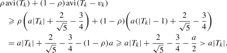
We plug these bounds into (8) and also use the identity (7) again. Since the expression (8) is linear in \(\rho \), its minimum is either attained for the largest or smallest possible value of \(\rho \). This gives us a lower bound for  in each of the aforementioned 105 cases, which can all be checked easily with a computer. As an example, let us consider the case that gives us the worst bound: it is obtained for \(x_1=x_3=x_4=0\), \(x_2=1\) and \(x_5=2\) (i.e., one branch with two vertices, two branches with four or more vertices). Let \(T_1\) and \(T_2\) both have four or more vertices, so that the third branch \(T_3\) consists of only two vertices. We have

and

as well as

by Lemma 4.3. Thus

and likewise

Plugging all these inequalities into (8), we obtain

The other cases are treated in the same fashion and give lower bounds with larger constant terms. To complete the proof of the theorem, it only remains to prove an upper bound on  . However, we already know from Lemma 4.2 that

for \(n > 3\), and \(\frac{\sqrt{5}}{2} - \frac{25}{26} \approx 0.15649553 < b\). Therefore,  for every tree T with n vertices other than \(P_n\).\(\square \)
5 A more general setting
It is common in statistical physics to consider the hard-core distribution on the independent sets I of a graph G. That is, the study of a random independent set I with probability proportional to \(\alpha ^{|I|}\). In [2, 3], the authors consider this model and prove bounds on the expected size of an independent set drawn from the hard-core model on G at fugacity \(\alpha \). When \(\alpha = 1\), this expected size is precisely the invariant  that we investigated in this paper. Recall that
  is the number of independent vertex subsets of size k in G. Now, choose a random independent set with probability proportional to \(\alpha ^k\), where k is the size of the set and \(\alpha \) is a positive number. We define the weighted total number of independent subsets of G, the weighted total size of independent subsets of G and the weighted average size of independent vertex subsets in G:

Example 5.1
For the n-vertex edgeless graph \(E_n\) and the star \(S_n\), we have

All the results presented in this paper, except for the extremality of the path, generalise to this weighted average.
Theorem 5.2
For any n-vertex graph G which is not the complete graph \(K_n\) and not the edgeless graph \(E_n\) we have  .
.
Theorem 5.3
For any n-vertex tree \(T\ne S_n\), we have  .
.
The proof that the path is extremal generalises to the case that \(\alpha \in (0,1]\), but not to all real values of \(\alpha \) (in fact, the path is not extremal for large values of \(\alpha \)).
Theorem 5.4
For every \(\alpha \in (0,1]\) and every tree T of order n, we have the inequality  .
.
To some extent, this also explains why proving extremality of the path is harder than proving extremality of the star. We refer to [11] for more details.
References
Brightwell, G.R., Winkler, P.: Hard constraints and the Bethe lattice: adventures at the interface of combinatorics and statistical physics. In: Tatsien, L.I. (ed.) Proceedings of the International Congress of Mathematicians, Vol. III (Beijing, 2002), pp. 605–624. Higher Education Press, Beijing (2002)
Davies, E., Jenssen, M., Perkins, W., Roberts, B.: Independent sets, matchings, and occupancy fractions. J. London Math. Soc. 96(1), 47–66 (2017)
Davies, E., Jenssen, M., Perkins, W., Roberts, B.: On the average size of independent sets in triangle-free graphs. Proc. Amer. Math. Soc. 146(1), 111–124 (2018)
Haslegrave, J.: Extremal results on average subtree density of series-reduced trees. J. Combin. Theory Ser. B 107, 26–41 (2014)
Jamison, R.E.: On the average number of nodes in a subtree of a tree. J. Combin. Theory Ser. B 35(3), 207–223 (1983)
Jamison, R.E.: Monotonicity of the mean order of subtrees. J. Combin. Theory Ser. B 37(1), 70–78 (1984)
Levit, V.E., Mandrescu, E.: The independence polynomial of a graph—a survey. In: Bozapalidis, S., Kalampakas, A., Rahonis, G. (eds.) Proceedings of the 1st International Conference on Algebraic Informatics, pp. 233–254. Aristotle University of Thessaloniki, Thessaloniki (2005)
Merrifield, R.E., Simmons, H.E.: Topological Methods in Chemistry. Wiley, New York (1989)
Mol, L., Oellermann, O.: Maximizing the mean subtree order. J. Graph Theory. https://doi.org/10.1002/jgt.22434
Prodinger, H., Tichy, R.F.: Fibonacci numbers of graphs. Fibonacci Quart. 20(1), 16–21 (1982)
Razanajatovo Misanantenaina, V.: Properties of Graph Polynomials and Related Parameters. PhD thesis, Stellenbosch University (2017)
Stephens, A.M., Oellermann, O.R.: The mean order of sub-\(k\)-trees of \(k\)-trees. J. Graph Theory 88(1), 61–79 (2018)
Vince, A., Wang, H.: The average order of a subtree of a tree. J. Combin. Theory Ser. B 100(2), 161–170 (2010)
Wagner, S.: Upper and lower bounds for Merrifield-Simmons index and Hosoya index. In: Gutman, I., Furtula, B., Das, K.C., Milovanović, E., Milovanović, I. (eds.) Bounds in Chemical Graph Theory—Basics. Mathematical Chemistry Monographs, vol. 19, pp. 155–187. University of Kragujevac, Kragujevac (2017)
Wagner, S., Wang, H.: On the local and global means of subtree orders. J. Graph Theory 81(2), 154–166 (2016)
Author information
Authors and Affiliations
Corresponding author
Additional information
Publisher's Note
Springer Nature remains neutral with regard to jurisdictional claims in published maps and institutional affiliations.
This work was supported by the National Research Foundation of South Africa (Grants 96236 and 96310).
Rights and permissions
About this article

Cite this article
Andriantiana, E.O.D., Razanajatovo Misanantenaina, V. & Wagner, S. The average size of independent sets of graphs. European Journal of Mathematics 6, 561–576 (2020). https://doi.org/10.1007/s40879-019-00333-8
Received:
Revised:
Accepted:
Published:
Issue Date:
DOI: https://doi.org/10.1007/s40879-019-00333-8