Multi-parameter Portfolio Selection Model with Some Novel Score-Deviation Under Dual Hesitant Fuzzy Environment

Abstract

In risk investment, investors have to rely on uncertain information when it is difficult to obtain enough precise data. Dual hesitant fuzzy set (DHFS) is more applicable to deal with uncertain information because it involves membership degrees and non-membership degrees, which can validly describe positive and negative information, respectively. Although there has been research on decision-making based on the DHFS, the focus still remains on ranking the alternatives and choosing the best one, which cannot help investors to find the optimal portfolios. Therefore, to solve this problem, we mainly propose two novel portfolio selection models based on the DHFS in this paper. Firstly, we propose a Max-score dual hesitant fuzzy portfolio selection model with information preference (Model 3) for investors focusing on returns regardless of risks. Secondly, to consider the risks of portfolios, we improve Model 3 and develop a score-deviation dual hesitant fuzzy portfolio selection model with information preference and risk appetite (Model 5). Finally, a case study is conducted to highlight the effectiveness of the proposed models. A detailed sensitivity analysis and an efficient frontier analysis show that Model 5 can validly capture investors’ information preferences and risk appetites. Furthermore, compared with the hesitant fuzzy portfolio model, Model 5 can offer more options to the investors with different information preferences.

1 Introduction

Markowitz’s mean–variance model [1] forms the foundation of the modern portfolio theory, which focuses on the relationship between returns and risks. Based on Markowitz’s theory, a lot of research has been carried out. Sharpe [2] simplified the mean–variance model by using stock market index. Mao [3] developed a mean-semi-variance model. Best and Hlouskova [4] took research on portfolio selection model with uncorrelated and bounded assets. Basak and Shapiro [5] explored the portfolio models with Value-at-Risk-Based risk management. However, most of these models above are based on precise data, which are sometimes difficult to obtain. Therefore, investors have to rely on qualitative data in real decision-making process.

To deal with uncertain information, fuzzy theories have been developed, such as the fuzzy set [6], the type-2 fuzzy set [7], the intuitionistic fuzzy set (IFS) [8], and the hesitant fuzzy set (HFS) [9]. Based on these fuzzy theories, some portfolio selection models have been proposed. Watada [10] studied the fuzzy portfolio selection and its application in decision-making. Tanaka and Guo [11] proposed a portfolio selection model based on upper and lower exponential possibility distributions. Deng and Pan [12] compared the multi-objective portfolio selection models based on intuitionistic fuzzy optimization. Zhou and Xu [13] proposed portfolio selection models for general investors and risk investors under hesitant fuzzy environment. Zhou et al. [14] developed a hesitant fuzzy portfolio selection model based on prospect theory to consider the psychological behaviors of experts.

Among fuzzy theories, the dual hesitant fuzzy set (DHFS) [15] is more applicable to describe uncertain information because it not only overcomes the IFS’s limitation that only one membership degree and one non-membership degree cannot comprehensively describe information, but also solves the HFS’s problem that membership degree is powerless to express both positive and negative information. Recently, the research on the DHFS has achieved great progress in three aspects. (1) Some basic concepts and operators are developed, including aggregation operators [16], distance and similarity measures [17], correlation coefficient measures [18] and entropy measures [19]. (2) Some extended theories based on the DHFS have been proposed, such as the probabilistic dual hesitant fuzzy set (PDHFS) [20], the dual hesitant fuzzy rough set (DHFRS) [21], and the dual hesitant bipolar fuzzy set (DHBFS) [22]. (3) Practical decision-making models have been developed, such as project assignment [23], teacher evaluation [24], and town selection for land policy [25].

The DHFS has also been applied in the investment area [26,27,28] to describe the information of stocks and help investors make investment decisions. However, it is worth noting that: (1) the models mentioned above mainly focus on selecting one stock or company to invest, but not on the portfolio selection under dual hesitant fuzzy environment. (2) Portfolio selection models based on the HFS [13] and IFS [29] have been properly proposed, but the similar model based on the DHFS cannot be found. It is well known that the DHFS is more valid in dealing with uncertain information. If the investment information is described by DHFSs and an investor wants to find an optimal portfolio, no applicable model can be used to satisfy the investor’s requirement. Therefore, to solve this problem, it is necessary to develop some new portfolio selection models based on the DHFS.

To build portfolio selection models based on the DHFS, investors have to evaluate stocks according to some criteria. Different criteria usually have different importance degrees, so determining criteria weights is necessary. Generally, criteria weights can be divided into two categories: subjective weights and objective weights. Subjective weights are derived from subjective preference information on criteria provided by decision-makers [30, 31]. In contrast, objective weights are obtained from the original evaluation information. One representative method of objective weights is the entropy method [32, 33], in which the criteria with bigger entropy values will be assigned smaller weights. Under dual hesitant fuzzy environment, there has also been some research on criteria weights [34,35,36]. In financial environment, it is difficult for investors to provide valid preference information on criteria because of the lack of precise data. Therefore, to better make use of the original information of DHFSs, the entropy method [32] is extended to dual hesitant fuzzy environment and used to calculate the objective weights of criteria in this paper.

When the information of stocks has been well processed, portfolio selection models can be built based on the DHFS. In this paper, we mainly propose two novel models under the dual hesitant fuzzy environment. Firstly, we propose a Max-score portfolio selection model (Model 3) for investors focusing on returns regardless of risks. In Model 3, a parameter $\alpha$ is defined to describe investors’ information preferences in terms of returns. Secondly, to consider the risks of portfolios, we improve Model 3 and develop a score-deviation portfolio selection model (Model 5) for investors with different information preferences and risk appetites. In Model 5, another two parameters $\zeta$ and $\beta$ are defined to describe investors’ risk appetites and information preferences in terms of risks, respectively. Finally, we conduct a case study to illustrate the effectiveness of the proposed models. A detailed sensitivity analysis and an efficient frontier analysis are conducted to show that Model 5 can validly capture investors’ information preferences and risk appetites. Moreover, Model 5 is compared with the hesitant fuzzy portfolio selection model to highlight its wider application.

This paper is organized as follows. In Sect. 2, the basic definitions and operations of the DHFS are reviewed. In Sect. 3, the calculation method of criteria weights based on the DHFS is illustrated. In Sect. 4, we propose a Max-score dual hesitant fuzzy portfolio selection model with information preference. In Sect. 5, we develop a score-deviation dual hesitant fuzzy portfolio selection model with information preference and risk appetite. In Sect. 6, two construction processes of the proposed portfolio selection models are summarized. In Sect. 7, a case study is conducted to show the availability of the proposed models. Conclusions are obtained in Sect. 8.

2 Preliminaries

In this section, we briefly introduce some important concepts about the DHFS and the basic operations of DHFSs. Then, we explain the definitions of returns and risks under dual hesitant fuzzy environment.

2.1 Dual Hesitant Fuzzy Set

Definition 1 [15]

Let $X$ be a fixed set, a DHFS $D$ on $X$ is described as:

$$ D = \left\{ {\left\langle {\left. {x,h(x),g(x)} \right\rangle |x \in X} \right.} \right\}, $$

(1)

where $h(x)$ and $g(x)$ are two sets of values in $[0,1]$, denoting the possible membership degrees and non-membership degrees of $x \in X$ to the set $D$, respectively, such that $\gamma \in h(x)$, $\eta \in g(x)$, $0\le \gamma , \, \eta \le 1$, $\gamma^{ + } = \text{max} \{ \gamma |\gamma \in h(x)\}$, $\eta^{ + } = \text{max} \{ \eta |\eta \in g(x)\}$ and $0 \le \gamma^{ + } + \eta^{ + } \le 1$. For convenience, the pair $d = \left\langle {\left. {h(x),g(x)} \right\rangle } \right.$ is called a dual hesitant fuzzy element (DHFE) and is denoted by $d = \left\langle {\left. {h,g} \right\rangle } \right.$.

Definition 2 [15]

Let $d = \left\langle {\left. {h,g} \right\rangle } \right.$ be a DHFE, the score function of $d$ is

$$ S = \frac{1}{\# h}\sum\limits_{\gamma \in h} \gamma - \frac{1}{\# g}\sum\limits_{\eta \in g} \eta , $$

(2)

where $\# h$ and $\# g$ are the numbers of elements in $h$ and $g$, respectively. Let $S_{h} = \frac{1}{\# h}\sum\nolimits_{\gamma \in h} \gamma$ and $S_{g} = \frac{1}{\# g}\sum\nolimits_{\eta \in g} \eta$, where $S_{h}$ is the mean of membership degrees and $S_{g}$ is the mean of non-membership degrees, then

$$ S = S_{h} - S_{g} . $$

(3)

Definition 3 [37]

Let $d = \left\langle {\left. {h,g} \right\rangle } \right.$ be a DHFE. Denote

$$ {\text{Std}}_{m} = \sqrt {\frac{1}{\# h}\sum\limits_{\gamma \in h} {(\gamma - S_{h} } )^{2} } $$

(4)

and

$$ {\text{Std}}_{n} = \sqrt {\frac{1}{\# g}\sum\limits_{\eta \in g} {(\eta - S_{g} } )^{2} } , $$

(5)

where ${\text{Std}}_{m}$ is the standard deviation of membership degrees of $d$ and ${\text{Std}}_{n}$ is the standard deviation of non-membership degrees of $d$. ${\text{Std}}_{m}$ and ${\text{Std}}_{n}$ reflect the degree of volatility when a decision-maker determines the values of elements in the DHFE. The larger the values of ${\text{Std}}_{m}$ and ${\text{Std}}_{n}$, the more volatile the data determined by the decision-maker.

According to Definition 3, we define the deviation of the DHFE as follows.

Definition 4

Let $d = \left\langle {\left. {h,g} \right\rangle } \right.$ be a DHFE, the deviation function of $d$ is

$$ V = \frac{1}{\# h}\sum\limits_{\gamma \in h} {(\gamma - S_{h} } )^{2} + \frac{1}{\# g}\sum\limits_{\eta \in g} {(\eta - S_{g} } )^{2} , $$

(6)

where $S_{h} = \frac{1}{\# h}\sum\nolimits_{\gamma \in h} \gamma$ and $S_{g} = \frac{1}{\# g}\sum\nolimits_{\eta \in g} \eta$. Let $V_{h} = \frac{1}{\# h}\sum\nolimits_{\gamma \in h} {(\gamma - S_{h} } )^{2}$ and $V_{g} = \frac{1}{\# g}\sum\nolimits_{\eta \in g} {(\eta - S_{g} } )^{2}$, where $V_{h}$ is the deviation of membership degrees and $V_{g}$ is the deviation of non-membership degrees, then

$$ V = V_{h} + V_{g} . $$

(7)

Let $d_{1}$ and $d_{2}$ be two DHFEs, the comparison laws between them are defined as follows:

• (1) If $S_{{d_{1} }} > S_{{d_{2} }}$, then $d_{1}$ is superior to $d_{2}$, denoted by $d_{1} \succ d_{2}$.

• (2) If $S_{{d_{1} }} < S_{{d_{2} }}$, then $d_{1}$ is inferior to $d_{2}$, denoted by $d_{1} \prec d_{2}$.

• (3) If $S_{{d_{1} }} = S_{{d_{2} }}$, then

  • (I) if $V_{{d_{1} }} < V_{{d_{2} }}$, then $d_{1} \succ d_{2}$;

  • (II) if $V_{{d_{1} }} > V_{{d_{2} }}$, then $d_{1} \prec d_{2}$;

  • (III) if $V_{{d_{1} }} = V_{{d_{2} }}$, then $d_{1}$ is equivalent to $d_{2}$, denoted by $d_{1} \sim d_{2}$.

2.2 Operations of DHFSs

Let $d_{1} = \left\langle {\left. {h_{1} ,g_{1} } \right\rangle } \right.$ and $d_{2} = \left\langle {\left. {h_{2} ,g_{2} } \right\rangle } \right.$ be two DHFEs, and $\lambda > 0$ be a parameter. The basic operations of them are defined as follows [15]:

• 1. $d_{1} \oplus d_{2} = \left\langle {\left. { \cup_{{\gamma_{1} \in h_{1} ,\gamma_{2} \in h_{2} }} \{ \gamma_{1} + \gamma_{2} - \gamma_{1} \gamma_{2} \} , \cup_{{\eta_{1} \in g_{1} ,\eta_{2} \in g_{2} }} \{ \eta_{1} \eta_{2} \} } \right \rangle } \right. ;$

• 2. $d_{1} \otimes d_{2} = \left\langle {\left. { \cup_{{\gamma_{1} \in h_{1} ,\gamma_{2} \in h_{2} }} \{ \gamma_{1} \gamma_{2} \} , \cup_{{\eta_{1} \in g_{1} ,\eta_{2} \in g_{2} }} \{ \eta_{1} + \eta_{2} - \eta_{1} \eta_{2} \} } \right\rangle } \right. ;$

• 3. $\lambda d_{1} = \left\langle {\left. { \cup_{{\gamma_{1} \in h_{1} }} \{ 1 - (1 - \gamma_{1} )^{\lambda } \} , \cup_{{\eta_{1} \in g_{1} }} \{ \eta_{1}^{\lambda } \} } \right\rangle } \right. ;$

• 4. $d_{1}^{\lambda } = \left\langle {\left. { \cup_{{\gamma_{1} \in h_{1} }} \{ \gamma_{1}^{\lambda } \} , \cup_{{\eta_{1} \in g_{1} }} \{ 1 - (1 - \eta_{1} )^{\lambda } \} } \right\rangle } \right..$

So far, the score function, deviation function, comparison laws and operations of DHFEs have been well defined. In the next section, the definitions of returns and risks in dual hesitant fuzzy portfolios are explained.

2.3 Returns and Risks Under Dual Hesitant Fuzzy Environment

According to Markowitz’s mean–variance model [1], the mean and variance of stock data represent the return and risk, respectively. However, statistics data are sometimes difficult to obtain and process in practical investment. For some new companies, there are even no useful data in the stock market, which makes it difficult to find the optimal investment proportions of new stocks. Therefore, proper definitions are needed to describe returns and risks under dual hesitant fuzzy environment.

Based on the model proposed by Zhou and Xu [13] and the definitions above, it can be found that Definition 2 is consistent with the definition of the mean. Meanwhile, Definition 4 describes the deviation degree from score value in a DHFE, which reflects the volatility degree of a decision-maker when he evaluates the stocks. The larger the value of deviation, the more volatile the data. Therefore, the score function of Eq. (3) and the deviation function of Eq. (7) are used to measure returns and risks, respectively, under dual hesitant fuzzy environment.

3 Calculation Method of Criteria Weights Based on Dual Hesitant Fuzzy Entropy

To better make use of the original information in DHFSs, we apply an entropy method to calculate the objective criteria weights in this paper. This method is similar to that proposed by Chen and Li [32]. The difference is that our method adopts dual hesitant fuzzy entropy, whereas the method of Chen and Li [32] adopts intuitionistic fuzzy entropy.

3.1 Entropy Measure of the DHFS

To determine the stability of the DHFS, Zhao and Xu [19] proposed an entropy measure. However, Ren et al. [25] pointed out that this entropy measure is not applicable when the numbers of elements in membership degree and non-membership degree are not equal, so they proposed a new entropy measure. In portfolio selection, the numbers of elements in membership degree and non-membership degree are generally different because of uncertainty. Therefore, the entropy [25] is used to calculate criteria weights in this paper.

Definition 5 [25]

Let $D$ be a DHFS, the entropy measure of $D$ can be defined as:

$$ E(D) = \frac{1}{m}\sum\limits_{i = 1}^{m} {\left( {\frac{1}{{(\# h_{{d_{i} }} ) \cdot (\# g_{{d_{i} }} )}}\sum\limits_{{\gamma \in h_{{d_{i} }} ,\eta \in g_{{d_{i} }} }} {\frac{{1 - |\gamma - \eta |^{\lambda } + (1 - \gamma - \eta )^{\lambda } }}{2}} } \right)} , $$

(8)

where $m$ is the number of DHFEs in $D$, $d_{i} = \left\langle {h_{{d_{i} }} ,g_{{d_{i} }} } \right\rangle$ is a DHFE in $D$. In this paper, let $\lambda = 1$, then the entropy measure of the DHFE $d_{i}$ can be denoted as:

$$ E(d_{i} ) = \frac{1}{{(\# h_{{d_{i} }} ) \cdot (\# g_{{d_{i} }} )}}\sum\limits_{{\gamma \in h_{{d_{i} }} ,\eta \in g_{{d_{i} }} }} {\frac{1 - |\gamma - \eta | + (1 - \gamma - \eta )}{2}} . $$

(9)

3.2 Calculation Process of Criteria Weights Based on Dual Hesitant Fuzzy Entropy

Assume that there are $m$ alternatives $A_{i} (i = 1,2, \ldots ,m)$ and $n$ criteria $C_{j} (i = 1,2, \ldots ,n)$. The dual hesitant fuzzy decision matrix $M$ is

(10)

where $d_{ij} = \left\langle {\left. {h_{ij} ,g_{ij} } \right\rangle } \right.$ is the performance value of $A_{i}$ under $C_{j}$.

• Step 1. Calculate the entropy value of each DHFE $d_{ij}$. Each performance value $d_{ij}$ in the decision matrix $M$ is then turned into an entropy value $E_{ij}$ based on Eq. (9). The entropy matrix $M_{0}$ is

  

  (11)

• Step 2. Calculate the criteria weights by applying the following transformation:

  $$ k_{j} = \frac{{1 - \sum\nolimits_{i = 1}^{m} {K_{ij} } }}{{n - \sum\nolimits_{j = 1}^{n} {\sum\nolimits_{i = 1}^{m} {K_{ij} } } }}, $$

  (12)

  where $k_{j}$ is the weight value of the criterion $C_{j}$·$K_{ij}$ is the normalized value of $E_{ij}$ based on Eq. (13):

  $$ K_{ij} = \frac{{E_{ij} }}{{\mathop {\text{max} }\limits_{i} (E_{ij} )}}. $$

  (13)

There is another dual hesitant fuzzy entropy method proposed by Chen et al. [36], which normalizes $E_{ij}$ based on $K_{ij} = \frac{{E_{ij} }}{m}$. It is obvious that $\sum\nolimits_{i = 1}^{m} {K_{ij} } = \frac{1}{m}\sum\nolimits_{i = 1}^{m} {E_{ij} }$ focuses on averaging the entropy values under each criterion. However, our method normalizes $E_{ij}$ by using Eq. (13), which measures the closeness of $E_{ij}$ to the maximum entropy value under the criterion $C_{j}$. In risk investment, the stock with the highest entropy value is the most unstable and can be an important reference point for decision-makers. Therefore, Eq. (13) is more suitable and adopted in this paper. Next, an example is given to illustrate the calculation process of our entropy method.

Example 1

Assume that there are two alternatives $A_{i} (i = 1,2)$ and two criteria $C_{j} (i = 1,2)$. The dual hesitant fuzzy decision matrix $M$ is

• Step 1. The entropy matrix $M_{0}$ is

  

  where $E_{11} = \frac{1}{2} \cdot \frac{1 - |0.3 - 0.5| + (1 - 0.3 - 0.5) + 1 - |0.4 - 0.5| + (1 - 0.4 - 0.5)}{2} = 0.5$ and other entropy values can be obtained similarly based on Eq. (9).

• Step 2. The weight values of $C_{ 1}$ and $C_{2}$ are 0.5455 and 0.4545, respectively, where $k_{1} = \frac{1}{2 - 3.65} \cdot \left[ {1 - \left( {\frac{0.5}{0.5} + \frac{0.45}{0.5}} \right)} \right] = 0.5455$ and $k_{2} = \frac{1}{2 - 3.65} \cdot \left[ {1 - \left( {\frac{0.6}{0.6} + \frac{0.45}{0.6}} \right)} \right] = 0.4545.$

4 Max-Score Dual Hesitant Fuzzy Portfolio Selection Model with Information Preference

In Sect. 2, returns and risks under dual hesitant fuzzy environment have been well defined. In this section, we suppose that investors only want to obtain the maximum returns without taking into account the risks, so we propose a Max-score portfolio selection model with information preference under dual hesitant fuzzy environment.

4.1 Max-Score Dual Hesitant Fuzzy Portfolio Selection Model

In this section, we propose a Max-score dual hesitant fuzzy portfolio selection model. Assume that there are $m$ new stocks $\{ a_{1} ,a_{2} , \ldots ,a_{i} , \ldots ,a_{m} \}$ and $n$ criteria $\{ C_{1} ,C_{2} , \ldots ,C_{j} , \ldots ,C_{n} \}$. An investor wants to put a fund on these stocks, but cannot get enough quantitative data. Therefore, the investor collects qualitative data represented by a dual hesitant fuzzy matrix $M = [d_{ij} ]_{m \times n}$, where $d_{ij} = \left\langle {\left. {h_{ij} ,g_{ij} } \right\rangle } \right.(i = 1,2, \ldots ,m;j = 1,2, \ldots ,n)$ refers to the dual hesitant fuzzy information of the stock $a_{i}$ with respect to the criterion $C_{j}$. Firstly, the criteria weights $k_{j} (j = 1,2, \ldots ,n)$ can be obtained based on the entropy method in Sect. 3. Then, the DHFEs of each stock are aggregated and the dual hesitant fuzzy matrix $M = [d_{ij} ]_{m \times n}$ is transformed into an aggregated decision matrix $\overline{M} = [\overline{{d_{i} }} ]_{m \times 1}$ based on Eq. (14), where $\overline{{d_{i} }} (i = 1,2, \ldots ,m)$ is the aggregated DHFE of the stock $a_{i}$.

$$ \overline{{d_{i} }} = \left\langle {\overline{{h_{i} }} ,\overline{{g_{i} }} } \right\rangle = \oplus_{{{\text{j}} = 1}}^{n} k_{j} d_{ij} = \left\langle { \cup_{{\gamma_{ij} \in h_{ij} }} \{ 1 - \prod\limits_{j = 1}^{n} {(1 - \gamma_{ij} )^{{k_{j} }} } \} , \cup_{{\eta_{ij} \in g_{ij} }} \left \{ \prod\limits_{j = 1}^{n} {\eta_{ij}^{{k_{j} }} } \right \} } \right\rangle . $$

(14)

Finally, the optimal investment proportions can be obtained by using Model 1.

Model 1

$$ \begin{aligned} & \text{max} \, R(W) = S( \oplus_{i = 1}^{m} w_{i} \overline{{d_{i} }} ) \hfill \\ & {\text{s}} . {\text{t}} .\left\{ \begin{aligned} & \sum\limits_{i = 1}^{m} {w_{i} } \le 1 \hfill \\ & w_{i} \ge 0,i = 1,2, \ldots ,m \hfill \\ \end{aligned} \right., \hfill \\ \end{aligned} $$

(15)

where $\oplus_{i = 1}^{m} w_{i} \overline{{d_{i} }} = \left\langle { \cup_{{\overline{{\gamma_{i} }} \in \overline{{h_{i} }} }} \{ 1 - \prod\nolimits_{i = 1}^{m} {(1 - \overline{{\gamma_{i} }} )^{{w_{i} }} } \} , \cup_{{\overline{{\eta_{i} }} \in \overline{{g_{i} }} }} \{ \prod\nolimits_{i = 1}^{m} {\overline{\eta }_{i}^{{w_{i} }} } \} } \right\rangle$ is the aggregated DHFE of a portfolio, $R(W)$ describes the portfolio return, $S( \oplus_{i = 1}^{m} w_{i} \overline{{d_{i} }} )$ is the score function of $\oplus_{i = 1}^{m} w_{i} \overline{{d_{i} }}$ based on Eq. (3), $k_{\text{j}}$ is the weight value of the criterion $C_{j}$, and $w_{i}$ is the optimal investment proportion of the stock $a_{i}$.

Theorem 1

The constraint condition $\sum\nolimits_{i = 1}^{m} {w_{i} = 1}$ is equivalent to $\sum\nolimits_{i = 1}^{m} {w_{i} \le 1}$ in Model 1.

Proof

Let $W_{ 0} = \{ w_{i}^{*} \} ,i = 1,2, \ldots ,m$ be a feasible solution to Model 1 and $\sum\nolimits_{i = 1}^{m} {w_{i}^{*} } < 1$. Then, the return of Model 1 at $W_{ 0}$ is

$$ R(W_{0} ) = S \left(\left\langle { \cup_{{\overline{{\gamma_{i} }} \in \overline{{h_{i} }} }} \left \{ 1 - \prod\limits_{i = 1}^{m} {(1 - \overline{{\gamma_{i} }} )^{{w_{i}^{*} }} } \right \} , \cup_{{\overline{{\eta_{i} }} \in \overline{{g_{i} }} }} \left \{ \prod\limits_{i = 1}^{m} {\overline{\eta }_{i}^{{w_{i}^{*} }} } \right \} } \right\rangle \right) . $$

(16)

Next, we will show $W^{ *} = (w_{1}^{*} , \ldots ,w_{i - 1}^{*} ,1 - \sum\nolimits_{j \ne i} {w_{j}^{*} } ,w_{i + 1}^{*} , \ldots ,w_{m} )$ is a better solution than $W_{ 0}$. Based on Eq. (3), we have

$$ R(W^{*} ) = S\left( {\left\langle { \cup_{{\overline{{\gamma_{i} }} \in \overline{{h_{i} }} }} \left \{ 1 - (1 - \overline{{\gamma_{i} }} )^{{1 - \sum\limits_{j \ne i}^{m} {w_{j}^{*} } }} \prod\limits_{j \ne i}^{m} {(1 - \overline{{\gamma_{j} }} )^{{w_{j}^{*} }} } \right \} , \cup_{{\overline{{\eta_{i} }} \in \overline{{g_{i} }} }} \left \{ \overline{\eta }_{i}^{{1 - \sum\limits_{j \ne i}^{m} {w_{j}^{*} } }} \prod\limits_{j \ne i}^{m} {\overline{\eta }_{j}^{{w_{j}^{*} }} }\right \} } \right\rangle } \right) . $$

(17)

Since $\sum\nolimits_{i = 1}^{m} {w_{i}^{*} } < 1$ and $0\le \overline{{\gamma_{i} }} , \, \overline{{\eta_{i} }} \le 1$, we have $1 - \sum\nolimits_{j \ne i}^{m} {w_{j}^{*} } > w_{i}^{*}$,

$$ 1 - (1 - \overline{{\gamma_{i} }} )^{{1 - \sum\limits_{j \ne i}^{m} {w_{j}^{*} } }} \prod\limits_{j \ne i}^{m} {(1 - \overline{{\gamma_{j} }} )^{{w_{j}^{*} }} } \ge 1 - (1 - \overline{{\gamma_{i} }} )^{{w_{i}^{*} }} \prod\limits_{j \ne i}^{m} {(1 - \overline{{\gamma_{j} }} )^{{w_{j}^{*} }} } $$

(18)

and

$$ \overline{\eta }_{i}^{{1 - \sum\limits_{j \ne i}^{m} {w_{j}^{*} } }} \prod\limits_{j \ne i}^{m} {\overline{\eta }_{j}^{{w_{j}^{*} }} } \le \overline{\eta }_{i}^{{w_{i}^{*} }} \prod\limits_{j \ne i}^{m} {\overline{\eta }_{j}^{{w_{j}^{*} }} } . $$

(19)

Therefore, $R(W^{ *} ) \ge R(W_{0} )$. Then, the constraint condition $\sum\nolimits_{i = 1}^{m} {w_{i} \le 1}$ is equivalent to $\sum\nolimits_{i = 1}^{m} {w_{i} = 1}$.

According to Theorem 1, Model 1 can be transformed into Model 2:

Model 2

$$ \begin{aligned} & \text{max} \, R(W) = S( \oplus_{i = 1}^{m} w_{i} \overline{{d_{i} }} ) \hfill \\ & {\text{s}} . {\text{t}} .\left\{ \begin{aligned} & \sum\limits_{i = 1}^{m} {w_{i} } = 1 \hfill \\ & w_{i} \ge 0,i = 1,2, \ldots ,m \hfill \\ \end{aligned} \right.. \hfill \\ \end{aligned} $$

(20)

For convenience, we denote $\oplus_{i = 1}^{m} w_{i} \overline{{d_{i} }}$ as

$$ D_{R} = \left\langle {H,G} \right\rangle , $$

(21)

where $H = \cup_{{\overline{{\gamma_{i} }} \in \overline{{h_{i} }} }} \{ 1 - \prod\limits_{i = 1}^{m} {(1 - \overline{{\gamma_{i} }} )^{{w_{i} }} } \}$ and $G = \cup_{{\overline{{\eta_{i} }} \in \overline{{g_{i} }} }} \{ \prod\limits_{i = 1}^{m} {\overline{\eta }_{i}^{{w_{i} }} } \}$. Let

$$ R(W) = S\left( {\left\langle { \cup_{{\overline{{\gamma_{i} }} \in \overline{{h_{i} }} }} \{ 1 - \prod\limits_{i = 1}^{m} {(1 - \overline{{\gamma_{i} }} )^{{w_{i} }} } \} , \cup_{{\overline{{\eta_{i} }} \in \overline{{g_{i} }} }} \{ \prod\limits_{i = 1}^{m} {\overline{\eta }_{i}^{{w_{i} }} } \} } \right\rangle } \right) = S_{H} (W) - S_{G} (W) , $$

(22)

where

$$ S_{H} (W) = \frac{1}{{l_{H} }}\sum\limits_{u = 1}^{{l_{H} }} {s_{u} (W)} , $$

(23)

$$ S_{G} (W) = \frac{1}{{l_{G} }}\sum\limits_{e = 1}^{{l_{G} }} {s_{e} } (W) , $$

(24)

$s_{u} (W) = 1 - \prod\nolimits_{i = 1}^{m} {(1 - \overline{{\gamma_{i} }} )^{{w_{i} }} }$, $s_{\text{e}} (W) = \prod\nolimits_{i = 1}^{m} {\overline{\eta }_{i}^{{w_{i} }} }$, $l_{H}$ is the number of elements in $H$ and $l_{G}$ is the number of elements in $G$.

Lemma 1 (Weierstrass’ Theorem [38, Proposition A.8])

Let$T$be a nonempty subset of${\mathbb{R}}^{n}$, the n-dimensional Euclidean space, if$f:T \mapsto {\mathbb{R}}$is upper semi-continuous at all points of$T$and$T$is closed and bounded, then there exists a vector$x \in T$such that$f(x) = \sup_{z \in T} f(z)$.

Remark 1

If $f:T \mapsto {\mathbb{R}}$ is a continuous function, then $f$ is upper semi-continuous.

Theorem 2

Model 2 has a globally optimal solution.

Proof

In Model 2, let $D_{w} = \left\{ {W = (w_{1} , \ldots ,w_{2} , \ldots w_{m} )^{T} |\sum\nolimits_{i = 1}^{m} {w_{i} = 1} \, , \, w_{i} \ge 0} \right\}$. It is obvious that $D_{w}$ is closed and bounded. In addition, since a function composed of a finite number of exponential functions and constants is continuous, $s_{u} (W) = 1 - \prod\nolimits_{i = 1}^{m} {(1 - \overline{{\gamma_{i} }} )^{{w_{i} }} }$ and $s_{\text{e}} (W) = \prod\nolimits_{i = 1}^{m} {\overline{\eta }_{i}^{{w_{i} }} }$ are continuous when $0\le \overline{{\gamma_{i} }} , \, \overline{{\eta_{i} }} \le 1$. Then, we can derive from Eqs. (22)–(24) that $R(W)$ is continuous on $D_{w}$. Therefore, Model 2 is well defined and has a globally optimal solution according to Lemma 1.

Theorem 3

The objective function of Model 2 is a concave function.

Proof

To prove the theorem, we need to prove that the Hessian matrix of $R(W)$ is a negative semi-definite matrix. According to Eq. (22), if we can prove that the Hessian matrix of $S_{H} (W)$ is a negative semi-definite matrix and the Hessian matrix of $S_{G} (W)$ is a positive semi-definite matrix, we will prove the theorem. Consider the second-order mixed partial derivative of $R(W)$:

$$ \frac{{\partial^{ 2} R(W)}}{{\partial w_{i} \partial w_{j} }} = \frac{{\partial^{ 2} S_{H} (W)}}{{\partial w_{i} \partial w_{j} }} - \frac{{\partial^{ 2} S_{G} (W)}}{{\partial w_{i} \partial w_{j} }} = \frac{1}{{l_{H} }}\sum\limits_{u = 1}^{{l_{H} }} {\frac{{\partial^{ 2} s_{u} (W)}}{{\partial w_{i} \partial w_{j} }} - } \frac{1}{{l_{G} }}\sum\limits_{e = 1}^{{l_{G} }} {\frac{{\partial^{ 2} s_{e} (W)}}{{\partial w_{i} \partial w_{j} }}} . $$

(25)

Since $s_{u} (W)$ and $s_{e} (W)$ are all positive, we can just consider $\frac{{\partial^{ 2} s_{u} (W)}}{{\partial w_{i} \partial w_{j} }}$ and $\frac{{\partial^{ 2} s_{e} (W)}}{{\partial w_{i} \partial w_{j} }}$.

Firstly, consider the Hessian matrix of $s_{u} (W)$. Since

$$ \frac{{\partial^{ 2} s_{u} (W)}}{{\partial w_{i}^{2} }} = - (\ln (1 - \overline{{\gamma_{i} }} ))^{2} \prod\limits_{i = 1}^{m} {(1 - \overline{{\gamma_{i} }} )^{{w_{i} }} } $$

(26)

and

$$ \frac{{\partial^{ 2} s_{u} (W)}}{{\partial w_{i} \partial w_{j} }} = - \ln (1 - \overline{{\gamma_{i} }} )\ln (1 - \overline{{\gamma_{j} }} )\prod\limits_{i = 1}^{m} {(1 - \overline{{\gamma_{i} }} )^{{w_{i} }} } , $$

(27)

the Hessian matrix of $s_{u} (W)$ is

$$ H_{u} = \left[ {\begin{array}{*{20}c} {\frac{{\partial^{2} s_{u} (W)}}{{\partial w_{1}^{2} }}} & \cdots & {\frac{{\partial^{2} s_{u} (W)}}{{\partial w_{1} \partial w_{i} }}} & \cdots & {\frac{{\partial^{2} s_{u} (W)}}{{\partial w_{1} \partial w_{m} }}} \\ \vdots & \cdots & \vdots & \cdots & \vdots \\ {\frac{{\partial^{2} s_{u} (W)}}{{\partial w_{i} \partial w_{1} }}} & \cdots & {\frac{{\partial^{2} s_{u} (W)}}{{\partial w_{i}^{2} }}} & \cdots & {\frac{{\partial^{2} s_{u} (W)}}{{\partial w_{i} \partial w_{m} }}} \\ \vdots & \cdots & \vdots & \cdots & \vdots \\ {\frac{{\partial^{2} s_{u} (W)}}{{\partial w_{m} \partial w_{1} }}} & \cdots & {\frac{{\partial^{2} s_{u} (W)}}{{\partial w_{m} \partial w_{i} }}} & \cdots & {\frac{{\partial^{2} s_{u} (W)}}{{\partial w_{m}^{2} }}} \\ \end{array} } \right] . $$

(28)

It is obvious that $H_{u}$ can be transformed into:

$$ H_{u} = AA^{T} \cdot ( - \prod\limits_{i = 1}^{m} {(1 - \overline{{\gamma_{i} }} )^{{w_{i} }} } ) , $$

(29)

where $A = (\ln (1 - \overline{{\gamma_{1} }} ), \ldots ,\ln (1 - \overline{{\gamma_{i} }} ), \ldots ,\ln (1 - \overline{{\gamma_{m} }} ))^{T}$ and $AA^{T}$ is a positive semi-definite matrix. Therefore, $H_{u}$ is a negative semi-definite matrix.

Secondly, consider the Hessian matrix of $s_{e} (W)$ similarly. Since

$$ \frac{{\partial^{ 2} s_{e} (W)}}{{\partial w_{i}^{2} }} = (\ln \overline{\eta }_{i} )^{2} \prod\limits_{i = 1}^{m} {\overline{\eta }_{i}^{{w_{i} }} } $$

(30)

and

$$ \frac{{\partial^{ 2} s_{e} (W)}}{{\partial w_{i} \partial w_{j} }} = \ln \overline{\eta }_{i} \ln \overline{\eta }_{j} \prod\limits_{i = 1}^{m} {\overline{\eta }_{i}^{{w_{i} }} } , $$

(31)

the Hessian matrix of $s_{e} (W)$ is

$$ H_{e} = BB^{T} \cdot \prod\limits_{i = 1}^{m} {\overline{\eta }_{i}^{{w_{i} }} } , $$

(32)

where $B = (\ln \overline{\eta }_{1} , \ldots ,\ln \overline{\eta }_{i} ,\; \ldots ,\ln \overline{\eta }_{m} )^{T}$ and $BB^{T}$ is a positive semi-definite matrix. Therefore, $H_{e}$ is a positive semi-definite matrix and $- H_{e}$ is a negative semi-definite matrix. Finally, we can derive from Eq. (25) that the Hessian matrix of $R(W)$ is a negative semi-definite matrix, so the objective function of Model 2 is a concave function.

4.2 Max-Score Dual Hesitant Fuzzy Portfolio Selection Model with Information Preference

As discussed above, the membership degrees and non-membership degrees in the DHFS can represent positive and negative information, respectively. In practical investment, investors usually hold different attitudes to positive and negative information. Therefore, Model 3 is constructed based on Model 2 to incorporate investors’ information preferences.

Model 3

$$ \begin{aligned} & \text{max} \, R(W) = \alpha S_{H} (W) - (1 - \alpha )S_{G} (W) \hfill \\ & {\text{s}} . {\text{t}} .\left\{ \begin{aligned} & \sum\limits_{i = 1}^{m} {w_{i} } = 1 \hfill \\ & w_{i} \ge 0,i = 1,2, \ldots ,m \hfill \\ \end{aligned} \right., \hfill \\ \end{aligned} $$

(33)

where $0 \le \alpha \le 1$. The parameter $\alpha$ describes the investor’s information preference and its value is determined by the investor. From the proof of Theorem 2, we can obtain that the function being maximized in Model 3 is continuous on $D_{w}$, so Model 3 has a globally optimal solution according to Lemma 1.

Corollary 1

The constraint condition $\sum\nolimits_{i = 1}^{m} {w_{i} \le 1}$ is equivalent to $\sum\nolimits_{i = 1}^{m} {w_{i} = 1}$ in Model 3.

Proof

Let $W_{ 0} = \{ w_{i}^{*} \} ,i = 1,2, \ldots ,m$ be a feasible solution to Model 3 such that $\sum\nolimits_{i = 1}^{m} {w_{i}^{*} } < 1$, and $W^{ *} = (w_{1}^{*} , \ldots ,w_{i - 1}^{*} ,1 - \sum\limits_{j \ne i} {w_{j}^{*} } ,w_{i + 1}^{*} , \ldots ,w_{m} )$. Since $0 \le \alpha \le 1$, we can derive from the proof of Theorem 1 that $\alpha S_{H} (W^{ *} ) \ge \alpha S_{H} (W_{0} )$, $(1 - \alpha )S_{G} (W^{ *} ) \le (1 - \alpha )S_{G} (W_{0} )$ and $R(W^{ *} ) \ge R(W_{0} )$. Therefore, the constraint conditions $\sum\nolimits_{i = 1}^{m} {w_{i} = 1}$ and $\sum\nolimits_{i = 1}^{m} {w_{i} \le 1}$ are equivalent.

Theorem 4

The objective function of Model 3 is a concave function. Moreover, Model 3 is equivalent to a convex programming.

Proof

According to Eq. (25), it is obvious that the second-order mixed partial derivative of $R(W)$ in Model 3 is $\frac{{\partial^{ 2} R(W)}}{{\partial w_{i} \partial w_{j} }} = \alpha \frac{{\partial^{ 2} S_{H} (W)}}{{\partial w_{i} \partial w_{j} }} - \left( {1 - \alpha } \right)\frac{{\partial^{ 2} S_{G} (W)}}{{\partial w_{i} \partial w_{j} }}$. Since $0 \le \alpha \le 1$, we can derive from the proof of Theorem 3 that the Hessian matrix of $\alpha S_{H} (W)$ is a negative semi-definite matrix and the Hessian matrix of $\left( {1 - \alpha } \right)S_{G} (W)$ is a positive semi-definite matrix. Then, the Hessian matrix of $R(W)$ in Model 3 is a negative semi-definite matrix. Therefore, the objective function of Model 3 is a concave function and $- R(W)$ is a convex function.

Note that Eq. (33) and Eq. (34) are equivalent.

$$ \begin{aligned} & \text{min} \, - R(W) = (1 - \alpha )S_{G} (W) - \alpha S_{H} (W) \hfill \\ & {\text{s}} . {\text{t}} .\left\{ \begin{aligned} & \sum\limits_{i = 1}^{m} {w_{i} } = 1 \hfill \\ & w_{i} \ge 0,i = 1,2, \ldots ,m \hfill \\ \end{aligned} \right. \hfill \\ \end{aligned} $$

(34)

Since the objective function is a convex function and the constraint conditions are linear functions, Eq. (34) is a convex programming. Therefore, Eq. (33) is equivalent to a convex programming and has some good properties similar to those of Eq. (34). For example, any local optimum is a global optimum according to optimization theory.

Property 1

Different values of $\alpha$ in Model 3 represent investors’ different information preferences in terms of returns.

• (1) If $0.5 < \alpha \le 1$, investors pay more attention to positive information;

• (2) If $0 \le \alpha < 0.5$, investors pay more attention to negative information;

• (3) If $\alpha = 0.5$, the importance degrees of positive and negative information are equal, and Model 3 is equivalent to Model 2;

• (4) If $\alpha = 1$, Model 3 will be similar to the hesitant fuzzy portfolio selection model for general investors proposed by Zhou and Xu [13].

5 Score-Deviation Dual Hesitant Fuzzy Portfolio Selection Model with Information Preference and Risk Appetite

In Sect. 4, we have proposed the Max-score portfolio selection model with information preference (Model 3). However, Model 1, Model 2 and Model 3 only focus on maximizing the return, but ignore the risk in portfolio selection. It is well known that investors also want to avoid risks as much as they can in their pursuit of the maximum returns. Therefore, we improve Model 3 by considering both returns and risks.

5.1 Score-Deviation Dual Hesitant Fuzzy Portfolio Selection Model with Information Preference

For convenience, we firstly develop a bi-objective portfolio selection model with information preference, which is described as Model 4.

Model 4

$$ \begin{aligned} & { \text{max} }R(W) = \alpha S_{H} (W) - (1 - \alpha )S_{G} (W) \hfill \\ & { \text{min} }V(W) = \beta V_{H} (W) + (1 - \beta )V_{G} (W) \hfill \\ & {\text{s}} . {\text{t}} .\left\{ \begin{aligned} & \sum\limits_{i = 1}^{m} {w_{i} } = 1 \hfill \\ & w_{i} \ge 0,i = 1,2, \ldots ,m \hfill \\ \end{aligned} \right., \hfill \\ \end{aligned} $$

(35)

where $0 \le \alpha \le 1$, $0 \le \beta \le 1$,

$$ V_{H} (W) = \frac{1}{{l_{H} }}\sum\limits_{u = 1}^{{l_{H} }} {(s_{u} (W) - S_{H} (W))^{2} } , $$

(36)

$$ V_{G} (W) = \frac{1}{{l_{G} }}\sum\limits_{e = 1}^{{l_{G} }} {(s_{e} (W) - S_{G} (W))^{2} } , $$

(37)

and $V(W)$ describes the portfolio risk. The parameter $\alpha$ is the same as that in Model 3. Since investors’ information preferences in terms of returns and risks may be different, the parameter $\beta$ is defined to describe the investor’s information preference in terms of risks. The value of $\beta$ is determined by the investor.

Property 2

Different values of $\beta$ in Model 4 represent investors’ different information preferences in terms of risks:

• (1) If $0.5 < \beta \le 1$, investors pay more attention to positive information;

• (2) If $0 \le \beta < 0.5$, investors pay more attention to negative information;

• (3) If $\beta = 0.5$, the importance degrees of positive and negative information are equal;

• (4) If $\beta = 1$ and $\alpha = 1$, Model 4 will be similar to the hesitant fuzzy portfolio selection model for risk investors proposed by Zhou and Xu [13].

5.2 Score-Deviation Dual Hesitant Fuzzy Portfolio Selection Model with Information Preference and Risk Appetite

It is obvious that returns and risks are of the same importance in Model 4, which is not consistent with the consensus that investors usually have different risk appetites. Therefore, Model 5 is constructed based on Model 4 to incorporate investors’ risk appetites.

Model 5

$$ \begin{aligned} & { \text{max} }R(W) = \alpha S_{H} (W) - (1 - \alpha )S_{G} (W) \hfill \\ & {\text{s}} . {\text{t}}\left\{ \begin{aligned} & V(W) \le \zeta \hfill \\ & \sum\limits_{i = 1}^{m} {w_{i} } = 1 \hfill \\ & w_{i} \ge 0,i = 1,2, \ldots ,m \hfill \\ \end{aligned} \right., \hfill \\ \end{aligned} $$

(38)

where $V(W) = \beta V_{H} (W) + (1 - \beta )V_{G} (W)$, $0 \le \alpha \le 1$, $0 \le \beta \le 1$, $\zeta$ describes the investor’s risk appetite, and $\zeta \in [V_{\text{min} } ,V_{\text{max} } ]$. When the value of $\beta$ is given according to the investor’s information preference, we have

$$ \begin{aligned} & V_{\text{max} } = \text{max} \, V(W) \hfill \\ & {\text{s}} . {\text{t}}\left\{ \begin{aligned} & \sum\limits_{i = 1}^{m} {w_{i} } = 1 \hfill \\ & w_{i} \ge 0,i = 1,2, \ldots ,m \hfill \\ \end{aligned} \right., \hfill \\ \end{aligned} $$

(39)

and

$$ \begin{aligned} & V_{\text{min} } = \text{min} \, V(W) \hfill \\ & {\text{s}} . {\text{t}} .\left\{ \begin{aligned} & \sum\limits_{i = 1}^{m} {w_{i} } = 1 \hfill \\ & w_{i} \ge 0,i = 1,2, \cdots ,m \hfill \\ \end{aligned} \right. \hfill \\ \end{aligned} , $$

(40)

where $V_{\text{max} }$ and $V_{\text{min} }$ are the maximum risk value and the minimum risk value of the portfolio, respectively.

Theorem 5

Model 5 has a globally optimal solution.

Proof

Let $T = \left\{ {W = (w_{1} , \ldots ,w_{2} , \ldots ,w_{m} )^{T} \left| {V(W) = \beta V_{H} + (1 - \beta )V_{G} \le \zeta } \right.} \right\}$, where the value of $\zeta$ is given by the investor, and $D_{w} = \left\{ {W = (w_{1} , \ldots ,w_{2} , \ldots ,w_{m} )^{T} |\sum\nolimits_{i = 1}^{m} {w_{i} = 1} \, , \, w_{i} \ge 0} \right\}$. It is obvious that $T \cap D_{w}$ is bounded. Next, we will prove that $T \cap D_{w}$ is closed.

Let $\left\{ {W^{k} = (w_{{_{1} }}^{k} , \ldots ,w_{{_{2} }}^{k} , \ldots ,w_{{_{m} }}^{k} )^{T} } \right\}$ be an arbitrarily convergent sequence of elements in $T$ such that $\mathop {\lim }\nolimits_{k \to \infty } W^{k} = \overline{W}$. Since $s_{u} (W) = 1 - \prod\nolimits_{i = 1}^{m} {(1 - \overline{{\gamma_{i} }} )^{{w_{i} }} }$ and $s_{\text{e}} (W) = \prod\nolimits_{i = 1}^{m} {\overline{\eta }_{i}^{{w_{i} }} }$ are continuous when $0\le \overline{{\gamma_{i} }} , \, \overline{{\eta_{i} }} \le 1$, we can derive from Eq. (36) and Eq. (37) that $V(W)$ is continuous. By mathematical analysis, it is easily verified that $V(\overline{W} ) = \mathop {\lim }\nolimits_{{W \to \overline{W} }} V(W) = \mathop {\lim }\nolimits_{k \to \infty } V(W^{k} ) \le \zeta$. That is to say, $\overline{W} \in T$ and $T$ is a closed set. Since $D_{w}$ is closed, $T \cap D_{w}$ is closed. In addition, we can derive from the proof of Theorem 2 that the function being maximized in Model 5 is continuous on $T \cap D_{w}$, so Model 5 is well defined and has a globally optimal solution according to Lemma 1.

Property 3

Different values of$\zeta$in Model 5 represent investors’ different risk appetites. By trisecting the range$[V_{\text{min} } ,V_{\text{max} } ]$, we can obtain that:

• (1) if $V_{\text{min} } \le \zeta \le V_{\text{min} } + \frac{1}{3}\left( {V_{\text{max} } - V_{\text{min} } } \right)$, investors are risk-averse;

• (2) if $V_{\text{min} } + \frac{1}{3}(V_{\text{max} } - V_{\text{min} } ) < \zeta \le V_{\text{min} } + \frac{2}{3}(V_{\text{max} } - V_{\text{min} } )$, investors are risk-neutral;

• (3) if $V_{\text{min} } + \frac{2}{3}(V_{\text{max} } - V_{\text{min} } ) < \zeta \le V_{\text{max} }$, investors are risk-seeking;

• (4) if $\zeta = V_{\text{max} }$, Model 5 will be the same as Model 3.

So far, we have proposed the Max-score dual hesitant fuzzy portfolio selection model with information preference and the score-deviation dual hesitant fuzzy portfolio selection model with information preference and risk appetite. In the next section, we summarize the portfolio selection process under dual hesitant fuzzy environment.

6 Portfolio Selection Process Under Dual Hesitant Fuzzy Environment

Assume that there are $m$ new stocks $\{ a_{1} ,a_{2} , \ldots a_{i} , \ldots ,a_{m} \}$ and $n$ criteria $\{ C_{1} ,C_{2} , \ldots C_{j} , \ldots ,C_{n} \}$. An investor wants to put a fund on these stocks, but cannot get enough quantitative data. Thus, the investor has to collect qualitative data from some experts, who evaluate the stocks based on the DHFS. The evaluation information of the stocks is represented by a dual hesitant fuzzy matrix $M = [d_{ij} ]_{m \times n}$, where $d_{ij} = \left\langle {\left. {h_{ij} ,g_{ij} } \right\rangle } \right.(i = 1,2, \ldots ,m;j = 1,2, \cdots ,n)$ is a DHFE describing the dual hesitant fuzzy information of the stock $a_{i}$ with respect to the criterion $C_{j}$. To help the investor find the optimal investment proportions, a suitable portfolio selection process based on the DHFS is needed. Generally, portfolio selection process can be divided into two categories: Process I for investors focusing on returns regardless of risks and Process II for investors considering both returns and risks. Next, the details of the two processes under dual hesitant fuzzy environment are explained.

Process I

According to the discussion above, it is obvious that Models 1-3 are suitable for Process I. However, it has been verified that (1) Model 1 is equivalent to Model 2 by Theorem 1. (2) Model 3 considers information preference, which is not considered in the other two models. (3) According to Property 1, Model 3 is equivalent to Model 2 when $\alpha = 0.5$. Therefore, Model 3 is a good improvement of the other two models and is the most suitable for Process I. The steps of Process I are as follows:

• Step 1. Calculate the objective weight values $k_{j} (j = 1,2, \cdots ,n)$ of the criteria based on the method mentioned in Sect. 3.

• Step 2. Aggregate the information of each stock. Let $\{ d_{ij} ,j = 1,2, \cdots ,n\}$ be a set of DHFEs under the stock $a_{i}$. Aggregate $\{ d_{ij} ,j = 1,2, \ldots n\}$ and the criteria weights $k_{j} (j = 1,2, \ldots ,n)$ based on $\overline{{d_{i} }} = \left\langle {\overline{{h_{i} }} ,\overline{{g_{i} }} } \right\rangle = \oplus_{{{\text{j}} = 1}}^{n} k_{j} d_{ij} = \left\langle { \cup_{{\gamma_{ij} \in h_{ij} }} \{ 1 - \prod\nolimits_{j = 1}^{n} {(1 - \gamma_{ij} )^{{k_{j} }} } \} , \cup_{{\eta_{ij} \in g_{ij} }} \{ \prod\nolimits_{j = 1}^{n} {\eta_{ij}^{{k_{j} }} } \} } \right\rangle$, where $\overline{{d_{i} }} (i = 1,2, \ldots ,m)$ is the aggregated DHFE of the stock $a_{i}$. Then, the dual hesitant fuzzy matrix $M = [d_{ij} ]_{m \times n}$ is transformed into an aggregated decision matrix $\overline{M} = [\overline{{d_{i} }} ]_{m \times 1}$.

• Step 3. Determine the value of $\alpha$ according to Property 1 and the investor’s information preference in terms of returns. If the investor pays more attention to positive information, then $0.5 < \alpha \le 1$. If the investor pays more attention to negative information, then $0 \le \alpha < 0.5$. If there is no information preference, then $\alpha = 0.5$.

• Step 4. Construct Model 3 based on Eq. (33) and calculate the optimal investment proportions $w_{i} (i = 1,2, \ldots ,m)$.

Process II

It is obvious that Model 4 and Model 5 are suitable for Process II. However, Model 5 considers the risk appetite, which is not considered in Model 4. Moreover, it is proved by Theorem 5 that Model 5 has a globally optimal solution. Therefore, Model 5 is the most suitable for Process II. The steps of Process II are as follows:

Step 1, Step 2 and Step 3 are the same as those in Process I.

• Step 4. Determine the value of $\beta$ according to Property 2 and the investor’s information preference in terms of risks. If the investor pays more attention to positive information, then $0.5 < \beta \le 1$. If the investor pays more attention to negative information, then $0 \le \beta < 0.5$. If there is no information preference, then $\beta = 0.5$.

• Step 5. Calculate the range of $\zeta$. Since $\zeta$ describes the risk appetite and the deviation function measures the risk according to Sect. 2.3, we can calculate the range of deviation of the portfolio by using Eqs. (39) and (40), then obtain $\zeta \in [V_{\text{min} } ,V_{\text{max} } ]$.

• Step 6. Determine the value of $\zeta$ according to Property 3 and the investor’s risk appetite. If the investor is risk-seeking, then $V_{\text{min} } + \frac{2}{3}(V_{\text{max} } - V_{\text{min} } ) < \zeta \le V_{\text{max} }$. If the investor is risk-neutral, then $V_{\text{min} } + \frac{1}{3}(V_{\text{max} } - V_{\text{min} } ) < \zeta \le V_{\text{min} } + \frac{2}{3}(V_{\text{max} } - V_{\text{min} } )$. If the investor is risk-averse, then $V_{\text{min} } \le \zeta \le V_{\text{min} } + \frac{1}{3}(V_{\text{max} } - V_{\text{min} } )$.

• Step 7. Construct Model 5 based on Eq. (38) and calculate the optimal investment proportions $w_{i} (i = 1,2, \ldots ,m)$.

It can be derived from Property 3 that Process II can also be used for the investor focusing on returns regardless of risks when $\zeta = V_{\text{max} }$ in Step 6. However, to complete Process II, the investor has to determine the value of $\beta$ in Step 4 and calculate the range of $\zeta$ in Step 5, which is unnecessary because the focus of the investor is not the risk. If the investor chooses Process I, he will not need to follow these unnecessary steps. Moreover, Model 3 is equivalent to a convex programming according to Theorem 4. Therefore, Process I is more convenient for the investors merely focusing on returns and their further analysis on the portfolio. In conclusion, Process I and Process II are well defined in this section. The flowchart of the two processes is shown in Fig. 1.

Fig. 1

The flowchart of the two portfolio selection processes

7 Case Study

In this section, we give an example of dual hesitant fuzzy portfolio selection to illustrate the availability of Model 3 and Model 5. Furthermore, a sensitivity analysis, an efficient frontier analysis and a comparison analysis are conducted to discuss the results.

7.1 Case and Calculation

The New Tertiary Board is a stock market in China, in which most of the stocks are newly listed. An investor wants to put a fund on four new stocks $\{ a_{i} ,i = 1,2,3,4\}$ in this market. Since it is difficult to find sufficiently precise data of these new stocks, the DHFS is used to describe the information of the stocks. The settings of some parameters are described as follows:

• (1) To make sure that each stock is invested, the investor determines that $w_{i} \ge 0.05, \, i = 1,2,3,4$.

• (2) If the investor is risk-seeking, then $\zeta = \zeta_{s} = V_{\text{min} } + \frac{3}{4}(V_{\text{max} } - V_{\text{min} } )$; if the investor is risk-neutral, then $\zeta = \zeta_{n} = V_{\text{min} } + \frac{1}{2}(V_{\text{max} } - V_{\text{min} } )$; if the investor is risk-averse, then $\zeta = \zeta_{a} = V_{\text{min} } + \frac{1}{4}(V_{\text{max} } - V_{\text{min} } )$.

Three qualitative criteria are used to evaluate the stocks (see Table 1).

Table 1 Details of criteria

The stocks are evaluated by three experienced experts and the evaluation information is represented by DHFEs $\{ d_{ij} ,i = 1,2,3,4;j = 1,2,3\}$, where $d_{ij}$ denotes the performance of the stock $a_{i}$ under the criterion $C_{j}$. The higher the membership degrees, the more profitable the stock. The higher the non-membership degrees, the less profitable the stock. The dual hesitant fuzzy decision matrix $M = [d_{ij} ]_{4 \times 3}$ is presented in Table 2.

Table 2 Dual hesitant fuzzy matrix $M$

• Step 1. Calculate the weight values of criteria based on the method mentioned in Sect. 3, and the results are shown in Table 3.

  Table 3 Weight values of criteria

• Step 2. Construct the aggregated decision matrix $\overline{M} = [\overline{{d_{i} }} ]_{m \times 1}$ based on Eq. (14). The result is presented in Table 4,

  Table 4 The aggregated decision matrix $\overline{M}$

• where $0.4291 = 1 - \{ (1 - 0.2)^{0.3126} \cdot (1 - 0.6)^{0.3444} \cdot (1 - 0.4)^{3430} \}$ and $0.2098 = 0.5^{0.3126} \cdot 0.1^{0.3444} \cdot 0.2^{3430}$ are the membership degree and non-membership degree in the aggregated DHFE of the stock $a_{1}$, respectively.

• Step 3. Determine the value of $\alpha$. Suppose the investor pays more attention to positive information in terms of returns and set $\alpha = 0.6$.

If the investor focuses on returns regardless of risks, according to Process I:

• Step 4. Construct Model 3 and calculate the optimal investment proportions $w_{i} (i = 1,2,3,4)$, then we obtain $w_{1} = 0.5230$, $w_{2} = 0.3770$, $w_{3} = 0.05$, $w_{4} = 0.05$.

If the investor considers both returns and risks, according to Process II:

• Step 4. Determine the value of $\beta$. Suppose the investor pays more attention to negative information in terms of risks and set $\beta = 0.2$.

• Step 5. Calculate the range of deviation based on Eqs. (39) and (40), then we obtain $[V_{\text{min} } ,V_{\text{max} } ] = [3.3794 \times 10^{ - 4} ,0.0021]$, $\zeta_{a} = 0.0008$, $\zeta_{n} = 0.0012$ and $\zeta_{s} = 0.0016$.

• Step 6. Determine the value of $\zeta$. Suppose the investor is risk-seeking and set $\zeta = \zeta_{s} = 0.0016$.

• Step 7. Construct Model 5 and calculate the optimal investment proportions $w_{i} (i = 1,2,3,4)$, then we obtain $w_{1} = 0.5230$, $w_{2} = 0.3770$, $w_{3} = 0.05$, $w_{4} = 0.05$.

In the next several sections, we mainly analyze the results of Model 5 to show the validity of the proposed models, because Model 5 is an improvement of Model 3 according to Property 3.

7.2 Sensitivity Analysis

According to Model 5 and Process II, different results can be obtained when the parameters are set to different values. To better analyze the impacts of the parameters, we conduct a sensitivity analysis. Firstly, the impacts of the three parameters on returns and risks are discussed. Secondly, the changes of investment proportions are analyzed.

7.2.1 Impacts of the Parameters $\alpha$, $\beta$ and $\zeta$ on Returns and Risks

As mentioned in Property 3, under a given value of $\beta$, different values of $\zeta$ represent investors’ different risk appetites. Let $R$ be the maximum portfolio return in Model 5. In Table 5, there are values of $R$ under different risk appetites and different values of $\alpha$ when $\beta = 0.5$. The result is discussed as follows:

Table 5 Values of $R$ under different risk appetites and different values of $\alpha$ when $\beta = 0.5$

• (1) When the values of $\alpha$ and $\beta$ are fixed, the higher the value of $\zeta$ in Model 5, the higher the value of $R$. It is reasonable that investors have to bear more loss if they want to make more profits.

• (2) The value of $R$ increases when the value of $\alpha$ increases under all kinds of risk appetites. That is because investors determining higher values of $\alpha$ generally prefer positive information which is related to a stock’s ability to bring benefits. Therefore, higher values of $\alpha$ are more applicable for risk-seeking investors, which is reasonable because risk-seeking investors rely more on information about profits.

In Table 6, there are values of $\zeta$ under different risk appetites and different values of $\beta$ when $\alpha = 0.5$. The result is discussed as follows:

Table 6 Values of $\zeta$ under different risk appetites and different values of $\beta$ when $\alpha = 0.5$

• (1) The value of $\zeta$ decreases when the value of $\beta$ decreases under all kinds of risk appetites. That is because investors determining lower values of $\beta$ generally prefer negative information that is related to a stock’s potential to cause loss. Therefore, lower values of $\beta$ are more applicable for risk-averse investors, which is reasonable because risk-averse investors rely more on information about loss.

• (2) Combining the results in Tables 5 and 6, we can find that relatively higher values of $\alpha$ and lower values of $\beta$ can help risk-neutral investors make more profits and avoid risks to some degree.

In conclusion, the parameters $\alpha$ and $\beta$ capture investors’ information preferences and the parameter $\zeta$ captures investors’ risk appetites. In the next two subsections, we explore the impacts of the parameters $\alpha$ and $\beta$ on investment proportions.

7.2.2 Impact of the Parameter $\alpha$ on Investment Proportions

As discussed in Sect. 7.2.1, higher values of $\alpha$ are more applicable for risk-seeking investors, so we compare the investment proportions for risk-seeking investors ($\zeta = \zeta_{s}$) under different values of $\alpha$ when $\beta = 0.5$ (see Fig. 2). In addition, we calculate the returns of stocks under different values of $\alpha$ by using Eq. (41) (see Fig. 3).

Fig. 2

Investment proportions for risk-seeking investors under different values of $\alpha$ when $\beta = 0.5$

Fig. 3

The returns of stocks ($R_{s}$) under different values of $\alpha$

$$ R_{s}^{i} = \alpha S_{{\overline{{h_{i} }} }} - (1 - \alpha )S_{{\overline{{g_{i} }} }} , $$

(41)

where $\overline{{d_{i} }} = \left\langle {\overline{{h_{i} }} ,\overline{{g_{i} }} } \right\rangle ,i = 1,2,3,4$, and $R_{s}^{i}$ is the return of the stock $a_{i}$. For convenience, let $R_{s}^{{}}$ be the return of each stock. The result of Fig. 2 is discussed as follows:

• (1) $w_{4}$ is the lowest and unchanged under different values of $\alpha$, which is due to the lowest return of the stock $a_{4}$ (see Fig. 3). It is reasonable that stocks with lower returns are not preferred by investors.

• (2) $w_{3}$ is higher than $w_{1}$ when $0.1 \le \alpha \le 0.2$; $w_{1}$ begins to increase when $\alpha > 0.2$ and it is higher than $w_{3}$ when $\alpha \ge 0.3$. The reason for this change can be found from Fig. 3, where the return of the stock $a_{3}$ is higher than that of the stock $a_{1}$ when $0.1 \le \alpha \le 0.2$, whereas it is lower than that of the stock $a_{1}$ when $\alpha \ge 0.3$.

• (3) $w_{2}$ is higher than $w_{1}$ when $0.1 \le \alpha \le 0.5$, which is due to the higher return of the stock $a_{2}$ when $0.1 \le \alpha \le 0.5$ (see Fig. 3). Moreover, Table 7 shows that the mean of non-membership degrees of the stock $a_{2}$ is lower than that of the stock $a_{1}$. As mentioned above, negative information has more impact on portfolios when $0.1 \le \alpha \le 0.5$, so the stock $a_{2}$ is preferred in portfolio selection when $0.1 \le \alpha \le 0.5$.

  Table 7 Mean values of membership degrees and non-membership degrees of different stocks

• (4) $w_{1}$ increases while $w_{2}$ decreases substantially when $\alpha \ge 0.5$. The reason for these changes is that positive information has more impact on portfolio returns when $\alpha \ge 0.5$. Table 7 shows that the mean of membership degrees of the stock $a_{1}$ is higher than that of the stock $a_{2}$, so $w_{1}$ increases when $\alpha \ge 0.5$. Furthermore, $w_{1}$ is higher than $w_{2}$ when $\alpha \ge 0.6$. As discussed in Sect. 7.2.1, the models with higher values of $\alpha$ tend to choose the portfolios with higher returns. The return of the stock $a_{1}$ is higher than that of the stock $a_{2}$ when $\alpha \ge 0.6$ (see Fig. 3), so the stock $a_{1}$ is preferred when $\alpha \ge 0.6$. These results are consistent with the fact that risk-seeking investors rely more on positive information and prefer the stocks with higher returns.

In conclusion, the parameter $\alpha$ can capture investors’ information preferences in terms of returns. When investors determine higher values of $\alpha$, the stocks with higher mean values of membership degrees are preferred; when investors determine lower values of $\alpha$, the stocks with lower mean values of non-membership degrees are preferred. Moreover, the impact of $\alpha$ on investment proportions is consistent with investors’ preferences that the stocks with higher returns usually have higher investment proportions.

7.2.3 Impact of the Parameter $\beta$ on Investment Proportions

As discussed in Sect. 7.2.1, lower values of $\beta$ are more applicable for risk-averse investors. Therefore, we compare the investment proportions for risk-averse investors ($\zeta = \zeta_{a}$) under difference values of $\beta$ when $\alpha = 0.5$ in this section (see Fig. 4). In addition, we calculate the risks of stocks under different values of $\beta$ by using Eq. (42) (see Fig. 5).

Fig. 4

Investment proportions for risk-averse investors under difference values of $\beta$ when $\alpha = 0.5$

Fig. 5

The risks of stocks ($V_{s}$) under different values of $\beta$

$$ V_{s}^{i} = \beta V_{{\overline{{h_{i} }} }} + (1 - \beta )V_{{\overline{{g_{i} }} }} , $$

(42)

where $\overline{{d_{i} }} = \left\langle {\overline{{h_{i} }} ,\overline{{g_{i} }} } \right\rangle ,i = 1,2,3,4$, and $V_{s}^{i}$ is the risk of the stock $a_{i}$. For convenience, let $V_{s}^{{}}$ be the risk of each stock. The results of Fig. 4 are discussed as follows:

• (1) The stocks $a_{1}$ and $a_{2}$ occupy much larger investment proportions than the stocks $a_{3}$ and $a_{4}$ under different values of $\beta$. However, in Fig. 5, the risk of the stock $a_{2}$ is the highest under different values of $\beta$, and the risk of the stock $a_{1}$ is higher than those of the stocks $a_{3}$ and $a_{4}$ when $\beta \ge 0.3$. The reason for this strange result is that the objective of Model 5 is to maximize the portfolio return and the returns of the stocks $a_{1}$ and $a_{2}$ are much higher those of the stocks $a_{3}$ and $a_{4}$ (see Table 8).

  Table 8 The returns and deviations of stocks when $\alpha = 0.5$

• (2) $w_{1}$ is lower than $w_{2}$ when $\beta \le 0.2$, which is due to the lower return of the stock $a_{1}$(see Table 8). Moreover, $\beta \le 0.2$ means that investors rely more on negative information. The deviation of non-membership degrees of the stock $a_{2}$ is lower than that of the stock $a_{1}$(see Table 8), so $w_{2}$ is higher.

• (3) $w_{1}$ increases while $w_{2}$ decreases when $\beta \ge 0.2$. That is because the risk of the stock $a_{2}$ begins to increase and becomes much larger than that of the stock $a_{1}$ when $\beta \ge 0.2$ (see Fig. 5). It is reasonable that risk-averse investors will not invest most of their money into the stocks with too high risks. However, $w_{2}$ doesn’t drop dramatically when $\beta \ge 0.5$. That is because the objective of Model 5 is to maximize the portfolio return, and the return of the stock $a_{2}$ is higher than that of the stock $a_{1}$(see Table 8).

• (4) $w_{1}$ is still higher than $w_{2}$ and becomes larger than 0.5 when $\beta \ge 0.5$. That is because investors rely more on positive information when $\beta \ge 0.5$ and the deviation of membership degrees of the stock $a_{1}$ is lower than that of the stock $a_{2}$(see Table 8).

In conclusion, the parameter $\beta$ can capture investors’ preferences for stocks, but its impact on investment proportions depends on the returns of stocks because the objective of Model 5 is to maximize the portfolio return.

7.3 Efficient Frontier Analysis

In this section, we mainly analyze the efficient frontier of Model 5 when $\beta = 0.5$ and $\alpha = 0.5$. When $\beta = 0.5$, we have $[V_{\text{min} } ,V_{\text{max} } ] = [4.647 \times 10^{ - 4} ,0.0048]$ by using Eqs. (39) and (40). Based on Property 3, if the investor is risk-averse, then $4.647 \times 10^{ - 4} \le \zeta \le 0.0019$; if the investor is risk-neutral, then $0.0019 < \zeta \le 0.0034$; if the investor is risk-seeking, then $0.0034 < \zeta \le 0.0048$. To compare the returns under different risk levels, we calculate the value of $R$ when the value of $\zeta$ changes from $V_{\text{min} }$ to $V_{\text{max} }$ and obtain the following conclusions from Fig. 6.

Fig. 6

The efficient frontier of Model 5 when $\beta = 0.5$ and $\alpha = 0.5$

• (1) The returns of risk-seeking investors are higher than those of risk-neutral investors and risk-averse investors, which is reasonable because risk-seeking investors aim to make more profits.

• (2) When $4.647 \times 10^{ - 4} \le \zeta \le 0.0019$, the value of $R$ increases substantially, which is similar to that the investment proportions change substantially when $4.647 \times 10^{ - 4} \le \zeta \le 0.0019$ (see Fig. 7). From the result in Fig. 5, we can find that the stocks with lower risks have higher investment proportions, such as the stock $a_{1}$. It is reasonable that the investment proportions of risk-averse investors are more susceptible to risks and risk-averse investors prefer the stocks with lower risks.

  Fig. 7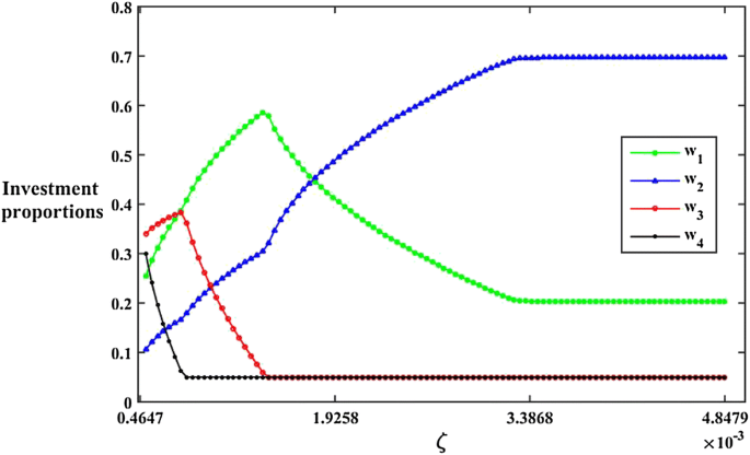

  

  Investment proportions under different values of $\zeta$ when $\beta = 0.5$ and $\alpha = 0.5$

• (3) When $\zeta > 0.0034$, the value of $R$ in Fig. 6 and the investment proportions in Fig. 7 are unchanged. According to Property 3, Model 5 will be the same as Model 3 if $\zeta = V_{\text{max} }$. Therefore, the investment proportions of Model 3 are the same as those of Model 5 for risk-seeking investors.

• (4) When the value of $\zeta$ increases, the values of $R$ and $w_{2}$ both increase. Moreover, the investment proportions are unchanged and the stock $a_{2}$ makes up a large proportion of investment when $\zeta > 0.0034$ (see Fig. 7). That is because the return of the stock $a_{2}$ is the highest when $\alpha = 0.5$(see Table 8), and the risk of the stock $a_{2}$ is also the highest when $\beta = 0.5$ (see Fig. 5). It is well known that high-return stocks usually have high risks. Risk-seeking investors are less sensitive to risks, so it is reasonable for them to choose the stocks with higher risks for higher returns.

In conclusion, the efficient frontier of our proposed Model 5 is reasonable. In the next section, we compare Model 5 with other portfolio selection models to highlight its superiority.

7.4 Comparison Between Model 5 and the Hesitant Fuzzy Portfolio Selection Model

As mentioned above, the DHFS is a good improvement of the HFS. Therefore, Model 5 is compared with the hesitant fuzzy portfolio selection model (HFPSM) proposed by Zhou and Xu [13] to show the superiority of Model 5.

7.4.1 Theoretical Comparison Between Model 5 and the HFPSM

According to the mathematical symbol of the hesitant fuzzy element (HFE) proposed by Xia and Xu [39], the set $H$ in $D_{R} = \left\langle {H,G} \right\rangle$ in Eq. (21) can be seen as a HFE. Moreover, based on the score function [39] of the HFE, the score function of $H$ is equivalent to $S_{H} (W)$ based on Eq. (23). According to the deviation function [40] of the HFE, the deviation function of $H$ is

$$ \overline{{V_{H} }} (W) = \frac{1}{{l_{H} }}\sum\limits_{u = 1}^{{l_{H} }} {\sqrt {(s_{u} (W) - S_{H} (W))^{2} } } . $$

(43)

In the hesitant fuzzy portfolio selection model [13], the score and deviation of the HFE are used to measure returns and risks, respectively. Therefore, the HFPSM for risk investors [13] is represented as follows.

HFPSM

$$ \begin{aligned} & { \text{max} }F(W) = S_{H} (W) \hfill \\ & {\text{s}} . {\text{t}}\left\{ \begin{aligned} & \overline{{V_{H} }} (W) \le \zeta \hfill \\ & \sum\limits_{i = 1}^{m} {w_{i} } = 1 \hfill \\ & w_{i} \ge 0,i = 1,2, \ldots ,m \hfill \\ \end{aligned} \right., \hfill \\ \end{aligned} $$

(44)

where $F(W)$ describes the portfolio return and $\zeta$ describes the investor’s risk appetite. $\zeta \in [V_{\text{min} } ,V_{\text{max} } ]$, where

$$ \begin{aligned} & V_{\text{max} } = \text{max} \, \overline{{V_{H} }} (W) \hfill \\ & {\text{s}} . {\text{t}}\left\{ \begin{aligned} & \sum\limits_{i = 1}^{m} {w_{i} } = 1 \hfill \\ & w_{i} \ge 0,i = 1,2, \ldots ,m \hfill \\ \end{aligned} \right. \hfill \\ \end{aligned} $$

(45)

and

$$ \begin{aligned} & V_{\text{min} } = \text{min} \, \overline{{V_{H} }} (W) \hfill \\ & {\text{s}} . {\text{t}} .\left\{ \begin{aligned} & \sum\limits_{i = 1}^{m} {w_{i} } = 1 \hfill \\ & w_{i} \ge 0,i = 1,2, \ldots ,m \hfill \\ \end{aligned} \right. \hfill \\ \end{aligned} . $$

(46)

According to Zhou and Xu [13]: if the investor is risk-seeking, then $\zeta = V_{\text{max} }$; if the investor is risk-neutral, then $\zeta = V_{\text{min} } + \frac{2}{3}(V_{\text{max} } - V_{\text{min} } )$; if the investor is risk-averse, then $\zeta = V_{\text{min} } + \frac{1}{3}(V_{\text{max} } - V_{\text{min} } )$. By comparing Model 5 and the HFPSM, we can obtain that:

• (1) Model 5 and the HFPSM both consider returns and risks, which are both applicable for investors with different risk appetites. When $\beta = 1$ and $\alpha = 1$, Model 5 is similar to the HFPSM.

• (2) Mode 5 considers information preference, which is not considered in the HFPSM. That is because Model 5 is constructed based on the DHFS, which can describe positive and negative information more comprehensively than the HFS. Therefore, Model 5 has a wider application than the HFPSM.

• (3) In the HFPSM, there are only three values of $\zeta$ for investors to choose. However, according to Property 3, the range $[V_{\text{min} } ,V_{\text{max} } ]$ in Model 5 is divided into three intervals, which include all the values of $\zeta$. Investors usually determine different values of $\zeta$ based on their risk appetites, so the setting of $\zeta$ in Model 5 is more reasonable.

7.4.2 Empirical Comparison Between Model 5 and the HFPSM

In this section, we compare Model 5 and the HFPSM based on the information and settings of parameters in case study. For convenience, we take the membership degrees of DHFEs in Tables 2 and 4 as the membership degrees of HFEs. Firstly, the investment proportions of the HFPSM and Model 5 under different risk appetites when $\alpha = 0.5$ and $\beta = 0.5$ are presented in Table 9. The following conclusions are obtained from Table 9.

Table 9 Investment proportions under different risk appetites in Model 5 and the HFPSM

• (1) For risk-averse investors, $w_{1}$ is the highest in the HFPSM, because the mean of membership degrees of the stock $a_{1}$ is the highest (see Table 7). In Model 5, $w_{1}$ is smaller than that in the HFPSM, while $w_{2}$ is larger than that in the HFPSM. The reason for this difference is that Model 5 considers the negative information of stocks. In Table 7, the mean of non-membership degrees of the stock $a_{1}$ is higher than that of the stock $a_{2}$, so $w_{1}$ decreases while $w_{2}$ increases.

• (2) For risk-neutral investors and risk-seeking investors in Model 5, $w_{2}$ increases while $w_{1}$ decreases, which is similar to that in conclusion (1). Moreover, the stock $a_{2}$ makes up a large proportion of investment for risk-seeking investors in Model 5, which can be explained by the highest return of the stock $a_{2}$ (see Table 8).

• (3) For risk-neutral investors and risk-seeking investors in the HFPSM, the stock $a_{1}$ makes up a main proportion of investment, which is different from that in conclusion (2). This is because the HFPSM only considers membership degrees and the mean of membership degrees of the stock $a_{1}$ is the highest (see Table 7). It is reasonable that investors who aim to make more profits will prefer the stocks with higher mean values of membership degrees in the HFPSM.

In conclusion, Model 5 can help investors with different information preferences find the optimal portfolios, which cannot be achieved by the HFPSM. Therefore, our proposed Model 5 is a good improvement of the HFPSM.

7.5 Utilities of the Proposed Models

According to the analyses above, the utilities of Model 3 and Model 5 are summarized as follows.

• (1) The proposed models can help investors to find the optimal portfolios when precise data are difficult to obtain. Model 3 is applicable for investors focusing on returns regardless of risks, whereas Model 5 is applicable for investors considering both returns and risks.

• (2) The parameter $\alpha$ in Model 3 and Model 5 can reflect investors’ information preferences in terms of returns. Moreover, the change of $\alpha$ is consistent with investors’ preferences for stocks, and higher values of $\alpha$ are more applicable for risk-seeking investors.

• (3) The parameter $\beta$ in Model 5 can reflect investors’ information preferences in terms of risks. In addition, lower values of $\beta$ are more applicable for risk-averse investors. However, the impact of $\beta$ on investment proportions depends on the return of each stock because the objective of Model 5 is to maximize the portfolio return.

• (4) The parameter $\zeta$ in Model 5 can describe investors’ risk appetites. The higher the value of $\zeta$, the higher the corresponding portfolio return. Therefore, Model 5 is applicable for risk-averse investors, risk-neutral investors and risk-seeking investors.

• (5) Compared with the hesitant fuzzy portfolio selection model, Model 5 can offer more options to the investors with different information preferences.

8 Conclusions

DHFS can validly describe uncertain information. Although there have been some decision-making models based on the DHFS, most of the research merely focuses on ranking the alternatives and choosing the best one. If the investment information is described by DHFSs and investors hope to find the optimal portfolios, the existing models are inapplicable. Therefore, we propose some novel portfolio selection models under dual hesitant fuzzy environment to solve this problem. The main contributions of this paper are concluded as follows.

• (1) To make use of positive and negative information in the DHFS, the parameter $\alpha$ is defined in Model 3 and Model 5 to capture investors’ information preferences in terms of returns, and the parameter $\beta$ is defined in Model 5 to capture investors’ information preferences in terms of risks.

• (2) The Max-score dual hesitant fuzzy portfolio selection model with information preference (Model 3) is proposed to help the investors focusing on returns regardless of risks to find the optimal portfolios. Moreover, it is proved that Model 3 is equivalent to a convex programming.

• (3) To consider the risks of portfolios, the score-deviation dual hesitant fuzzy portfolio selection model with information preference and risk appetite (Model 5) is developed. In Model 5, another parameter $\zeta$ is defined to capture investors’ risk appetites.

• (4) The sensitivity analysis, efficient frontier analysis and comparison analysis with the hesitant fuzzy portfolio selection model are conducted to highlight the utilities of the proposed models and the impacts of the parameters.

However, there are some limitations of the models. For example, the relationship among the parameters in Model 5 may have influence on the investment proportions, but the theoretical analysis on the relationship is not carried out in this paper because of the complexity. This is also one of the topics in our future study. Research on portfolio selection under dual hesitant fuzzy environment is still at an early stage. There is a lot of work to do in the future and we will keep on researching the portfolio selection in this area.

References

Markowitz, H.: Portfolio Selection. J. Financ. 7(1), 77–91 (1952)
Sharpe, W.F.: A simplified model for portfolio analysis. Manag. Sci. 9(2), 277–293 (1963)
Mao, J.C.T.: Models of capital budgeting, E-V VS E-S. J. Financ. Quant. Anal. 4(5), 657–675 (1970)
Best, M.J., Hlouskova, J.: The efficient frontier for bounded assets. Math. Methods Oper. Res. 52(2), 195–212 (2000)
Basak, S., Shapiro, A.: Value-at-risk-based risk management: optimal policies and asset prices. Rev. Financ. Stud. 14(2), 371–405 (2001)
Zadeh, L.A.: Fuzzy sets. Inf. Control 8(3), 338–353 (1965)
Dubois, D., Prade, H.M.: Fuzzy sets and systems: theory and applications. Academic Press, New York (1980)
Atanassov, K.T.: Intuitionistic fuzzy sets. Fuzzy Sets Syst. 20(1), 87–96 (1986)
Torra, V.: Hesitant fuzzy sets. Int. J. Intell. Syst. 25(6), 529–539 (2010)
Watada, J.: Fuzzy portfolio selection and its applications to decision making. Tatra Mt. Math. Publ. 13, 219–248 (1997)
Tanaka, H., Guo, P.J.: Portfolio selection based on upper and lower exponential possibility distributions. Eur. J. Oper. Res. 114(1), 115–126 (1999)
Deng, X., Pan, X.Q.: The research and comparison of multi-objective portfolio based on intuitionistic fuzzy optimization. Comput. Ind. Eng. 124, 411–421 (2018)
Zhou, W., Xu, Z.S.: Portfolio selection and risk investment under the hesitant fuzzy environment. Knowl. Based Syst. 144, 21–31 (2018)
Zhou, X.Y., et al.: A prospect theory-based group decision approach considering consensus for portfolio selection with hesitant fuzzy information. Knowl. Based Syst. 168, 28–38 (2019)
Zhu, B., Xu, Z.S., Xia, M.M.: Dual hesitant fuzzy sets. J. Appl. Math. 2012, 1–13 (2012)
Wang, L., Shen, Q.G., Zhu, L.: Dual hesitant fuzzy power aggregation operators based on Archimedean t-conorm and t-norm and their application to multiple attribute group decision making. Appl. Soft Comput. 38, 23–50 (2016)
Su, Z., et al.: Distance and similarity measures for dual hesitant fuzzy sets and their applications in pattern recognition. J. Intell. Fuzzy Syst. 29(2), 731–745 (2015)
Tyagi, S.K.: Correlation coefficient of dual hesitant fuzzy sets and its applications. Appl. Math. Model. 39(22), 7082–7092 (2015)
Zhao, N., Xu, Z.S.: Entropy measures for dual hesitant fuzzy information. (2015) https://doi.org/10.1109/csnt.2015.266
Hao, Z.N., et al.: Probabilistic dual hesitant fuzzy set and its application in risk evaluation. Knowl. Based Syst. 127, 16–28 (2017)
Zhang, H.D., et al.: Dual hesitant fuzzy rough set and its application. Soft. Comput. 21(12), 3287–3305 (2017)
Xu, X.R., Wei, G.W.: Dual hesitant bipolar fuzzy aggregation operators in multiple attribute decision making. Int. J. Knowl.-Based Intell. Eng. Syst. 21(3), 155–164 (2017)
Singh, P.: A new method for solving dual hesitant fuzzy assignment problems with restrictions based on similarity measure. Appl. Soft Comput. J. 24, 559–571 (2014)
Ren, Z.L., Wei, C.P.: A multi-attribute decision-making method with prioritization relationship and dual hesitant fuzzy decision information. Int. J. Mach. Learn. Cybern. 8(3), 755–763 (2017)
Ren, Z.L., Xu, Z.S., Wang, H.: Multi-criteria group decision-making based on quasi-order for dual hesitant fuzzy sets and professional degrees of decision makers. Appl. Soft Comput. J. 71, 20–35 (2018)
Tang, X.A., Yang, S.L., Pedrycz, W.: Multiple attribute decision-making approach based on dual hesitant fuzzy Frank aggregation operators. Appl. Soft Comput. J. 68, 525–547 (2018)
Yang, S.H., Ju, Y.B.: A GRA method for investment alternative selection under dual hesitant fuzzy environment with incomplete weight information. J. Intell. Fuzzy Syst. 28(4), 1533–1543 (2015)
Singh, P.: Distance and similarity measures for multiple-attribute decision making with dual hesitant fuzzy sets. Comput. Appl. Math. 36(1), 111–126 (2017)
Zhou, W., Xu, Z.S.: Score-hesitation trade-off and portfolio selection under intuitionistic fuzzy environment. Int. J. Intell. Syst. 34(2), 325–341 (2019)
Chang, D.Y.: Applications of the extent analysis method on fuzzy AHP. Eur. J. Oper. Res. 95(3), 649–655 (1996)
Wu, J.Z., Zhang, Q.: Multi criteria decision making method based on intuitionistic fuzzy weighted entropy. Expert Syst. Appl. 38(1), 916–922 (2011)
Chen, T.Y., Li, C.H.: Determining objective weights with intuitionistic fuzzy entropy measures: a comparative analysis. Inf. Sci. 180(21), 4207–4222 (2010)
Park, J.H., Kwark, H.E., Kwun, Y.C.: Entropy and cross-entropy for generalized hesitant fuzzy information and their use in multiple attribute decision making: entropy and cross-entropy For GHFISs. Int. J. Intell. Syst. 32(3), 266–290 (2017)
Chen, Y.F., et al.: Approaches to multiple attribute decision making based on the correlation coefficient with dual hesitant fuzzy information. J. Intell. Fuzzy Syst. 26(5), 2547–2556 (2014)
Su, Z., et al.: Distribution-based approaches to deriving weights from dual hesitant fuzzy information. Symmetry 11(1), 85 (2019)
Chen, H.P., Xu, G.Q., Yang, P.L.: Multi-attribute decision-making approach based on dual hesitant fuzzy information measures and their applications. Mathematics 7(9), 786 (2019)
Chen, J.J., Huang, X.J., Tang, J.: Distance measures for higher order dual hesitant fuzzy sets. Comput. Appl. Math. 37(2), 1784–1806 (2018)
Bertsekas, D.P.: Nonlinear programming, 2nd edn. Athena Scientific, Belmont (1999)
Xia, M.M., Xu, Z.S.: Hesitant fuzzy information aggregation in decision making. Int. J. Approx. Reason. 52(3), 395–407 (2011)
Zhou, W., Xu, Z.S.: Optimal discrete fitting aggregation approach with hesitant fuzzy information. Knowl. Based Syst. 78(1), 22–33 (2015)
Acknowledgements
This research was supported by the “Humanities and Social Sciences Research and Planning Fund of the Ministry of Education of China, No. x2lxY9180090”, “Natural Science Foundation of Guangdong Province, No. 2019A1515011038”, “Soft Science of Guangdong Province, and Nos. 2018A070712002, 2019A101002118”, and “Fundamental Research Funds for the Central Universities of China, No. x2lxC2180170”. The authors are highly grateful to the referees and editor in-chief for their very helpful comments.
Author information
Authors and Affiliations
Corresponding author
Rights and permissions
About this article
Cite this article
Li, W., Deng, X. Multi-parameter Portfolio Selection Model with Some Novel Score-Deviation Under Dual Hesitant Fuzzy Environment. Int. J. Fuzzy Syst. 22, 1123–1141 (2020). https://doi.org/10.1007/s40815-020-00835-8
Received:
Revised:
Accepted:
Published:
Issue Date:
DOI: https://doi.org/10.1007/s40815-020-00835-8