A Fuzzy Inventory Model for a Deteriorating Item with Variable Demand, Permissible Delay in Payments and Partial Backlogging with Shortage Follows Inventory (SFI) Policy

Abstract

This research studies a fuzzy inventory model for a deteriorating item with permissible delay in payments. For this paper, the demand depends on selling price and the frequency of the advertisement. In order to make a more realistic inventory model, it is considered the case of stock-out which is partial backlogged. In this work, it is taken account the shortage follows inventory (SFI) policy. Several scenarios and sub-scenarios have been provided, and each corresponding problem has been defined as a constrained optimization problem in the fuzzy environment. Further, these problems have converted into a new problem using the nearest interval approximation technique of fuzzy numbers. Quantum-behaved particle swarm optimization (QPSO) algorithm with the help of interval mathematics has been used to solve the optimization problems. Numerical examples have been solved in order to illustrate the proposed inventory model. Finally, with the aim to analyse the significant influence of different factors on the optimal policies, a sensitivity analysis is done.

1 Introduction and Literature Review

1.1 Motivation

Inventory management is essential for the smooth functioning of any firm. On the one hand, too much of inventory may lead to an addition of a high cost to the company. On the other hand, holding very few inventories may lead to stock-out situations and result in loss of potential customers. Inventory theory provides a solution to such problems by addressing the fundamental questions of when and how much to order. One of the basic models of inventory theory is the economic order quantity (EOQ) inventory model, which was derived by Harris [1] in 1913. Several studies have been done in the past on inventory management. Inventories are primarily classified as two types: perishable and non-perishable. Non-perishable items have a very long lifetime and hence can be used for demand fulfilment over a long period. Products that degrade in quality and utility with time are called perishable products. Perishable products are primarily of two categories: one, which maintains constant utility throughout the lifetime, for example medicines; while the other with exponentially decaying utility, for example, vegetables, fruits and fish [2]. Management of perishable items with limited lifetime is a challenge. The assure and care of deteriorating items of production inventories has obtained much attention of various investigators in the recent years as most tangible goods deteriorate through time. Because in reality, some of the goods either discredited or decomposed when the environment of products is changing due to weather conditions, pollution, etc. The effect of deterioration is increasing rapidly in manufacturing goods in various fields like food items, products related to pharmaceuticals and many others. Some part of such physical goods either got damaged or spoiled or evaporated or perished or affected due to many factors. Thus, the goods become not as good as they used to be and these cannot be supplied to customers to fulfil their demand. Therefore, the damage due to the deterioration phenomenon is very important to consider in the formulation of an inventory model.

The effect of globalization brings a high competition in the market that makes producers to hold inventory in such way so that they can capture more and more customers and the permissible delay in payment policy plays an important role in the businesses. Nowadays, suppliers provide different schemes and facilities to their retailers so that business can make smooth in nature. For example, one policy is to provide goods on credit under defined terms and conditions. Creditors pay no charge under the defined period of time but once the time got elapsed then they have to pay an extra payment in the form of the charge. This inventory problem is called as trade credit inventory or permissible delay in payments problem. Trade credit generates the following two benefits to the seller as stated in Chen et al. [3]: (a) it reduces the buyer’s cost and attracts new customers, and (b) it avoids permanent price competition. Trade credit enables separating flows of money from the flows of goods, which can be highly volatile or seasonal.

Haley and Higgins [4] first solved this class of inventory problem. Afterwards, Goyal [5] derived an EOQ inventory model considering conditions of permissible delay in payments. Subsequently, Aggarwal and Jaggi [6] revisited and extended the Goyal’s [5] inventory model for a deteriorating item. Their inventory model does not consider shortages. Jamal et al. [7] built a general EOQ inventory model, which considers fully backlogged shortages. It is important to remark that very few studies have addressed an inventory model for deteriorating items taking into consideration permissible delay in payment with shortage follow inventory policy. This has motivated us to develop a fuzzy inventory model for a deteriorating item with variable demand, permissible delay in payments and partial backlogging with shortage follows inventory (SFI) policy.

Haley and Higgins [4] first solved this kind of inventory problem. Later, Goyal [5] derived an EOQ inventory model under the conditions of permissible delay in payments. Subsequently, Aggarwal and Jaggi [6] revisited and extended the Goyal’s [5] inventory model for a deteriorating item. Their inventory model does not consider shortages. Jamal et al. [7] built a general EOQ inventory model, which considers fully backlogged shortages. It is important to note that very few studies have addressed a fuzzy inventory model considering deterioration with trade credit by shortage follows inventory (SFI) policy. This has motivated us to develop an inventory model considering the SFI policy.

1.2 Literature Review

1.2.1 Deteriorating Items

The first inventory model for deteriorating items was developed by Ghare and Schrader [2]. Afterwards, Emmons [8] built an inventory model for variable deterioration rate. After this, many researchers have extended the previous works in this field such as Covert and Philip [9], Giri et al. [10] and Ghosh and Chaudhuri [11], Chakrabarty et al. [12], Giri et al. [13], Sana et al. [14], Sana and Chaudhuri [15] and many more. Misra [16] derived an EOQ inventory model taking into account Weibull deterioration rate for a perishable item without considering backorders. In the same line of research, there are the works of Deb and Chaudhuri [17], Giri et al. [18], Goswami and Chaudhuri [19], Bhunia and Maiti [20, 21], Mandal and Phaujdar [22], Padmanabhan and Vrat [23], Pal et al. [24], Mandal and Maiti [25], Goyal and Gunasekaran [26], Sarker et al. [27], Pal et al. [28], amongst others. The reader may be directed to literature reviews on perishable inventory systems by Raafat et al. [29], Goyal and Giri [30], Bakker et al. [31], and Janssen et al. [32].

1.2.2 Trade Credit in Inventory

The real and favourable advantage of delayed payments is that suppliers give capital access and in this manner empower their clients to expand order sizes without moving towards a liquidity bottleneck. Likewise, they help to increase the competitive position of the suppliers who can utilize payments delays rather than value rebates to enhance sales and build up market position of their items [33]. Different empowering influences that encouraging the supply of trade credits are contrasts in the price elasticity amongst supplier and purchasers, credit intermediation amongst purchasers and banks and the insurance of non-salvageable interests in purchasers [34]. Thus, in numerous businesses, trade credits have turned out to be a standout amongst the most essential sources of short-term financing.

Goyal [5] demonstrated that the order quantity increases if predefined payment delays are allowed, when contrasted with the traditional EOQ inventory model. Teng [35] additionally expanded the inventory model of Goyal [5] and exhibited that in specific cases, it is useful for the purchaser to diminish its order quantity if trade credits are offered, and to profit by the admissible delay in payments by ordering more as often as possible.

1.2.3 Trade Credit and Fuzzy Inventory Model

The parameters in the previous mentioned studies related to inventory models are assumed to be known and constant. Regardless, at least one parameter of the inventory model frequently varies from cycle to cycle and displays a degree of uncertainty over the planning horizon. Within the sight of different vulnerabilities, it is tricky for retailers and merchandisers to have an accurate measure of demand. Moreover, most of the time, adequate historical information is not accessible to the inventory decision-maker or statistical inferences are incredible. Each situation raises challenges for applying traditional inventory models in real practice. To cope with uncertain accessible data in decision-making, it is ideal to describe inventory parameters using a fuzzy number. In addition, interest income and interest payments are two imperative issues that concern trade credit. Because of economic globalization and advancement, the interest rate is probably not going to stay stable consistently. In this way, it is advantageous to describe the interest rate as a fuzzy number. Das et al. [36, 37] and Guchhait et al. [38, 39] investigated the inventory model under fuzzy trade credit with decaying items considering various scenarios. They assumed two types of deterioration for finished product and raw material as well. Several inventory models have been proposed by academicians and researchers. These inventory models include different types of considerations with respect to deterioration, demand, shortage policy, level of permissible delay in payments, inventory policy, amongst others characteristics. The details of some research works are presented in Table 1.

Table 1 Related literature for trade credit inventory models

Recently, Bhunia et al. [56] studied an inventory pricing model for a deteriorating product considering demand depends on both stock and price discount. After that, Bhunia and Shaikh [57] introduced an inventory model by considering that inventory parameters are interval valued with both inventory follows shortage (IFS) and shortage follows inventory (SFI) policies. They solved this problem by particle swarm optimization technique. However, this inventory model does not consider permissible delay in payments.

The present paper contributes to the existing literature proposing an inventory model for a deteriorating item taking into account permissible delay in payments, demand dependent on selling price and advertisement’s frequency and shortage follows inventory (SFI) policy in a fuzzy environment.

2 Assumptions and Notation

The assumptions and notation that are needed to develop the inventory model are shown below.

2.1 Assumptions

• 1. The demand rate depends on selling price of the item and frequency of advertisement in different media. Here, the demand rate is given by $D(A,p) = A^{\gamma } (a - bp)$, where $a,b,\gamma > 0$ and with the condition $0 < p < \frac{a}{b}$.

• 2. The entire lot is supplied in one order.

• 3. Lead time is constant and known, and replenishment rate is infinite.

• 4. Deterioration occurs only after the lot is received. There is neither repair nor replacement of deteriorated items for the period of the replenishment cycle.

• 5. The planning horizon is infinite.

• 6. Supplier offers a fixed credit period to the retailer.

• 7. Shortages are permitted, and unsatisfied demand is partially backlogged. During the shortage period, the backlogging rate depends on the duration of the waiting time till the arrival of the next order. The backlogging rate is determined with $[1 + \delta (t_{s} - t)]^{ - 1} ,\delta > 0.$

2.2 Notation

Parameters
$C_{\text{o}} ,\tilde{C}_{\text{o}}$	Crisp and fuzzy ordering costs per order ($/order)
$C_{\text{p}} ,\tilde{C}_{\text{p}}$	Crisp and fuzzy purchasing costs of retailer per unit ($/unit)
$C_{\text{h}} ,\tilde{C}_{\text{h}}$	Crisp and fuzzy holding costs per unit per unit time ($/unit/time unit)
$C_{\text{b}} ,\tilde{C}_{\text{b}}$	Crisp and fuzzy shortage costs per unit per unit time ($/unit/time unit)
$C_{\text{ls}} ,\tilde{C}_{\text{ls}}$	Crisp and fuzzy opportunity costs per unit due to lost sale ($/unit)
$C_{\text{A}}$	Advertisement cost per advertisement ($/advertisement)
$I_{\text{e}}$	Interest earned by the retailer per unit time (%/time unit)
$I_{\text{p}}$	Interest payable to the supplier per unit time (%/time unit)
$p$	Selling price per unit ($/unit)
$\theta$	Constant deterioration rate ($0 < \theta \ll 1$)
$M$	Length of credit period offered by the supplier to his/her retailer(time unit)
$I(t)$	Inventory level at time t (units)
$D(A,p)$	Demand function (units/time unit)
$Z_{\text{p}} = [Z_{\text{pL}} ,Z_{\text{pR}} ]$	Total profit per unit of time of the inventory system ($/time unit)
Decision variables
$A$	Frequency of advertisement (an integer value)
$t_{\text{s}}$	Time when the shortage quantity achieves to the highest level R (time unit)
$t_{1}$	Time when inventory level attains to zero. Also, it represents the cycle length (time unit)
Dependent variables
$S$	Highest stock quantity at the starting of stock period (units)
$R$	Maximum shortage quantity (units)
$Q$	Lot size, $Q = S + R$, (units)

3 The Nearest Interval Approximation of a Fuzzy Number

A fuzzy number is a fuzzy set that is both convex and normal. This number plays a significant role to formulate the model of real-world decision-making problems with uncertain parameters. The basics of fuzzy sets and fuzzy numbers are described in the existing literature. This paper uses nearest interval approximations of fuzzy numbers such as triangular fuzzy number (TFN), Trapezoidal fuzzy number (TrFN) and parabolic fuzzy number (PFN).

Let $\tilde{A}$ be a fuzzy number with interval of confidence at the level $\alpha$; $[A_{\text{L}} (\alpha ),A_{\text{R}} (\alpha )]$. According to Grzegorzewski [58], the nearest interval approximation of fuzzy number $\tilde{A}$ is a crisp interval number which is represented by $\left[ {\int\limits_{0}^{1} {A_{\text{L}} (\alpha ){\text{d}}\alpha ,\int\limits_{0}^{1} {A_{\text{R}} (\alpha ){\text{d}}\alpha } } } \right]$. Applying this formula, interval approximations of three different fuzzy numbers are shown in Table 2.

Table 2 Interval approximations of three different fuzzy numbers

4 Mathematical Formulation of the Inventory Model Under Crisp Environment

Here, the inventory cycle starts with shortage and ends without shortage at time $t_{1}$ (see Fig. 1). In the beginning (i.e. at time $t = 0$), shortages start to accumulate with a rate $[1 + \delta (t_{\text{s}} - t)]^{ - 1} ,\delta > 0$ and continue till the time $t = t_{\text{s}}$. At time $t = t_{\text{s}}$, a lot of $(Q = S + R)$ units of the item is purchased and received. Then, the inventory level diminishes by reason of demand and deterioration, and it achieves to zero at $t = t_{1} .$

Fig. 1

Inventory level through time

The inventory level $I(t)$ at time $t$ is modelled by the according to differential equations:

$$\frac{{{\text{d}}I(t)}}{{{\text{d}}t}} = \frac{ - D(A,p)}{{\left\{ {1 + \delta \left( {t_{\text{s}} - t} \right)} \right\}}},\quad 0 \le t \le t_{\text{s}}$$

(1)

$$\frac{{{\text{d}}I(t)}}{{{\text{d}}t}} + \theta I(t) = - \,D(A,p),\quad t_{\text{s}} < t \le t_{1}$$

(2)

with the conditions

$$I(t) = - R\quad {\text{at}}\quad t = t_{\text{s}}^{ - } ,$$

(3)

and

$$I(t) = 0\quad {\text{at}}\quad t = t_{1} .$$

(4)

Using (3) and (4), thus the solutions of (1) and (2) are expressed by

$$I\left( t \right) = - \,R + {{D(A,p)\log \left| {1 + \delta \left( {t_{\text{s}} - t} \right)} \right|} \mathord{\left/ {\vphantom {{D(A,p)\log \left| {1 + \delta \left( {t_{\text{s}} - t} \right)} \right|} \delta }} \right. \kern-0pt} \delta },\quad 0 \le t \le t_{\text{s}}$$

(5)

$$I(t) = {{D(A,p)\left\{ {e^{{\theta (t_{1} - t)}} - 1} \right\}} \mathord{\left/ {\vphantom {{D(A,p)\left\{ {e^{{\theta (t_{1} - t)}} - 1} \right\}} \theta }} \right. \kern-0pt} \theta },\quad t_{\text{s}} < t \le t_{1}$$

(6)

$${\text{Moreover, }}I\left( t \right) = 0\;{\text{at}}\;t = 0\quad {\text{and}}\quad I\left( t \right) = S\;{\text{at}}\;t = t_{\text{s}} .$$

(7)

Therefore,

$$S = {{D(A,p)\left\{ {e^{{\theta (t_{1} - t_{\text{s}} )}} - 1} \right\}} \mathord{\left/ {\vphantom {{D(A,p)\left\{ {e^{{\theta (t_{1} - t_{\text{s}} )}} - 1} \right\}} \theta }} \right. \kern-0pt} \theta }$$

(8)

The total holding cost $(C_{\text{hol}} )$ is calculated by

$$C_{\text{hol}} = C_{\text{h}} \int\limits_{{t_{\text{s}} }}^{{t_{1} }} {I(t){\text{d}}t}$$

(9)

From $I(t) = 0$ at $t = 0$, then the shortage level is determined with

$$R = {{D(A,p)\log \left| {1 + \delta t_{\text{s}} } \right|} \mathord{\left/ {\vphantom {{D(A,p)\log \left| {1 + \delta t_{\text{s}} } \right|} \delta }} \right. \kern-0pt} \delta }$$

(10)

The total shortage cost ($C_{\text{sho}}$) for the duration of the whole inventory cycle is expressed by

$$C_{\text{sho}} = C_{\text{b}} \int\limits_{0}^{{t_{\text{s}} }} {\left[ { - I\left( t \right)} \right]{\text{d}}t}$$

(11)

The total cost of lost sale (${\text{OCLS}}$) for the period of the inventory cycle is obtained with

$${\text{OCLS}} = C_{\text{ls}} \int\limits_{0}^{{t_{\text{s}} }} {D(A,p)} \left\{ {1 - \frac{1}{{1 + \delta \left( {t_{\text{s}} - t} \right)}}} \right\}{\text{d}}t$$

(12)

Advertisement cost ($C_{\text{adv}}$) during the inventory cycle is computed by

$$C_{\text{adv}} = C_{\text{A}} A$$

As M is the fixed trade credit period provided by the supplier to the retailer then there exist two scenarios as follows: Scenario 4.1 $t_{\text{s}} < M \le t_{1}$ and Scenario 4.2 $t_{1} \le M$.

Now, these two scenarios are discussed in detail below.

Scenario 4.1

$t_{\text{s}} < M \le t_{1}$. In this case, the total sales revenue during $[t_{\text{s}} ,M]$ is determined with $p\int\limits_{{t_{s} }}^{M} {D(A,p){\text{d}}t}$ and the interest earned on that sales revenue from $t_{\text{s}}$ to $M$ is calculated with $pI_{\text{e}} \int\limits_{{t_{\text{s}} }}^{M} {\int\limits_{{t_{s} }}^{t} {D(A,p){\text{d}}u{\text{d}}t} }$. At time $t = M$, the retailer has accumulated the amount:

$$\begin{aligned} U_{1} & = p\int\limits_{{t_{\text{s}} }}^{M} {D(A,p){\text{d}}t} + pI_{\text{e}} \int\limits_{{t_{\text{s}} }}^{M} {\int\limits_{{t_{\text{s}} }}^{t} {D(A,p){\text{d}}u{\text{d}}t} } \\ & \quad + pR\left\{ {1 + I_{\text{e}} (M - t_{\text{s}} )} \right\} \\ \end{aligned}$$

On the other hand, the retailer must pay $C_{\text{p}} (S + R)$ amount to the supplier. Here, the following two sub-scenarios arise: Sub-scenario 4.1.1 $U_{1} < C_{\text{p}} (S + R)$ and Sub-scenario 4.1.2 $U_{1} \ge C_{\text{p}} (S + R)$. These two sub-scenarios are explained below.

Sub-scenario 4.1.1

$U_{1} < C_{\text{p}} (S + R)$ In this sub-scenario, the retailer’s earning amount is not enough to the payable amount of the supplier. In that case, supplier may agree to take the partial payment or not. Considering these situations, two cases occur: Case 4.1.1.1 When partial payment is allowed at time $t = M$ and Case 4.1.1.2 When partial payment is not permitted at time $t = M$. These two cases are described below.

Case 4.1.1.1

When partial payment is allowed at time $t = M.$ In this case, at time $t = M,$ the retailer must pay $U_{1}$ amount to the supplier and the rest amount $\left\{ {C_{\text{p}} (S + R) - U_{1} } \right\}$ along with the interest charged must be paid at time $t = B(B > M)$. Therefore, at time $t = B$, the total payable amount is $\left\{ {C_{\text{p}} (S + R) - U_{1} } \right\}\left\{ {1 + I_{\text{p}} \left( {B - M} \right)} \right\}$. During the time period $[M,B]$, the retailer also earns the interest on the sales revenue. The interest earned from M to B is obtained with $pI_{\text{e}} \int\limits_{M}^{B} {\int\limits_{M}^{t} {D(A,p){\text{d}}u{\text{d}}t} }$ and the total sales revenue for the time period $[M,B]$ is computed with $p\int\limits_{M}^{B} {D(A,p){\text{d}}t}$. Now, the total available amount to the retailer is given by

$$\begin{aligned} & \left\langle {{\text{selling}}\;{\text{amount}}\;{\text{during}}\;[M,B]} \right\rangle \\ & \quad + \left\langle {{\text{the}}\;{\text{interest}}\;{\text{earned}}\;{\text{on}}\;{\text{that}}\;{\text{selling}}\;{\text{amount}}} \right\rangle \\ & \quad = p\int\limits_{M}^{B} {D(A,p){\text{d}}t} + pI_{\text{e}} \int\limits_{M}^{B} {\int\limits_{M}^{t} {D(A,p){\text{d}}u{\text{d}}t} } . \\ \end{aligned}$$

(13)

Thus, at time $t = B$, the amount payable to the supplier is equal to the total amount available to the retailer which is given by

$$\begin{aligned} & \left\{ {C_{\text{p}} (S + R) - U_{1} } \right\}\left\{ {1 + I_{\text{p}} \left( {B - M} \right)} \right\} \\ & \quad = \, p\int\limits_{M}^{B} {D(A,p){\text{d}}t} + pI_{\text{e}} \int\limits_{M}^{B} {\int\limits_{M}^{t} {D(A,p){\text{d}}u{\text{d}}t} } \\ \end{aligned}$$

(14)

From Eq. (14), B can be expressed explicitly in terms of other parameters.

Now, the total sales revenue during the time period $[B,t_{1} ]$ is $p\int\limits_{B}^{{t_{1} }} {D(A,p)dt}$ and the interest earned during the time period $[B,t_{1} ]$ is $pI_{e} \int\limits_{B}^{{t_{1} }} {\int\limits_{B}^{t} {D(A,p){\text{d}}u{\text{d}}t} } .$

Therefore, the total profit per unit of time for the cycle is expressed mathematically by

$$Z_{\text{p}}^{{\left( {4.1.1.1} \right)}} \left( {A,t_{\text{s}} ,t_{1} } \right) = \frac{{X_{1} }}{{t_{1} }}$$

(15)

where

$$\begin{aligned} X_{1} & = \left\langle {{\text{total}}\;{\text{sales}}\;{\text{revenue}}\;{\text{during}}\; [B,t_{1} ]} \right\rangle \\ & \quad + \left\langle {{\text{interest}}\;{\text{earned}}\;{\text{during}}\; [B,t_{1} ] } \right\rangle - \left\langle {{\text{ordering}}\;{\text{cost}}} \right\rangle \\ & \quad {-}\left\langle {{\text{holding}}\;{\text{cost}}} \right\rangle - \left\langle {{\text{shortage}}\;{\text{cost}}} \right\rangle \\ & \quad {-}\left\langle {{\text{cost}}\;{\text{of}}\;{\text{lost}}\;{\text{sales}}} \right\rangle - \left\langle {{\text{advertisement}}\;{\text{cost}}} \right\rangle \\ \end{aligned}$$

$$\begin{aligned} X_{1} & = p\int\limits_{B}^{{t_{1} }} {D(A,p){\text{d}}t} + pI_{\text{e}} \int\limits_{B}^{{t_{1} }} {\int\limits_{B}^{t} {D(A,p){\text{d}}u{\text{d}}t} } \\ & \quad - C_{\text{o}} - C_{\text{hol}} - C_{\text{sho}} - {\text{OCLS}} - C_{\text{adv}} \\ \end{aligned}$$

(16)

Hereafter, the resultant constrained optimization problem is given by Problem 1 as follows:

Problem 1

$$\begin{array} {ll}{\text{Maximize}}\;Z_{\text{p}}^{{\left( {4.1.1.1} \right)}} \left( {A,t_{\text{s}} ,t_{1} } \right) = \frac{{X_{1} }}{{t_{1} }} \hfill \\ {\text{subject}}\;{\text{to}}\;t_{\text{s}} & M \le t_{1} \hfill \\ \end{array}$$

(17)

Case 4.1.1.2

When partial payment is not permitted at time $t = M.$ In this case, full payment is made after any time $t = M$. Let this time point be $B$. At time $t = M$, the retailer has $U_{1}$ amount available, so from this amount, he or she earns interest for the time period $[M,B]$, but he must pay the interest for the time period $[M,B]$.

The interest earned on $U_{1}$ from $M$ to $B$ is $U_{1} I_{\text{e}} (B - M)$. The interest earned on the sales revenue $M$ to $B$ is $pI_{\text{e}} \int\limits_{M}^{B} {\int\limits_{M}^{t} {D(A,p){\text{d}}u{\text{d}}t} }$ and the total sales revenue for the period $[M,B]$ is $p\int\limits_{M}^{B} {D(A,p){\text{d}}t}$.

Thus, the total amount earned by the retailer up to time $t = B$ is $U_{1} \{ 1 + I_{\text{e}} (B - M)\} + \left( {pI_{\text{e}} \int\limits_{M}^{B} {\int\limits_{M}^{t} {D(A,p){\text{d}}u{\text{d}}t} } + p\int\limits_{M}^{B} {D(A,p){\text{d}}t} } \right)$ and the payable amount to the supplier is $C_{\text{p}} (S + R)\{ 1 + I_{\text{p}} (B - M)\} .$

Clearly, the quantity payable to the supplier is equal to the total quantity available to the retailer at time $t = B.$ Therefore,

$$\begin{aligned} & C_{\text{p}} (S + R)\{ 1 + I_{\text{p}} (B - M)\} \\ & \quad = U_{1} \{ 1 + I_{\text{e}} (B - M)\} \\ & \quad \quad + pI_{\text{e}} \int\limits_{M}^{B} {\int\limits_{M}^{t} {D(A,p){\text{d}}u{\text{d}}t} } + p\int\limits_{M}^{B} {D(A,p){\text{d}}t} \\ \end{aligned}$$

(18)

from which B can be expressed explicitly in terms of other parameters.

Now, the total sales revenue during the time period $[B,t_{1} ]$ is calculated with $p\int\limits_{B}^{{t_{1} }} {D(A,p){\text{d}}t}$ and the interest earned during $[B,t_{1} ]$ is determined with $pI_{\text{e}} \int\limits_{B}^{{t_{1} }} {\int\limits_{B}^{t} {D(A,p){\text{d}}u{\text{d}}t} }$.

Consequently, the total profit per unit of time for the cycle is expressed as

$$Z_{\text{p}}^{(4.1.1.2)} \left( {A,t_{\text{s}} ,t_{1} } \right) = \frac{{X_{2} }}{{t_{1} }}$$

(19)

where

$$\begin{aligned} X_{2} & = \left\langle {{\text{total}}\;{\text{sales}}\;{\text{revenue}}\;{\text{during}}\; [B,t_{1} ]} \right\rangle \\ & \quad + \left\langle {{\text{interest}}\;{\text{earned}}\;{\text{during }}\; [B,t_{1} ]} \right\rangle - \left\langle {{\text{ordering}}\;{\text{cost}}} \right\rangle \\ & \quad {-}\,\left\langle {{\text{holding}}\;{\text{cost}}} \right\rangle - \left\langle {{\text{shortage}}\;{\text{cost}}} \right\rangle {-}\left\langle {{\text{cost}}\;{\text{of}}\;{\text{lost}}\;{\text{sales}}} \right\rangle - \left\langle {{\text{advertisement}}\;{\text{cost}}} \right\rangle \\ \end{aligned}$$

$$X_{2} = p\int\limits_{B}^{{t_{1} }} {D(A,p){\text{d}}t} + pI_{\text{e}} \int\limits_{B}^{{t_{1} }} {\int\limits_{B}^{t} {D(A,p){\text{d}}u{\text{d}}t} } - C_{\text{o}} - C_{\text{hol}} - C_{\text{sho}} - {\text{OCLS}} - C_{\text{adv}}$$

(20)

As a result, the resultant constrained optimization problem is stated by Problem 2 as follows:

Problem 2

$$\begin{aligned}& {\text{Maximize}}\;Z_{\text{p}}^{(4.1.1.2)} \left( {A,t_{\text{s}} ,t_{1} } \right) = \frac{{X_{2} }}{{t_{1} }} \hfill \\& {\text{subject}}\;{\text{to}}\;t_{\text{s}} < M \le t_{1} \hfill \\ \end{aligned}$$

(21)

Sub-scenario 4.1.2

$U_{1} \ge C_{\text{p}} (S + R)$

In this sub-scenario, at time $t = M$, retailer must pay only $C_{\text{p}} (S + R)$ amount to the supplier. So, he or she earns the interest for the time period $[M,t_{1} ]$ from the excess amount $\left\{ {U_{1} - C_{\text{p}} (S + R)} \right\}$. The retailer starts to accumulate the revenues continuously on the sales and earns interest on that revenue after time $t = M$.

Thus, the total sales revenue is

$$p\int\limits_{M}^{{t_{1} }} {D(A,p){\text{d}}t} .$$

(22)

The interest earned by the retailer is

$$pI_{\text{e}} \int\limits_{M}^{{t_{1} }} {\int\limits_{M}^{t} {D(A,p){\text{d}}u{\text{d}}t} .}$$

(23)

Then, the total profit per unit of time for the cycle is computed by

$$Z_{\text{p}}^{(4.1.2)} \left( {A,t_{\text{s}} ,t_{1} } \right) = \frac{{X_{3} }}{{t_{1} }}$$

(24)

where $\begin{aligned} X_{3} & = \left\langle {{\text{Excess}}\;{\text{amount}}\;{\text{after}}\;{\text{paying}}\;{\text{the}}\;{\text{amount}}\;{\text{to}}\;{\text{the}}\;{\text{supplier}}} \right\rangle + \left\langle {{\text{interest}}\;{\text{earned}}\;{\text{for}}\;{\text{the}}\;{\text{excess}}\;{\text{amount}}\;{\text{during}}\; [M,t_{1} ]} \right\rangle \\ & \quad + \left\langle {{\text{total}}\;{\text{sales}}\;{\text{revenue}}\;{\text{during}}\; [M,t_{1} ]} \right\rangle + \left\langle {{\text{interest}}\;{\text{earned}}\;{\text{during}}\;[M,t_{1} ]} \right\rangle - \left\langle {{\text{ordering}}\;{\text{cost}}} \right\rangle {-}\,\left\langle {{\text{holding}}\;{\text{cost}}} \right\rangle \\ & \quad - \left\langle {{\text{shortage}}\;{\text{cost}}} \right\rangle {-}\left\langle {{\text{cost}}\;{\text{of}}\;{\text{lost}}\;{\text{sales}}} \right\rangle - \left\langle {{\text{advertisement}}\;{\text{cost}}} \right\rangle \\ \end{aligned}$

$$\begin{aligned} X_{3} & = \left\{ {U_{1} - C_{\text{p}} (S + R)} \right\}\left\{ {1 + I_{\text{e}} \left( {t_{1} - M} \right)} \right\} + p\int\limits_{M}^{{t_{1} }} {D(A,p){\text{d}}t} + pI_{\text{e}} \int\limits_{M}^{{t_{1} }} {\int\limits_{M}^{t} {D(A,p){\text{d}}u{\text{d}}t} } \\ & \quad - C_{\text{o}} - C_{\text{hol}} - C_{\text{sho}} - {\text{OCLS}} - C_{\text{adv}} \\ \end{aligned}$$

(25)

So, the resultant constrained optimization problem is written in Problem 3 as follows:

Problem 3

$$\begin{aligned}& {\text{Maximize}}\;Z_{\text{p}}^{(4.1.2)} \left( {A,t_{\text{s}} ,t_{1} } \right) = \frac{{X_{3} }}{{t_{1} }} \hfill \\& {\text{subject}}\;{\text{to}}\;t_{\text{s}} < M \le t_{1} \hfill \\ \end{aligned}$$

(26)

Scenario 4.2

$t_{1} \le M$ In this scenario, the total sales revenue during the time period $[t_{\text{s}} ,t_{1} ]$ is determined with

$$p\int\limits_{{t_{\text{s}} }}^{{t_{1} }} {D(A,p){\text{d}}t} .$$

(27)

The interest earned during the time period $[t_{\text{s}} ,t_{1} ]$ is given by

$$pI_{\text{e}} \int\limits_{{t_{\text{s}} }}^{{t_{1} }} {\int\limits_{{t_{\text{s}} }}^{t} {D(A,p){\text{d}}u{\text{d}}t} }$$

(28)

and the interest earned during the time period $[t_{1} ,M]$ is calculated as

$$\left( {p\int\limits_{{t_{\text{s}} }}^{{t_{1} }} {D(A,p){\text{d}}t} + pI_{\text{e}} \int\limits_{{t_{\text{s}} }}^{{t_{1} }} {\int\limits_{{t_{\text{s}} }}^{t} {D(A,p){\text{d}}u{\text{d}}t} } } \right)I_{\text{e}} (M - t_{1} ).$$

(29)

Hence, the total revenue earned by the retailer is obtained with

$$U_{2} = \left\{ {p\int\limits_{{t_{\text{s}} }}^{{t_{1} }} {D(A,p){\text{d}}t} + pI_{\text{e}} \int\limits_{{t_{\text{s}} }}^{{t_{1} }} {\int\limits_{{t_{\text{s}} }}^{t} {D(A,p){\text{d}}u{\text{d}}t} } } \right\}\left\{ {1 + I_{\text{e}} \left( {M - t_{1} } \right)} \right\} + pR\left\{ {1 + I_{\text{e}} (M - t_{\text{s}} )} \right\}.$$

(30)

Therefore, the total profit per unit of time for the cycle is given by

$$Z_{\text{p}}^{(4.2)} \left( {A,t_{\text{s}} ,t_{1} } \right) = \frac{{X_{4} }}{{t_{1} }}$$

(31)

where

$$\begin{aligned} X_{4} & = \left\langle {\text{excess amount}} \right\rangle + \left\langle {{\text{interest}}\;{\text{earned}}\;{\text{for}}\;{\text{the}}\;{\text{excess}}\;{\text{amount}}} \right\rangle - \left\langle {{\text{ordering}}\;{\text{cost}}} \right\rangle \\ & \quad {-}\left\langle {{\text{holding}}\;{\text{cost}}} \right\rangle - \left\langle {{\text{shortage}}\;{\text{cost}}} \right\rangle {-}\left\langle {{\text{cost}}\;{\text{of}}\;{\text{lost}}\;{\text{sales}}} \right\rangle - \left\langle {{\text{advertisement}}\;{\text{cost}}} \right\rangle \\ \end{aligned}$$

$$X_{4} = U_{2} - C_{\text{p}} (S + R) - C_{\text{o}} - C_{\text{hol}} - C_{\text{sho}} - {\text{OCLS}} - C_{\text{adv}}$$

In this scenario, the resultant constrained optimization problem is expressed in Problem 4 as follows:

Problem 4

$$\begin{aligned} &{\text{Maximize}}\;Z_{\text{p}}^{(4.2)} \left( {A,t_{\text{s}} ,t_{1} } \right) = \frac{{X_{4} }}{{t_{1} }} \hfill \\& {\text{subject}}\;{\text{to}}\;t_{1} \le M \hfill \\ \end{aligned}$$

(32)

5 Fuzzy Inventory Model

In fuzzy environment, all the differential equations, their solutions and the expressions for S and R are the same as in the formulation of crisp environment.

The total holding cost $\tilde{C}_{\text{hol}}$ is given by $\tilde{C}_{\text{hol}} = \tilde{C}_{\text{h}} \int\limits_{{t_{\text{s}} }}^{{t_{1} }} {I(t){\text{d}}t}$

Here, the total shortage cost $\tilde{C}_{\text{sho}}$ through the complete inventory cycle is computed as

$$\tilde{C}_{\text{sho}} = \tilde{C}_{\text{b}} \int\limits_{0}^{{t_{\text{s}} }} {\left[ { - I\left( t \right)} \right]{\text{d}}t}$$

(33)

The total cost of lost sale ${\text{OCLS}}$ thru the inventory cycle is determined with

$${\text{OCLS}} = \tilde{C}_{\text{ls}} \int\limits_{0}^{{t_{\text{s}} }} {D(A,p)} \left\{ {1 - \frac{1}{{1 + \delta \left( {t_{\text{s}} - t} \right)}}} \right\}{\text{d}}t$$

(34)

Like in crisp inventory model, here two scenarios arise: Scenario 5.1 $t_{\text{s}} < M \le t_{1}$ and Scenario 5.2 $t_{1} \le M$. These two scenarios are explained below.

Scenario 5.1

$t_{\text{s}} < M \le t_{1}$ At time $t = M$, the retailer has accumulated the amount

$$U_{1} = p\int\limits_{{t_{\text{s}} }}^{M} {D(A,p){\text{d}}t} + pI_{\text{e}} \int\limits_{{t_{\text{s}} }}^{M} {\int\limits_{{t_{\text{s}} }}^{t} {D(A,p){\text{d}}u{\text{d}}t} } + pR\left\{ {1 + I_{\text{e}} (M - t_{\text{s}} )} \right\}$$

But, the retailer must pay $\tilde{C}_{\text{p}} (S + R)$ amount to the supplier. Thus, two sub-scenarios occur: Sub-scenario 5.1.1 $U_{1} < \tilde{C}_{\text{p}} (S + R)$ and Sub-scenario 5.1.2 $U_{1} \ge \tilde{C}_{\text{p}} (S + R)$. These two sub-scenarios are addressed below.

Sub-scenario 5.1.1

$U_{1} < \tilde{C}_{\text{p}} (S + R)$ Like crisp inventory model, in this sub-scenario, again two cases occur: Case 5.1.1.1 when partial payment is allowed at time $t = M$ and Case 5.1.1.2 when partial payment is not permitted at time $t = M.$

Case 5.1.1.1

When partial payment is allowed at time $t = M.$ In this case, the total profit per unit of time for the cycle is given by

$$Z_{\text{p}}^{(5.1.1.1)} \left( {A,t_{\text{s}} ,t_{1} } \right) = \frac{{\tilde{X}_{1} }}{{t_{1} }}$$

(35)

where

$$\begin{aligned} \tilde{X}_{1} & = \left\langle {{\text{total}}\;{\text{sales}}\;{\text{revenue}}\;{\text{during }}\left[ {{\text{B,t}}_{ 1} } \right]} \right\rangle + \left\langle {{\text{interest}}\;{\text{earned}}\;{\text{during}}\;[B,t_{1} ]} \right\rangle - \left\langle {{\text{ordering}}\;{\text{cost}}} \right\rangle \\ & \;{-}\left\langle {{\text{holding}}\;{\text{cost}}} \right\rangle - \left\langle {{\text{shortage}}\;{\text{cost}}} \right\rangle {-}\left\langle {{\text{cost}}\;{\text{of}}\;{\text{lost}}\;{\text{sales}}} \right\rangle - \left\langle {{\text{advertisement}}\;{\text{cost}}} \right\rangle \\ \end{aligned}$$

Thus, $\tilde{X}_{1} = p\int\limits_{{\tilde{B}}}^{{t_{1} }} {D(A,p){\text{d}}t} + pI_{\text{e}} \int\limits_{{\tilde{B}}}^{{t_{1} }} {\int\limits_{{\tilde{B}}}^{t} {D(A,p){\text{d}}u{\text{d}}t} } - \tilde{C}_{\text{o}} - \tilde{C}_{\text{hol}} - \tilde{C}_{\text{sho}} - {\text{OCLS}} - C_{\text{adv}}$

Then, the constrained optimization is expressed below:

Problem 5

$$\begin{aligned} &{\text{Maximize}}\,Z_{\text{p}}^{(5.1.1.1)} \left( {A,t_{\text{s}} ,t_{1} } \right) = \frac{{\tilde{X}_{1} }}{{t_{1} }} \hfill \\ &{\text{subject}}\;{\text{to}}\;t_{\text{s}} < M \le t_{1} \hfill \\ \end{aligned}$$

(36)

Case 5.1.1.2

When partial payment is not permitted at time $t = M$ In this case, the total profit per unit of time for the cycle is given by

$$Z_{\text{p}}^{(5.1.1.2)} \left( {A,t_{\text{s}} ,t_{1} } \right) = \frac{{\tilde{X}_{2} }}{{t_{1} }}$$

(37)

where

$$\begin{aligned} \tilde{X}_{2} & = \left\langle {{\text{total}}\;{\text{sales}}\;{\text{revenue}}\;{\text{during}}\;[B,t_{1} ] } \right\rangle + \left\langle {{\text{interest}}\;{\text{earned}}\;{\text{during}}\;[B,t_{1} ]} \right\rangle - \left\langle {{\text{ordering}}\;{\text{cost}}} \right\rangle \\ & \quad {-}\left\langle {{\text{holding}}\;{\text{cost}}} \right\rangle - \left\langle {{\text{shortage}}\;{\text{cost}}} \right\rangle {-}\left\langle {{\text{cost}}\;{\text{of}}\;{\text{lost}}\;{\text{sales}}} \right\rangle - \left\langle {{\text{advertisement}}\;{\text{cost}}} \right\rangle \\ \end{aligned}$$

$$\tilde{X}_{2} = p\int\limits_{B}^{{t_{1} }} {D(A,p){\text{d}}t} + pI_{\text{e}} \int\limits_{B}^{{t_{1} }} {\int\limits_{B}^{t} {D(A,p){\text{d}}u{\text{d}}t} } - \tilde{C}_{\text{o}} - \tilde{C}_{\text{hol}} - \tilde{C}_{\text{sho}} - {\text{OCLS}} - C_{\text{adv}}$$

Therefore, the constrained optimization problem is shown below

Problem 6

$$\begin{aligned} &{\text{Maximize}}\,Z_{\text{p}}^{(5.1.1.2)} \left( {A,t_{\text{s}} ,t_{1} } \right) = \frac{{\tilde{X}_{2} }}{{t_{1} }} \hfill \\ &{\text{subject}}\;{\text{to}}\;t_{\text{s}} < M \le t_{1} . \hfill \\ \end{aligned}$$

(38)

Sub-scenario 5.1.2

$U_{1} \ge \tilde{C}_{\text{p}} (S + R)$ In this sub-scenario, the total profit per unit of time for the cycle is given by

$$Z_{\text{p}}^{(5.1.2)} \left( {A,t_{\text{s}} ,t_{1} } \right) = \frac{{\tilde{X}_{3} }}{{t_{1} }}$$

(39)

where$\begin{aligned} \tilde{X}_{3} & = \left\langle {{\text{Excess}}\;{\text{amount}}\;{\text{after}}\;{\text{paying}}\;{\text{the}}\;{\text{amount}}\;{\text{to}}\;{\text{the}}\;{\text{supplier}}} \right\rangle + \left\langle {{\text{interest}}\;{\text{earned}}\;{\text{for}}\;{\text{the}}\;{\text{excess}}\;{\text{amount}}\;{\text{during}}\, [M ,t_{ 1} ]} \right\rangle \\ & \quad + \left\langle {{\text{total}}\;{\text{sales}}\;{\text{revenue}}\;{\text{during}}\; [M ,t_{ 1} ]} \right\rangle + \left\langle {{\text{interest}}\;{\text{earned}}\;{\text{during}}\;[M,t_{1} ]} \right\rangle - \left\langle {{\text{ordering}}\;{\text{cost}}} \right\rangle \\ & \quad {-}\left\langle {{\text{holding}}\;{\text{cost}}} \right\rangle - \left\langle {{\text{shortage}}\;{\text{cost}}} \right\rangle {-}\left\langle {{\text{cost}}\;{\text{of}}\;{\text{lost}}\;{\text{sales}}} \right\rangle - \left\langle {{\text{advertisement}}\;{\text{cost}}} \right\rangle \\ \end{aligned}$$\tilde{X}_{3} = \left\{ {U_{1} - \tilde{C}_{\text{p}} (S + R)} \right\}\left\{ {1 + I_{\text{e}} \left( {t_{1} - M} \right)} \right\} +\,p\int\limits_{M}^{{t_{1} }} {D(A,p){\text{d}}t} + pI_{\text{e}} \int\limits_{M}^{{t_{1} }} {\int\limits_{M}^{t} {D(A,p){\text{d}}u{\text{d}}t} } - \tilde{C}_{\text{o}} - \tilde{C}_{\text{hol}} - \tilde{C}_{\text{sho}} -\, {\text{OCLS}} - C_{\text{adv}}$

Hence, the constrained optimization problem is set as

Problem 7

$$\begin{aligned} &{\text{Maximize}}\,Z_{\text{p}}^{(5.1.2)} \left( {A,t_{\text{s}} ,t_{1} } \right) = \frac{{\tilde{X}_{3} }}{{t_{1} }} \hfill \\ &{\text{subject}}\;{\text{to}}\;t_{\text{s}} < M \le t_{1} \hfill \\ \end{aligned}$$

(40)

Scenario 5.2

$t_{1} \le M$ In this scenario, the total profit per unit of time for the cycle is expressed as

$$Z_{\text{p}}^{(5.2)} \left( {A,t_{\text{s}} ,t_{1} } \right) = \frac{{\tilde{X}_{4} }}{{t_{1} }}$$

(41)

where

$$\begin{aligned} \tilde{X}_{4} & = \left\langle {{\text{excess}}\;{\text{amount}}} \right\rangle + \left\langle {{\text{interest}}\;{\text{earned}}\;{\text{for}}\;{\text{the}}\;{\text{excess}}\;{\text{amount}}} \right\rangle - \left\langle {{\text{ordering}}\;{\text{cost}}} \right\rangle {-}\left\langle {{\text{holding}}\;{\text{cost}}} \right\rangle \\ & \quad - \left\langle {{\text{shortage}}\;{\text{cost}}} \right\rangle {-}\left\langle {{\text{cost}}\;{\text{of}}\;{\text{lost}}\;{\text{sales}}} \right\rangle - \left\langle {{\text{advertisement}}\;{\text{cost}}} \right\rangle \\ \end{aligned}$$

Thus, $\tilde{X}_{4} = U_{2} - \tilde{C}_{\text{p}} (S + R) - \tilde{C}_{\text{o}} - \tilde{C}_{\text{hol}} - \tilde{C}_{\text{sho}} - {\text{OCLS}} - C_{\text{adv}}$

Therefore, the constrained optimization problem is formulated as follows:

Problem 8

$$\begin{aligned}& {\text{Maximize}}\,Z_{\text{p}}^{(5.2)} \left( {A,t_{\text{s}} ,t_{1} } \right) = \frac{{\tilde{X}_{4} }}{{t_{1} }} \hfill \\ &{\text{subject}}\;{\text{to}}\,t_{1} \le M \hfill \\ \end{aligned}$$

(42)

To solve nonlinear optimization problems (17), (21), (26), (32), (36), (38), (40) and (42), an efficient soft computing method named as quantum-behaved particle swarm optimization (QPSO) method is applied (Bhunia and Shaikh [57]). A brief description of QPSO and interval order relation is given in Appendix A and Appendix B, respectively. The general pseudo-code of QPSO is given below:

6 Numerical Examples

The following three examples are solved with the aim to provide a numerical illustration of the proposed inventory model,

Example 1

$\tilde{C}_{\text{o}} = (158,160,162)$, $\tilde{C}_{\text{p}} = (18,20,22)$, $\tilde{C}_{\text{h}} = (1,1.5,2)$, $\tilde{C}_{\text{b}} = (6,8,10)$, $\tilde{C}_{\text{ls}} = (9,10,11)$, $a = 100$, $b = 0.5$, $\theta = 0.1$, $I_{\text{e}} = 0.12$, $I_{\text{p}} = 0.15$, $M = 0.25$, $p = 45$, $C_{\text{A}} = 50$, $\gamma = 0.1$, $\delta = 2.5$

Example 2

$\tilde{C}_{\text{o}} = (160,162,164)$, $\tilde{C}_{\text{p}} = (20,22,24)$, $\tilde{C}_{\text{h}} = (2,2.5,3)$, $\tilde{C}_{\text{b}} = (8,10,12)$, $\tilde{C}_{\text{ls}} = (10,12,14)$, $a = 100$, $b = 0.5$, $\theta = 0.1$, $I_{\text{e}} = 0.12$, $I_{\text{p}} = 0.15$, $M = 0.25$, $p = 45$,$C_{\text{A}} = 50$, $\gamma = 0.1$, $\delta = 2.5$

Example 3

$\tilde{C}_{\text{o}} = (148,150,152)$, $\tilde{C}_{\text{p}} = (14,16,18)$, $\tilde{C}_{\text{h}} = (1,1.25,1.5)$, $\tilde{C}_{\text{b}} = (10,12,14)$, $\tilde{C}_{\text{ls}} = (14,16,18)$,$a = 100$, $b = 0.5$, $\theta = 0.1$, $I_{\text{e}} = 0.12$, $I_{\text{p}} = 0.15$, $M = 0.25$, $p = 45$, $C_{\text{A}} = 50$, $\gamma = 0.1$, $\delta = 2.5$

In order to obtain the solution, the soft computing method QPSO is applied. This QPSO was coded in C programming language. The computational experiments were made on a PC with Intel Core-2-duo 2.5 GHz processor in LINUX. For each case, 20 independent runs were executed by QPSO of which the best objective value of the total profit per unit of time function is taken.

It is important to remark that the three examples are solved by two different versions of QPSO (i.e. GQPSO and WQPSO) and the computational results are presented in Tables 3, 4, 5, 6, 7 and 8. The bold in the Tables 3–8 denotes the optimal solution.

Table 3 Computational results of Example 1 by GQPSO

Table 4 Computational results of Example 1 by WQPSO

Table 5 Computational results of Example 2 by GQPSO

Table 6 Computational results of Example 2 by WQPSO

Table 7 Computational results of Example 3 by GQPSO

Table 8 Computational results of Example 3 by WQPSO

7 Sensitivity Analysis

Using the numerical Example 1 mentioned earlier, a sensitivity analysis was performed on different parameters in order to know the effect of particular parameter on optimal solution. The corresponding computational results are presented in Table 9.

Table 9 Sensitivity analysis for Example 1

Form Table 9, the following interpretations are made:

• 1. The total profit per unit of time (Z_p) is highly sensitive with respect to the demand parameters a (location parameter), purchasing cost $C_{\text{p}}$, whereas moderately sensitive with respect to the parameters $b$, $C_{\text{A}}$ and $\gamma$. The total profit is insensitive with respect to the parameters $\delta ,C_{\text{b}} ,C_{\text{o}} ,C_{\text{h}}$ and $\theta$.

• 2. The highest shortage level (R) is highly sensitive with respect to a, $\delta$ and $\gamma$, whereas it is moderately sensitive with respect to the parameters $b$ and $C_{\text{b}}$. It is less sensitive with respect to $C_{\text{A}} ,\theta$ and $C_{\text{p}}$; insensitive with respect to C_o and $C_{\text{h}} .$

• 3. The highest on-hand stock level (S) is insensitive with respect to the parameter $b$. It is highly sensitive with respect to a (location parameter), purchasing cost $C_{\text{p}}$ and parameter $\gamma$.

• 4. The time ($t_{1}$) in which inventory level reaches to zero is moderately sensitive with respect to a, b, $C_{\text{p}}$, $\gamma$, $\delta ,$ $C_{\text{o}}$, $C_{\text{h}}$ and $C_{\text{A}}$, whereas it is less sensitive with respect to the parameters $\theta \;{\text{and}}\;C_{\text{b}} .$

• 5. The time ($t_{\text{s}}$) in which inventory level reaches to maximum shortage level (R) is moderately sensitive with respect to all parameters.

• 6. The frequency of advertisement ($A$) is moderately sensitive with respect to all parameters.

8 Conclusion

Due to globalization of market economy along with highly competitive market situation, trade credit financing has a significant role in retail business. By this policy, retailers are encouraged to begin their business without any investment. On the one hand, suppliers/wholesalers are highly benefitted to promote their business by providing the facility to their retailers. In any inventory system, demand of any product plays a vital role to take a proper decision regarding the replenishment size of the order. It depends on several factors such as, selling price, displayed stock level, time, advertisement, amongst other factors. Additionally, in many situations of the real world, the costs involved are no fixed. In this direction, this research work has developed an inventory model with trade credit financing under fuzzy environment for a particular type of deteriorating item whose demand depends on both selling price and frequency of advertisement. For future research, this inventory model can further be extended by considering other types of demand in both environments deterministic and stochastic, finite planning horizon, inflation and also two level trade credit policy. These are more or less remarkable research guidelines that can be worked by academicians and researchers in the immediate future.

Appendices

Appendix A: Brief Description of Quantum-Behaved Particle Swarm Optimization (QPSO)

This Appendix is briefly discussing about the efficient soft computing method named as quantum-behaved particle swarm optimization method (see for instance Bhunia and Shaikh [59]). The solution found by this QPSO method is known as efficient solution or in other words can be termed as optimal answer. Unfortunately, the optimality of the solution cannot be proved theoretically. It is well known that Kennedy and Eberhart [60] developed the particle swarm optimization technique considering generic behaviour of bird flocking/fish schooling.

In particle swarm optimization, the different attributes of ith ($1 \le i \le p_{\text{size}}$) particles are as follows:

• 1. $x_{i} = (x_{i1} ,x_{i2} , \ldots ,x_{in} )$ is current position in search spaces.

• 2. $v_{i} = (v_{i1} ,v_{i2} , \ldots ,v_{in} )$ is current velocity.

• 3. $p_{i} = (p_{i1} ,p_{i2} , \ldots ,p_{in} )$ is personal best position or (pbest)

• 4. $p_{\text{g}} = (p_{{{\text{g}}1}} ,p_{{{\text{g}}2}} , \ldots ,p_{{{\text{g}}n}} ).$ is global best (gbest) position

According to Kennedy and Eberhart [60], the velocity of ith particle in kth iteration/generation is updated by the following rule:

$$v_{ij}^{(k + 1)} = wv_{ij}^{(k)} + c_{1} r_{1j}^{(k)} \left( {p_{ij}^{(k)} - x_{ij}^{(k)} } \right) + c_{2} r_{2j}^{(k)} \left( {p_{gj}^{(k)} - x_{ij}^{(k)} } \right),\quad {\text{where}}\;j = 1,2, \ldots ,n,\;k = 1,2, \ldots ,m_{g}$$

Here, inertia weight is $w,$ acceleration coefficients are $c_{1} \& c_{2}$ & $r_{1j}^{(k)} \sim U(0, \, 1); \, r_{2j}^{(k)} \sim U(0, \, 1).$

At (k + 1)-th iteration, the new position of ith particle is calculated by

$$x_{ij}^{(k + 1)} = x_{ij}^{(k)} + v_{ij}^{(k + 1)} \quad {\text{i}} . {\text{e}} . ,\quad x_{i}^{(k + 1)} = x_{i}^{(k)} + v_{i}^{(k + 1)}$$

The personal best (pbest) position of i-th particle is updated as follows:

$$p_{i}^{(k + 1)} = \left\{ {\begin{array}{*{20}l} {p_{i}^{(k)} } \hfill & {{\text{if}}\; \, f\left( {x_{i}^{(k + 1)} } \right) \le \,f\left( {p_{i}^{(k)} } \right)} \hfill \\ {x_{i}^{(k)} } \hfill & {{\text{if}}\;f\left( {x_{i}^{(k + 1)} } \right) > f\left( {p_{i}^{(k)} } \right)} \hfill \\ \end{array} } \right.\quad {\text{with}}\;p_{i}^{(0)} = x_{i}^{(0)}$$

where the objective is to maximize function f.

Global best (gbest) position p _g can be identified by any particle at the time of all previous iterations/generations is defined as $p_{g}^{(k + 1)} = \arg \max_{{p_{i} }} f(p_{i}^{(k + 1)} ),\quad 1 \le i \le p_{\text{size}} .$

Each particle must converge to its local attractor $\tilde{p}_{i} = (\tilde{p}_{i1} ,\tilde{p}_{i2} , \ldots ,\tilde{p}_{in} )$ (Clerc and Kennedy [61]) whose components are given by

$$\begin{aligned} & \tilde{p}_{ij}^{(k)} = {{\left[ {c_{1} p_{ij}^{(k)} + c_{2} p_{gj}^{(k)} } \right]} \mathord{\left/ {\vphantom {{\left[ {c_{1} p_{ij}^{(k)} + c_{2} p_{gj}^{(k)} } \right]} {\left( {c_{1} + c_{2} } \right)}}} \right. \kern-0pt} {\left( {c_{1} + c_{2} } \right)}},\quad j = 1,2, \ldots ,n \\ & {\text{or}}\;\tilde{p}_{ij}^{(k)} = \phi_{j} p_{ij}^{(k)} + \left( {1 - \phi_{j} } \right)p_{gj}^{(k)} ,\quad j = 1,2, \ldots ,n \\ \end{aligned}$$

where $\phi_{j} = \frac{{c_{1} r_{1j}^{(k)} }}{{c_{1} r_{1j}^{(k)} + c_{2} r_{2j}^{(k)} }}$where $\phi_{j} \sim U(0,1).$

After Kennedy and Eberhart [60], some new variants of PSO have been proposed considering different velocity updating rules. Amongst these, the popular versions of PSO are: (1) weighted PSO (Clerc [62]) and (2) PSO-CO (Clerc and Kennedy [61]). It is worth mentioning that in these versions of PSO, particle’s behaviour is according to the rule of classical mechanics; here its position and velocity vectors only depict a particle in the swarm. Nevertheless, this is not true in quantum mechanics. Considering quantum behaviour of particle, Sun et al. [63, 64] introduced quantum-behaved PSO (QPSO). According to Sun et al. [63, 64], the iterative equation for the position of the particle in QPSO is determined by

$$x_{ij}^{(k)} = \tilde{p}_{ij}^{(k)} \pm \beta^{{\prime }} \left| {m_{j}^{(k)} - x_{ij}^{(k)} } \right|\log \left( {\frac{1}{{u_{j}^{(k)} }}} \right)$$

where $u_{j}^{(k)} \sim U(0,1)$ and $\beta^{{\prime }}$ is acted as contraction–expansion coefficient which worked in order to control convergence speed of an algorithm. The value of $\beta^{{\prime }}$ can be decreased linearly from 1.0 to 0.5. The global point is called as mainstream (or mean best $(m^{(k)} )$) of the population at k-th iteration is the mean of the pbest positions of each and every particles.

$$m^{(k)} = \left( {m_{1}^{(k)} ,m_{2}^{(k)} , \ldots ,m_{n}^{(k)} } \right) = \left( {\frac{1}{{p_{\text{size}} }}\sum\limits_{i = 1}^{{p_{\text{size}} }} {p_{i1}^{(k)} ,\frac{1}{{p_{\text{size}} }}\sum\limits_{i = 1}^{{p_{\text{size}} }} {p_{i2}^{(k)} , \ldots ,\frac{1}{{p_{\text{size}} }}\sum\limits_{i = 1}^{{p_{\text{size}} }} {p_{in}^{(k)} } } } } \right).$$

In WQPSO, weighted mean best position is replacing mean best position of QPSO. Therefore, particles can be ranked in decreasing order as per their fitness values. Further, weighted coefficient $\alpha_{i}$ is assigned and linearly decreasing with the particle’s rank such that nearer the best solution, the larger its weighted coefficient is. The mean best position $m^{(k)}$, therefore, is calculated with:

$$m^{(k)} = \left( {m_{1}^{(k)} ,m_{2}^{(k)} , \ldots ,m_{n}^{(k)} } \right) = \left( {\frac{1}{{p_{\text{size}} }}\sum\limits_{i = 1}^{{p_{\text{size}} }} {\alpha_{i1} p_{i1}^{(k)} ,\frac{1}{{p_{\text{size}} }}\sum\limits_{i = 1}^{{p_{\text{size}} }} {\alpha_{i2} p_{i2}^{(k)} , \ldots ,\frac{1}{{p_{\text{size}} }}\sum\limits_{i = 1}^{{p_{\text{size}} }} {\alpha_{in} p_{in}^{(k)} } } } } \right)$$

where $\alpha_{i}$ is the weighted coefficient and $\alpha_{\text{id}}$ is the dimension coefficient of every particle. In this work, the weighted coefficient for each particle decreases linearly from 1.5 to 0.5.

On the hand, in GQPSO, $\tilde{p}_{ij}^{(k)}$ is calculated as follows:

$$\tilde{p}_{ij}^{(k)} = {{\left[ {G^{(k)} p_{ij}^{(k)} + g^{(k)} p_{gj}^{(k)} } \right]} \mathord{\left/ {\vphantom {{\left[ {G^{(k)} p_{ij}^{(k)} + g^{(k)} p_{gj}^{(k)} } \right]} {\left( {G^{(k)} + g^{(k)} } \right)}}} \right. \kern-0pt} {\left( {G^{(k)} + g^{(k)} } \right)}},\quad j = 1,2, \ldots ,n$$

where $G^{(k)}$ and $g^{(k)}$ be the random numbers (at kth iteration) which are generated using the absolute value of the Gaussian (Normal) probability distribution with mean (0) and variance (1).

Here $m^{(k)}$ is computed by

$$m^{(k)} = \left( {m_{1}^{(k)} ,m_{2}^{(k)} , \ldots ,m_{n}^{(k)} } \right) = \left( {\frac{1}{{p_{\text{size}} }}\sum\limits_{i = 1}^{{p_{\text{size}} }} {p_{i1}^{(k)} ,\frac{1}{{p_{\text{size}} }}\sum\limits_{i = 1}^{{p_{\text{size}} }} {p_{i2}^{(k)} , \ldots ,\frac{1}{{p_{\text{size}} }}\sum\limits_{i = 1}^{{p_{\text{size}} }} {p_{in}^{(k)} } } } } \right)$$

and the iterative equation for the position of the particle is given by

$$x_{ij}^{(k)} = \tilde{p}_{ij}^{(k)} \pm \beta^{{\prime }} \left| {m_{j}^{(k)} - x_{ij}^{(k)} } \right|\log \left( {\frac{1}{{G^{(k)} }}} \right)$$

where $\beta^{{\prime }}$ decreases linearly from 1.0 to 0.5.

Appendix B: Interval Arithmetic and Order Relations

A real number A is represented as an interval number with the form $A = \left[ {a_{\text{L}} ,a_{\text{R}} } \right] = \left\{ {x:a_{\text{L}} \le x \le a_{\text{R}} ,x \in {\mathbb{R}}} \right\}$ of the width (a_R − a_L). So, each real number $x \in {\mathbb{R}}$ is represented as an interval number [x, x] with zero width. In the other way, an interval number can be represented with the centre and radius form as follows $A = \left\langle {a_{\text{C}} ,a_{\text{W}} } \right\rangle = \left\{ {x:a_{\text{C}} {-}a_{\text{W}} \le x \le a_{\text{C}} + a_{\text{W}} ,x \in {\mathbb{R}}} \right\}$, where centre $a_{\text{C}} = (a_{\text{L}} + a_{\text{R}} )/2$ and ${\text{radius}} = a_{\text{W}} = \left( {a_{\text{R}} {-}a_{\text{L}} } \right)/2.$

Definition 1

Let $A = \, \left[ {a_{\text{L}} ,a_{\text{R}} } \right]$ and $B = \left[ {b_{\text{L}} ,b_{\text{R}} } \right]$ be two interval numbers. Then addition of two interval numbers, subtraction of two interval numbers, multiplication with scalar number, multiplication of two interval numbers and division of two interval numbers are described below:

Addition of two interval numbers: $A + B = \left[ {a_{\text{L}} ,a_{\text{R}} } \right] + \left[ {b_{\text{L}} ,b_{\text{R}} } \right] = \left[ {a_{\text{L}} + b_{\text{L}} ,a_{\text{R}} + b_{\text{R}} } \right].$

Subtraction two interval numbers: $A - B = \left[ {a_{\text{L}} , a_{\text{R}} } \right] = \left[ {b_{\text{L}} ,b_{\text{R}} } \right] = \left[ {a_{\text{L}} ,a_{\text{R}} } \right] + \left[ { - \,b_{\text{R}} , - \,b_{\text{L}} } \right] = \left[ {a_{\text{L}} - b_{\text{R}} ,a_{\text{R}} - b_{\text{L}} } \right].$

Multiplication with scalar number:

$$\lambda A = \lambda \left[ {a_{\text{L}} , \, a_{\text{R}} } \right] = \left\{ {\begin{array}{*{20}l} {\left[ {\lambda a_{\text{L}} , \, \lambda a_{\text{R}} } \right]} \hfill & {{\text{if}}\;\lambda \ge 0} \hfill \\ {\left[ {\lambda a_{\text{R}} , \, \lambda a_{\text{L}} } \right]} \hfill & {{\text{if}}\;\lambda < 0} \hfill \\ \end{array} } \right.$$

Multiplication of two interval numbers: $A \times B = \left[ {\hbox{min} \left( {a_{\text{L}} b_{\text{L}} ,a_{\text{L}} b_{\text{R}} ,a_{\text{R}} b_{\text{L}} ,a_{\text{R}} b_{\text{R}} } \right),\hbox{max} \left( {a_{\text{L}} b_{\text{L}} ,a_{\text{L}} b_{\text{R}} ,a_{\text{R}} b_{\text{L}} ,a_{\text{R}} b_{\text{R}} } \right)} \right]$

Division of two interval numbers:

$$\frac{A}{B} = A \times \left( {\frac{1}{B}} \right) = \left[ {a_{\text{L}} , \, a_{\text{R}} } \right] \times \left[ {\frac{1}{{b_{\text{R}} }}, \, \frac{1}{{b_{\text{L}} }}} \right]\quad {\text{where}}\quad 0 \notin \left[ {b_{\text{L}} ,b_{\text{R}} } \right]$$

Definition 2

Let us consider $A = \left\langle {a_{\text{C}} ,a_{\text{W}} } \right\rangle$ and $B = \left\langle {b_{\text{C}} ,b_{\text{W}} } \right\rangle$ in the form of centre and radius. Then, addition, subtraction and scalar multiplication of interval numbers with centre and radius form are described as follows:

$$\begin{aligned} & A + B = \left\langle {a_{\text{C}} + b_{\text{C}} ,a_{\text{W}} + b_{\text{W}} } \right\rangle \\ & A{-}B = \, \left\langle {a_{\text{C}} ,a_{\text{W}} } \right\rangle - \left\langle {b_{\text{C}} ,b_{\text{W}} } \right\rangle = \left\langle {a_{\text{C}} ,a_{\text{W}} } \right\rangle + \left\langle { - b_{\text{C}} ,b_{\text{W}} } \right\rangle = \left\langle {a_{\text{C}} {-}b_{\text{C}} ,a_{\text{W}} + b_{\text{W}} } \right\rangle \\ & \lambda A = \lambda \left\langle {a_{\text{C}} ,a_{\text{W}} } \right\rangle = \left\langle {\lambda a_{\text{C}} ,\lambda a_{\text{W}} } \right\rangle \\ \end{aligned}$$

2.1 Interval Order Relations

Consider $A = [a_{\text{L}} ,a_{\text{R}} ]$ and $B = [b_{\text{L}} ,b_{\text{R}} ]$ are two interval numbers. There may be any one of the form happened of these two intervals which describe as follows:

Case 1:

These two intervals are distinct and disjoint (see Fig. 2).

Fig. 2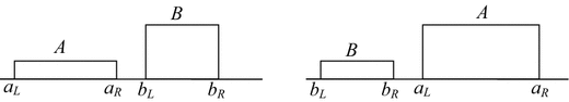

Type-1 intervals

Case 2:

These two intervals are partially related or overlapping (see Fig. 3).

Fig. 3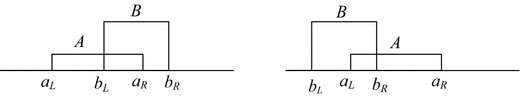

Type-2 intervals

Case 3:

Any one of the intervals contains other (see Fig. 4).

Fig. 4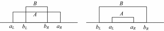

Type-3 intervals

Sahoo et al. [65] have proposed the definitions of interval order relations between two interval numbers in order to solve the maximization and minimization problems.

Definition 3

Order relation of type $>_{\hbox{max} }$ between two intervals. Let us consider two intervals $A = [a_{\text{L}} ,a_{\text{R}} ] = \left\langle {a_{\text{c}} ,a_{\text{w}} } \right\rangle$ and $B = [b_{\text{L}} ,b_{\text{R}} ] = \left\langle {b_{\text{c}} ,b_{\text{w}} } \right\rangle$. Therefore, for solving the maximization problems, the following properties hold:

• 1. $A >_{\hbox{max} } B \Leftrightarrow a_{\text{c}} > b_{\text{c}} \;{\text{for}}\;{\text{Type}}\;{\text{I}}\;{\text{and}}\;{\text{Type}}\;{\text{II}}\;{\text{intervals}},$

• 2. $A >_{\hbox{max} } B \Leftrightarrow$ either $a_{\text{c}} \ge b_{\text{c}} \wedge a_{\text{w}} < b_{\text{w}}$ or $a_{\text{c}} \ge b_{\text{c}} \wedge a_{\text{R}} > b_{\text{R}} \;{\text{for}}\;{\text{Type}}\;{\text{III}}\;{\text{intervals}},$

According to the above definition, the interval number $A$ is accepted for maximization case. So, the order relation $A >_{\hbox{max}} B$ is not symmetric, but it is reflexive and transitive.

Definition 4

Order relation of type $<_{\hbox{min} }$ between two intervals. Let us consider two interval numbers $A = [a_{\text{L}} ,a_{\text{R}} ] = \left\langle {a_{\text{c}} ,a_{\text{w}} } \right\rangle$ and $B = [b_{\text{L}} ,b_{\text{R}} ] = \left\langle {b_{\text{c}} ,b_{\text{w}} } \right\rangle$. Then, for solving the minimization problems, the following properties hold:

• 1. $A <_{\hbox{min} } \; B \Leftrightarrow a_{\text{c}} < b_{\text{c}} \;{\text{for}}\;{\text{Type}}\;{\text{I}}\;{\text{and}}\;{\text{Type}}\;{\text{II}}\;{\text{intervals}},$

• 2. $A <_{\hbox{min} } \; B \Leftrightarrow$ either $a_{\text{c}} \le b_{\text{c}} \wedge a_{\text{w}} < b_{\text{w}}$ or $a_{\text{c}} \le b_{\text{c}} \wedge a_{\text{L}} < b_{\text{L}} \;{\text{for}}\;{\text{Type}}\;{\text{III}}\;{\text{intervals}},$

According to the above definition, the interval $A$ is accepted for minimization case. So, the order relation $A \,{<_{\hbox{min} }}\, B$ is reflexive and transitive, but it is not symmetric.

$A \,{<_{\hbox{min} }}\, B$ is reflexive and transitive, but it is not symmetric.

References

Harris, F.W.: How many parts to make at once, factory. Mag. Manag. 10(2), 135–136 and 152 (1913)
Ghare, P.M., Schrader, G.F.: A model for exponentially decaying inventory. J. Ind. Eng. 14(5), 238–243 (1963)
Chen, S.C., Cárdenas-Barrón, L.E., Teng, J.T.: Retailer’s economic order quantity when the supplier offers conditionally permissible delay in payments link to order quantity. Int. J. Prod. Econ. 155, 284–291 (2014)
Haley, C.W., Higgins, R.C.: Inventory policy and trade credit financing. Manag. Sci. 20(4-part-i), 464–471 (1973)
Goyal, S.K.: Economic order quantity under conditions of permissible delay in payments. J. Oper. Res. Soc. 36(4), 335–338 (1985)
Aggarwal, S.P., Jaggi, C.K.: Ordering policies of deteriorating items under permissible delay in payments. J. Oper. Res. Soc. 46(5), 658–662 (1995)
Jamal, A.M.M., Sarker, B.R., Wang, S.: An ordering policy for deteriorating items with allowable shortages and permissible delay in payment. J. Oper. Res. Soc. 48(8), 826–833 (1997)
Emmons, H.: A replenishment model for radioactive nuclide generators. Manag. Sci. 14(5), 263–274 (1968)
Covert, R.P., Philip, G.C.: An EOQ model for items with Weibull distribution deterioration. AIIE Trans. 5(4), 323–326 (1973)
Giri, B.C., Jalan, A.K., Chaudhuri, K.S.: Economic order quantity model with Weibull deterioration distribution, shortage and ramp-type demand. Int. J. Syst. Sci. 34(4), 237–243 (2003)
Ghosh, S.K., Chaudhuri, K.S.: An order-level inventory model for a deteriorating item with Weibull distribution deterioration, time-quadratic demand and shortages. Adv. Model. Optim. 6(1), 21–35 (2004)
Chakrabarty, T., Giri, B.C., Chaudhuri, K.S.: An EOQ model for items with Weibull distribution deterioration, shortages and trended demand: an extension of Philip’s model. Comput. Oper. Res. 25(7), 649–657 (1998)
Giri, B.C., Chakraborty, T., Chaudhuri, K.S.: Retailer’s optimal policy for perishable product with shortages when supplier offers all-unit quantity and freight cost discounts. Proc. Natl. Acad. Sci. 69(A), 315–326 (1999)
Sana, S., Goyal, S.K., Chaudhuri, K.S.: A production–inventory model for a deteriorating item with trended demand and shortages. Eur. J. Oper. Res. 157(2), 357–371 (2004)
Sana, S., Chaudhuri, K.S.: On a volume flexible production policy for deteriorating item with stock-dependent demand rate. Nonlinear Phenom. Complex Syst. 7(1), 61–68 (2004)
Misra, R.B.: Optimum production lot-size model for a system with deteriorating inventory. Int. J. Prod. Res. 13(5), 495–505 (1975)
Deb, M., Chaudhuri, K.S.: An EOQ model for items with finite rate of production and variable rate of deterioration. Opsearch 23, 175–181 (1986)
Giri, B.C., Pal, S., Goswami, A., Chaudhuri, K.S.: An inventory model for deteriorating items with stock-dependent demand rate. Eur. J. Oper. Res. 95(3), 604–610 (1996)
Goswami, A., Chaudhuri, K.S.: An EOQ model for deteriorating items with shortage and a linear trend in demand. J. Oper. Res. Soc. 42(12), 1105–1110 (1991)
Bhunia, A.K., Maiti, M.: Deterministic inventory model for deteriorating items with finite rate of replenishment dependent on inventory level. Comput. Oper. Res. 25(11), 997–1006 (1998)
Bhunia, A.K., Maiti, M.: An inventory model of deteriorating items with lot-size dependent replenishment cost and a linear trend in demand. Appl. Math. Model. 23(4), 301–308 (1999)
Mandal, B.N., Phaujdar, S.: An inventory model for deteriorating items and stock-dependent consumption rate. J. Oper. Res. Soc. 40(5), 483–488 (1989)
Padmanabhan, G., Vrat, P.: EOQ models for perishable items under stock-dependent selling rate. Eur. J. Oper. Res. 86(2), 281–292 (1995)
Pal, S., Goswami, A., Chaudhuri, K.S.: A deterministic inventory model for deteriorating items with stock-dependent demand rate. Int. J. Prod. Econ. 32(3), 291–299 (1993)
Mandal, M., Maiti, M.: Inventory model for damageable items with stock-dependent demand and shortages. Opsearch 34(3), 156–166 (1997)
Goyal, S.K., Gunasekaran, A.: An integrated production-inventory-marketing model for deteriorating items. Comput. Ind. Eng. 28(4), 755–762 (1995)
Sarker, B.R., Mukherjee, S., Balan, C.V.: An order-level lot-size inventory model with inventory-level dependent demand and deterioration. Int. J. Prod. Econ. 48(3), 227–236 (1997)
Pal, A.K., Bhunia, A.K., Mukherjee, R.N.: Optimal lot size model for deteriorating items with demand rate dependent on displayed stock level (DSL) and partial backordering. Eur. J. Oper. Res. 175(2), 977–991 (2006)
Raafat, F.: Survey of literature on continuously deteriorating inventory models. J. Oper. Res. Soc. 42(1), 27–37 (1991)
Goyal, S.K., Giri, B.C.: Recent trends in modeling of deteriorating inventory. Eur. J. Oper. Res. 134(1), 1–16 (2001)
Bakker, M., Riezebos, J., Teunter, R.H.: Review of inventory systems with deterioration since 2001. Eur. J. Oper. Res. 221(2), 275–284 (2012)
Janssen, L., Claus, T., Sauer, J.: Literature review of deteriorating inventory models by key topics from 2012 to 2015. Int. J. Prod. Econ. 182, 86–112 (2016)
Summers, B., Wilson, N.: An empirical investigation of trade credit demand. Int. J. Econ. Bus. 9(2), 257–270 (2002)
Seifert, D., Seifert, R.W., Protopappa-Sieke, M.: A review of trade credit literature: opportunities for research in operations. Eur. J. Oper. Res. 231(2), 245–256 (2013)
Teng, J.T.: On the economic order quantity under conditions of permissible delay in payments. J. Oper. Res. Soc. 53(8), 915–918 (2002)
Das, B.C., Das, B., Mondal, S.K.: An integrated production inventory model under interactive fuzzy credit period for deteriorating item with several markets. Appl. Soft Comput. 28, 453–465 (2015)
Das, B.C., Das, B., Mondal, S.K.: An integrated production-inventory model with defective item dependent stochastic credit period. Comput. Ind. Eng. 110, 255–263 (2017)
Guchhait, P., Maiti, M.K., Maiti, M.: A production inventory model with fuzzy production and demand using fuzzy differential equation: an interval compared genetic algorithm approach. Eng. Appl. Artif. Intell. 26(2), 766–778 (2013)
Guchhait, P., Maiti, M.K., Maiti, M.: Inventory model of a deteriorating item with price and credit linked fuzzy demand: a fuzzy differential equation approach. Opsearch 51(3), 321–353 (2014)
Chang, C.T., Ouyang, L.Y., Teng, J.T.: An EOQ model for deteriorating items under supplier credits linked to ordering quantity. Appl. Math. Model. 27(12), 983–996 (2003)
Abad, P.L., Jaggi, C.K.: A joint approach for setting unit price and the length of the credit period for a seller when end demand is price sensitive. Int. J. Prod. Econ. 83(2), 115–122 (2003)
Ouyang, L.Y., Wu, K.S., Yang, C.T.: A study on an inventory model for non-instantaneous deteriorating items with permissible delay in payments. Comput. Ind. Eng. 51(4), 637–651 (2006)
Huang, Y.F.: An inventory model under two levels of trade credit and limited storage space derived without derivatives. Appl. Math. Model. 30(5), 418–436 (2006)
Huang, Y.F.: Economic order quantity under conditionally permissible delay in payments. Eur. J. Oper. Res. 176(2), 911–924 (2007)
Huang, Y.F.: Optimal retailer’s replenishment decisions in the EPQ model under two levels of trade credit policy. Eur. J. Oper. Res. 176(3), 1577–1591 (2007)
Sana, S.S., Chaudhuri, K.S.: A deterministic EOQ model with delays in payments and price-discount offers. Eur. J. Oper. Res. 184(2), 509–533 (2008)
Huang, Y.F., Hsu, K.H.: An EOQ model under retailer partial trade credit policy in supply chain. Int. J. Prod. Econ. 112(2), 655–664 (2008)
Ho, C.H., Ouyang, L.Y., Su, C.H.: Optimal pricing, shipment and payment policy for an integrated supplier–buyer inventory model with two-part trade credit. Eur. J. Oper. Res. 187(2), 496–510 (2008)
Bhunia, A.K., Shaikh, A.A., Sahoo, L.: A two-warehouse inventory model for deteriorating items under permissible delay in payment via particle swarm optimization. Int. J. Logist. Syst. Manag. 24(1), 45–68 (2016)
Jaggi, C.K., Tiwari, S., Shafi, A.: Effect of deterioration on two-warehouse inventory model with imperfect quality. Comput. Ind. Eng. 88, 378–385 (2015)
Jaggi, C., Sharma, A., Tiwari, S.: Credit financing in economic ordering policies for non-instantaneous deteriorating items with price dependent demand under permissible delay in payments: a new approach. Int. J. Ind. Eng. Comput. 6(4), 481–502 (2015)
Jaggi, C.K., Tiwari, S., Goel, S.K.: Credit financing in economic ordering policies for non-instantaneous deteriorating items with price dependent demand and two storage facilities. Ann. Oper. Res. 248(1–2), 253–280 (2017)
Tiwari, S., Cárdenas-Barrón, L.E., Khanna, A., Jaggi, C.K.: Impact of trade credit and inflation on retailer’s ordering policies for non-instantaneous deteriorating items in a two-warehouse environment. Int. J. Prod. Econ. 176, 154–169 (2016)
Jaggi, C.K., Yadavalli, V.S.S., Sharma, A., Tiwari, S.: A fuzzy EOQ model with allowable shortage under different trade credit terms. Appl. Math. Inf. Sci. 10(2), 785–805 (2016)
Jaggi, C., Tiwari, S., Goel, S.: Replenishment policy for non-instantaneous deteriorating items in a two storage facilities under inflationary conditions. Int. J. Ind. Eng. Comput. 7(3), 489–506 (2016)
Bhunia, A.K., Mahato, S.K., Shaikh, A.A., Jaggi, C.K.: A deteriorating inventory model with displayed stock-level-dependent demand and partially backlogged shortages with all unit discount facilities via particle swarm optimisation. Int. J. Syst. Sci. Oper. Logist. 1(3), 164–180 (2014)
Bhunia, A.K., Shaikh, A.A.: Investigation of two-warehouse inventory problems in interval environment under inflation via particle swarm optimization. Math. Comput. Model. Dyn. Syst. 22(2), 160–179 (2016)
Grzegorzewski, P.: Nearest interval approximation of a fuzzy number. Fuzzy Sets Syst. 130(3), 321–330 (2002)
Bhunia, A.K., Shaikh, A.A.: An application of PSO in a two-warehouse inventory model for deteriorating item under permissible delay in payment with different inventory policies. Appl. Math. Comput. 256, 831–850 (2015)
Kennedy, J.F., Eberhart, R.C.: Particle swarm optimization. In: Proceedings of the IEEE International Conference on Neural Network, vol. IV, Perth, Australia, pp. 1942–1948 (1995)
Clerc, M., Kennedy, J.: The particle swarm-explosion, stability, and convergence in a multidimensional complex space. IEEE Trans. Evol. Comput. 6(1), 58–73 (2002)
Clerc, M.: The swarm and the queen: towards a deterministic and adaptive particle swarm optimization: In: Proceedings of the 1999 Congress on Evolutionary Computation, 1999, CEC 99, vol. 3, pp. 1951–1957. IEEE (1999)
Sun, J., Feng, B., Xu, W.: Particle swarm optimization with particles having quantum behaviour. In: Congress on Evolutionary Computation, 2004, CEC2004, vol. 1, pp. 325–331. IEEE (2004)
Sun, J., Xu, W., Feng, B.: A global search strategy of quantum-behaved particle swarm optimization. In: 2004 IEEE Conference on Cybernetics and Intelligent Systems, vol. 1, pp. 111–116. IEEE (2004)
Sahoo, L., Bhunia, A.K., Kapur, P.K.: Genetic algorithm based multi-objective reliability optimization in interval environment. Comput. Ind. Eng. 62(1), 152–160 (2012)
Acknowledgements
We thank the editor and anonymous reviewers for their constructive feedback on earlier drafts of this manuscript. The Tecnológico de Monterrey Research Group in Industrial Engineering and Numerical Methods 0822B01006 supported the first and third authors.
Author information
Authors and Affiliations
Corresponding author