
Abstract
Data are getting larger, and most of them are necessary for our businesses. Rapid explosion of data brings us a number of challenges relating to its complexity and how the most important knowledge can be captured in reasonable time. Fuzzy C-means (FCM)—one of the most efficient clustering algorithms which have been widely used in pattern recognition, data compression, image segmentation, computer vision and many other fields—also faces the problem of processing large datasets. In this paper, we propose some novel hybrid clustering algorithms based on incremental clustering and initial selection to tune up FCM for the Big Data problem. The first algorithm determines meshes of rectangle covering data points as the representatives, while the second one considers data points that have high influence to others as the representatives. The representatives are then clustered by FCM, and the new centers are selected as initial ones for clustering of the dataset. Theoretical analyses of the new algorithms including comparison of quality of solutions when clustering the representatives set versus the entire set are examined. The experimental results on both simulated and real datasets show that total computational time of the new methods including time of finding representatives and clustering is faster than those of other relevant algorithms. The validation on clustering quality is also examined. The findings of this paper have great impact and significance to researches in the fields of soft computing and Big Data processing. It is obvious that computing methodologies nowadays are facing with huge amount of diverse and complex data structures. Speed of processing is the main priority when considering effectiveness of a specific method. The findings demonstrated practical algorithms and investigated their characteristics that could be referenced by other researchers in similar applications. The usefulness and significance of this research are clearly demonstrated within the extent of real-life applications.
1 Introduction
Fuzzy C-means (FCM) [4] is considered as a strong aid of rule extraction and data mining from a set of data in which fuzzy factors are common [7, 13]. It has been used for pattern recognition, data compression, image segmentation, computer vision and many other fields [21, 23, 29–39, 41, 43, 44, 46, 51]. Given a dataset of N attributes: X = {x 1, …, x N }, with x k ∊ R p and V = (v 1, …, v C ) being the centers of all groups. The FCM algorithm aims to minimize:
where u kj is the membership value showing the degree to which element x k belongs to cluster c j and m is the fuzzifier which determines the level of cluster fuzziness. The constraints for the optimization problem are:
Problem (1–2) is solved by an iterative schema that computes the cluster centers and the membership matrix until the difference between two consecutive iteration is smaller than a given threshold. This algorithm was proved to converge to the saddle points by Bezdek et al. [4].
Nevertheless, data tend to be huge and diverse as they can come from everywhere: sensors used to gather climate information, posts to social media sites, digital pictures and videos, purchase transaction records, and cell phone GPS signals to name a few. Some of them are even in different organizations and structures. Rapid explosion of data brings a number of challenges regarding how the most important knowledge can be captured in reasonable time. Jain [17] stated that clustering is the key to the Big Data problem since it provides efficient browsing, search, recommendation and organization of data without prior knowledge of the number and nature of groups in data. However, the FCM algorithm still faces the problem of processing large datasets. A simple and straightforward method to accelerate FCM for the Big Data problem is hence required.
Scanning the literature, we recognize that there are numbers of solutions dealing with this matter [2, 3, 10, 25, 28] including data reduction [6, 14, 15, 18, 22, 27, 49, 50], initial selection [12, 16, 24, 26, 42], suppression [5, 11, 40] and incremental clustering [1, 9, 47, 48]. Motivated by developing a simple and straightforward method to accelerate FCM for the Big Data problem, the idea of hybrid algorithms between incremental clustering and initial selection is utilized. Incremental clustering and initial selection do not require complex preprocessing procedures like other groups. Incremental clustering works based on the assumption that small representatives of the dataset could represent for the whole dataset; therefore, clustering in the representative sets obtains both fast computational speed and reasonable quality in comparison with the clustering in the entire dataset. Initial selection seeks out appropriate initial centers and makes the clustering process faster due to the closeness of the final centers with the initial ones. However, an important question regarding these approaches is how to determine such the representatives and initial centers accordingly.
In this paper, we aim to develop some novel hybrid algorithms based on incremental clustering and initial selection to tune up FCM for the Big Data problem. Specifically, the first algorithm, named as GB-FCM, determines meshes of a rectangle covering data points as the representatives whose active ones that cover at least a data point are classified into groups by the FCM algorithm. The new centers, which reflect more accurately the nature of dataset, are selected as initial centers of FCM to classify the entire dataset. The second algorithm, named as DB-FCM, considers data points that have high influence to others as the representatives. The term ‘influence’ is equivalent to the number of neighbors in a sphere whose center is a given data point. High-influence data points can be the best reduction of entire dataset. Again, these representatives are clustered by the FCM algorithm and the new centers are selected as initial ones for clustering of the dataset.
The main difference of these algorithms with the relevant ones (e.g. the standalone incremental clustering and initial selection) is how to determine the representatives and initial centers. Unlike incremental clustering that considers centers/medoids, the new algorithms choose either rectangular meshes or data points as representatives on the basis of distribution of data points. Unlike initial selection that often finds out initial centers by meta-heuristic optimization methods, the new algorithms utilize the representatives to clarify centers. These modifications do make the proposed algorithm faster and more precise than existing clustering techniques. Lastly, theoretical analyses of the new algorithms are also examined.
Rest of this paper is organized as follows. Sections 2 and 3 describe two novel methods. Section 4 experimentally validates these algorithms in comparison with the relevant ones on both simulated and real datasets. Finally, Section 5 draws the conclusions and delineates future works.
2 Grid-Based Approximation for Fuzzy Clustering
2.1 The Algorithm
The objective function and constraints of the new algorithm, named as Grid-Based Approximation for Fuzzy Clustering algorithm (GB-FCM), are expressed as follows.
where o h is the representative of the set {x k }, w h is the number of data points that o h represents and l is the number of cells.
The GB-FCM algorithm is demonstrated in Table 1. Note that in Step 2 of this algorithm, if an interval in a given axis has no or a data point inside, recursively merge it with its right interval until the number of data points is larger than or equal to 2. By this modification, each interval is assumed to contain at least 2 data points, which are dense enough for clustering.
Example 1
Consider the following dataset with the bound of data points being set up as in Step 1 of the algorithm. Herein, ɛ X = 0.5 and ɛ Y = 1 (Fig. 1).

Small dataset
According to the Step 3, we consider all meshes of the newly created rectangle as potential representatives (Fig. 2).

Possible meshes for the dataset
Rectify all meshes in Fig. 2 by Step 4, we get the active representatives in red color (Fig. 3).

Active meshes for the dataset
Use FCM to classify the active representatives in Fig. 3 into 2 groups and obtain the cluster centers represented by the triangular symbol in Fig. 4.

Use FCM for the representatives
Herein, we recognize that the achieved cluster centers are ‘nearly’ approximate to the optimal cluster centers of the original dataset. The final cluster centers are obtained by the same process of FCM with the initial solutions being extracted above (See Step 6, Fig. 5). In fact, when the number of data points is large, this method is quite efficient to quickly determine the optimal centers and results.

Final cluster centers
2.2 Theoretical Analyses of GB-FCM
Firstly, we prove that the problem in (1, 2) is equivalent to the problem in (3, 4).
Theorem 1
After replacing {x k } by its representative o h , the problem (1, 2) is reduced to minimize the alternative objective function (3) with the partition matrix U satisfying the condition ( 4 ).
Proof
From (1), we have
Apply Jensen’s inequality, we get
Therefore, from (8) and (9) we have
Because of the property of u kj , it is obvious that,
□
Theorem 2
The optimal solutions of the system (3) and (4) are
Proof
Similar to the proof of Bezdek et al. [4], we use the gradient method for the objective function \(\tilde{J}\) in (3),
Use the Lagrange multiplier, we get
Because of constraint (4), we obtain
From Eqs. (19) and (20), we have
From Eqs. (17, 21), we have the solutions of the system (3) and (4).
Theorem 2 allows us to determine the centers and the partition matrix described in Step 5 of the GB-FCM algorithm.
Theorem 3
The minimal cost of clustering representatives differs from the minimal cost of clustering the original dataset a quantity of ɛ × l.
Proof
Denote by \((\overline{{u_{kj} }} ,\overline{{v_{j} }} )\) the optimal solutions of original problem and \((\overline{\overline{{u_{hj} }}} ,\overline{\overline{{v_{j} }}} )\) the optimal solutions of representative clustering. From the minimal property of these solutions, we have
where ɛ h in (24) is the farthest distance in each set {x k } to its representative o h .
From the inequality (25), we recognize that the centers of the problem (1–2) are not too far from those of representative clustering in Eqs. (3–4).□
Next, we assess the quality of choosing representatives in GB-FCM. Let us state some definitions below.
Definition 1
The quality of a representative method is defined by a minimal number a method satisfying condition,
where s min is the optimal number of spheres with radii ɛ, s method is the number of spheres.
Definition 2
Method 1 is said to be better than method 2 if
If we consider all meshes in a grid as potential representatives, then a possible determination of a data point to any mesh is specified as follows. If for any x k in the dataset, there exists a coordinate,
then we assign x k to representatives having coordinates o j h < x j k .
Theorem 4
The quality of the grid-based method is: a gridmethod = 3 d , for which d is the number of dimensions of feature space. In the other words,
Proof
-
If d = 1: Assume that o h , o h+1, o h+2, o h+3 are the consecutive meshes (Fig. 6). For any data point having the coordinate in this dimension is y, there are three possible cases.
Fig. 6 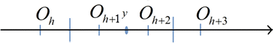
Determine a suitable mesh for representing data points having coordinate y
-
Case 1: If y < (o k+1 + o k+2)/2, all data points that y represents would be represented by o h , o h+1, o h+2.
-
Case 2: If y > (o k+1 + o k+2)/2, all data points that y represents would be represented by o h+1, o h+2, o h+3.
-
Case 3: Ify = (o k+1 + o k+2)/2, all data points that |y - x k | < ɛ would be represented by o h , o h+1, o h+2. The left endpoint certainly belongs to o h . The right endpoint is assigned to o h+2 because it is less than (o h+2 + o h+3)/2.
In this dimension, we need three representatives for an optimal representative y.
-
-
If d > 1: It is due to the fact that in every dimension, we need the maximum three rows of representatives. Thus, in d dimensions, we totally need 3d representatives (Fig. 7)□
Fig. 7 
Determine number of representatives when the dimension is greater than 1


Example 2
In Fig. 8, the point x 1 is assigned to o h+3, x 2 is assigned to o h .

Example of mesh determination and representatives for {x 1, x 2}
3 Density-Based Approximation for Fuzzy Clustering
3.1 The Algorithm
In this section, we introduce another algorithm, named as Density-Based Approximation for Fuzzy Clustering Method (DB-FCM). The descriptions of this algorithm are shown in Table 2. Note that in Step 5, new representative of merged sphere is calculated by the average value of old representatives. In cases that there is only one sphere for the whole dataset after merging, return to Step 1 with a different initial data point. If the results of two consecutive initializations are identical, stop the algorithm.
Example 3
Consider the dataset in Example 1 (Fig. 1). Herein, ɛ X = 0.5 and ɛ Y = 1 so ɛ = 1.118. Steps 1–4 create some representatives of the sphere with radius ɛ (Fig. 9). The red points are the centers of the spheres.

Forming spheres
Use FCM to classify the centers into 2 groups, and finally perform FCM again to classify the original dataset with the initial centers of the previous steps, we get the results in Fig. 10. Notice that these steps are analogous to those in GB-FCM.

Final cluster centers of DB-FCM
3.2 Theoretical Analyses of DB-FCM
Firstly, from Definition 1, we would like to know whether or not the quality of DB-FCM is better than that of GB-FCM. The following theorem helps us answer this question.
Theorem 5
DB-FCM is better than GB-FCM. In other words,
Proof
We recognize that a densitybased is the maximal number of spheres whose centers lie in a given radius sphere and their distances are greater than ɛ. It comes from the fact that data points belong to one sphere representative only, and the next representative must not belong to any previous sphere representative (Fig. 11). By the condition centers in the given sphere, the problem can be changed to finding the maximal number of spheres with radii ɛ/2 that can be put into a sphere with radius 3ɛ/2 (Fig. 12). Besides, all spheres with radii ɛ/2 are not allowed to touch together. Obviously, this property is equivalent to the fact that distances of centers are greater than ɛ. When all centers are in the boundary of the given sphere of the original problem, the spheres with radii ɛ/2 touch the boundary of the sphere with radius 3ɛ/2.

Data points belong to the red sphere representative only

Alternative problem: finding maximal number of spheres in a red sphere
a densitybased is the maximal number of spheres with radii ɛ/2 that can be put into a sphere with radius 3ɛ/2. It is less than or equal to the maximal number of spheres if we dismiss the condition that spheres do not touch together. We know the volume,
where A d is a constant in d dimensional space. Because spheres with radii ɛ/2 lie in the sphere with radius 3ɛ/2, the maximal number of spheres is less than or equal to,
However, this number cannot be 3d because in that situation, data points in the sphere with radius 3ɛ/2 are covered by spheres with radius ɛ/2. In fact, the number of intersections between spheres with radii ɛ/2 and the sphere with radius 3ɛ/2 is limited. Indeed, a limited number of points in the boundary of the sphere with radius 3ɛ/2 are covered by spheres with radii ɛ/2. Therefore, the quality of density-based method is better than the one of the grid-based and satisfies the inequality,
Theorem 6
(A better representative method in the dimension that is smaller than three—half-sphere representative method).
In fact, the half-sphere representative method is also iterative. Initially, we fix a dimension, then iterate.
-
Choose the point having the smallest value on that dimension. Scan all points that lie in the half-sphere with radius 2ɛ.
-
Replace the half-sphere by a set of spheres whose radii cover all its points.
At the first iteration, the half-sphere representative is the pole in a fixed dimension (Fig. 13). In next steps of iteration, the representative is the lowest point in the remaining part of some optimal representative sphere (Fig. 14).

Representative is the red point which has smallest value among all

Representative is the lowest point in the remaining part of representative sphere
In one-dimensional space, it is just the interval width of ɛ. The a halfsphere in this case is equal to one. This means that the number of representatives chosen by the half-sphere method is minimal. In addition, it is easy to check that a densitybased = 2. In two-dimensional space, a densitybased ≥ 5, because we can arrange five spheres with radii ɛ/2 in a sphere with radius 3ɛ/2 (Fig. 15). Thus, we just need four spheres with radii ɛ to cover a sphere with radius 2.ɛ. The set of four spheres are constructed by putting a sphere with the center is the midpoint of the cut line of the half-sphere, then drawing a half of hexagon and putting three left spheres’ centers in the midpoints of edges of this half hexagon. Thus, in two-dimensional space, a halfsphere ≤ 4. It follows that the half-sphere representative method in this case is better than the density-based method. In fact, a halfsphere is the minimal number of spheres with radii ɛ to cover a sphere with radius 2.ɛ.

Five spheres with radii ɛ/2 can be arranged in a sphere with radius 3ɛ/2
4 Results
4.1 Experimental Environment
-
Experimental tools: We have implemented the proposed algorithms (GB-FCM and DB-FCM) in addition to FCM [4] and the stand-alone methods of initial selection—psFCM [16], suppression—neural network [5] and incremental clustering—FHCA [9] in C programming language and executed them on a Linux Cluster 1350 with eight computing nodes of 51.2GFlops. Each node contains two Intel Xeon dual core 3.2 GHz, 2 GB Ram.
-
Experimental datasets: We use six simulated (D 1–D 6) and four real (T 1–T 4) datasets described in Table 3.
Table 3 Descriptions of the datasets -
Simulated datasets: Datasets from D 1 to D 3 are generated from a Gaussian distribution by using the Marsaglia [20] method. The standard deviation of these data points in each cluster is one. The dimension of these datasets is two. The datasets from D 4 to D 6 are also generated from a Gaussian distribution, but in the five-dimensional space;
-
Real datasets: they are taken from UCI KDD Archive Website [45]. T 1 is Forest CoverType including 581012 instances in 54 dimensions showing the actual forest cover type for a given observation (30 × 30 m cell) determined from US Forest Service (USFS) Region 2 Resource Information System (RIS). T 2 is a text dataset namely Enron Emails in Bag of Words Data Set including 39,861 numbers of documents, 28,102 numbers of words in the vocabulary and 3,710,420 number of words in total. T 3 is a multivariate and text dataset, namely KEGG Metabolic Relation Network (Directed) including 53,414 instances in 24 dimensions. T 4 namely NYSK (New York v. Strauss-Kahn) is a collection of English news articles about the case relating to allegations of sexual assault against the former IMF director Dominique Strauss-Kahn (May 2011) including 10,421 instances in 7 dimensions.
-
-
Cluster validity measurement: Davies-Bouldin (DB) index [8] in Eqs. (38–40) to evaluate the clustering qualities. In these equations, T i is the size of cluster ith, S i is a measure of scatter within the cluster and M ij is a measure of separation between cluster ith and jth. The minimum value indicates the better performance for DB index.
$$DB = \frac{1}{C}\sum\limits_{i = 1}^{C} {\left( {\mathop {\hbox{max} }\limits_{j:j \ne i} \left\{ {\frac{{S_{i} + S_{j} }}{{M_{ij} }}} \right\}} \right)}$$(38)$$S_{i} = \sqrt {\frac{1}{{T_{i} }}\sum\limits_{j = 1}^{{T_{i} }} {\left| {X_{j} - V_{i} } \right|^{2} } } ,\quad (i = \overline{1,C} )$$(39)$$M_{ij} = \left\| {V_{i} - V_{j} } \right\|,\;(i = \overline{1,C} ,\;j = \overline{1,C} ,\;i \ne j),$$(40) -
Objective:
-
To compare the total computational time of algorithms;
-
To compare the computational time of algorithms for finding representatives;
-
To measure the clustering qualities of algorithms.
-
4.2 The Comparison of the Total Computational Time
In this section, we compare the total computational time of all algorithms illustrated in Table 4. It is obvious that the computational time of the proposed methods (GB-FCM and DB-FCM) is smaller than those of other algorithms. Thus, the first remark from the experiments is that the proposed algorithms are faster than the relevant ones.
In what follows, we measure the computational time of all algorithms per data point. The results in Table 5 show that GB-FCM is the most effective algorithm because it takes smallest computational time to process a data point. The average results also demonstrate that FHCA is the worst algorithm for this matter.
Analogously, the comparison of computational time of all algorithms per the number of clusters in Table 6 also shows that GB-FCM is the most effective algorithms. This is the second remark from the experiments.
Next, we find out which algorithm is the most effective in all types of data (simulated and real). The results from Tables 4, 5 and 6 clearly show that GB-FCM is the fastest algorithm among all. Just to give an example: the computational time of GB-FCM on D 4 is 4.31, 11.49, 7.1, 10.8 and 140 times faster than those of DB-FCM, FCM, psFCM, neural network and FHCA, respectively. This is the third remark from the experiments.
4.3 The Comparison of the Computational Time for Finding Representatives
In Table 7, we describe the number of representatives and the related computational time of algorithms. The results show that GB-FCM finds representatives faster than DB-FCM and other algorithms. However, the number of representatives produced by GB-FCM is larger than that by DB-FCM.
Now, we illustrate the dataset D 1 (Fig. 16), the representatives and their centers produced by GB-FCM (Fig. 17) and DB-FCM (Fig. 18).

Dataset D 1

Clustering results of GB-FCM with centers marked in red

Clustering results of DB-FCM with centers marked in red
4.4 The Comparison of Clustering Quality
Table 8 measures the DB values of algorithms. The results reveal that the DB values of the proposed algorithms are approximate to that of FCM and mostly smaller than those of the relevant works. Moreover, the statement in Theorem 5 affirming that the clustering quality of DB-FCM is better than that of GB-FCM has been verified.
4.5 Summary of the Findings
It has been observed from the experimental results in Sections 4.2–4.4 that clustering qualities of the proposed works (GB-FCM and DB-FCM) are approximate to that of FCM and mostly better than those of other algorithms. It is understandable because FCM is the original clustering algorithm while others are the approximate methods, which were created to handle the problem of processing large datasets. According to Fig. 19 where the average DB values of all algorithms are illustrated, we realize that the clustering quality of DB-FCM is better than psFCM, neural network and FHCA. GB-FCM is approximate to these algorithms in terms of clustering quality. The clustering quality of DB-FCM is better than those of other algorithms because it creates good representations through the process of forming and merging ‘weak’ clusters into ‘strong’ ones. Therefore, cluster centers are nearly identical to the optimal results. In GB-FCM, the representatives are fixed into meshes of the grid, which somehow do not reflect the nature of dataset, thus making the limitation of GB-FCM regarding clustering quality as compared with DB-FCM. Thus, when selecting an approximation algorithm that has good clustering quality, DB-FCM is the first choice.

Average DB values of all algorithms
In terms of computational time (which is the main issue of approximation algorithms), GB-FCM shows the superiority versus other algorithms: It is faster than the relevant ones by various types of data. As illustrated in Fig. 20 where the average computational time of all algorithms per (a) data points and (b) clusters is described, two proposed algorithms are faster than others due to the idea of hybrid mechanism between incremental clustering and initial selection mentioned in the Introduction. That is to say, we have appropriate methods to determine the representatives and initial centers in GB-FCM and DB-FCM. Therefore, clustering in the representative sets obtains both fast computational speed and reasonable quality in comparison with the clustering in the entire dataset. Moreover, since the closeness of the final centers with the initial ones, those algorithms would converge to the final results faster than other methods. The results in Tables 5, 6 and Fig. 20 have clearly demonstrated this fact. It should be noted that when selecting an approximation algorithm that has good computing speed, GB-FCM is the first choice.

Average computational time of all algorithms per (a) data points; (b) clusters
Last but not least, the verification on the representatives showed that GB-FCM finds representatives faster than other algorithms and the number of representatives of DB-FCM is smaller than those of other algorithms. This remark should be noted when finding an algorithm that has both fast computing speed and low memory space of data storage. In some cases when the memory of storage is limited, DB-FCM is a good choice to use.
We have analyzed the reason why the proposed algorithms perform better than the others in terms of clustering quality, computation time and the representatives. Also, their advantages and disadvantages have been identified to make them feasible in practical applications.
5 Conclusions
In this paper, we proposed two novel hybrid clustering algorithms namely GB-FCM and DB-FCM based on incremental clustering and initial selection to tune up FCM for the Big Data problem. Details of the algorithms including a series of theorems were described. The theoretical contributions of the new algorithms are: i) the equivalence of clustering in the representative sets to that in the entire set; ii) difference of solutions of the representative sets vs. those of the entire set that demonstrates clustering quality of the new algorithms; iii) the definition of quality; iv) the estimation of clustering quality of the new methods; v) the half-sphere representative. We also proved that the quality of solutions when clustering the representatives set is approximate to that of clustering the original dataset. Such analyses would help explaining the algorithms better. The proposed algorithms were verified experimentally on both simulated and real datasets. The results showed that the new algorithms run faster than other relevant methods. Analyses about the clustering qualities of algorithms and representatives were performed accordingly. Further researches on this theme will extend the half-sphere representative method to the dimension greater than two. Moreover, a more exact bound for the density-based method will be considered.
References
Aaron, B., Tamir, D., Rishe, N., Kandel, A.: Dynamic incremental fuzzy C-means clustering. In: 6th International Conferences on Pervasive Patterns and Applications (PATTERNS 2014), pp. 28–37 (2014)
Anderson, D.T., Luke, R.H., Keller, J.M.: Speedup of fuzzy clustering through stream processing on graphics processing units. IEEE Trans. Fuzzy Syst. 16(4), 1101–1106 (2008)
Arora S., Chana, I.: A survey of clustering techniques for big data analysis. In: 2014 5th IEEE International Conference on the Next Generation Information Technology Summit (Confluence), pp. 59–65 (2014)
Bezdek, J.C., Ehrlich, R., Full, W.: FCM: the fuzzy c-means clustering algorithm. Comput. Geosci. 10(2), 191–203 (1984)
Borgelt, C., Kruse R.: Speeding up fuzzy clustering with neural network techniques. In: Proceeding of the 12th IEEE International Conference on Fuzzy Systems (FUZZ ‘03), St. Louis, Missouri, USA, Vol. 2, pp. 852–856 (2003)
Cheng, T.W., Goldgof, D.B., Hall, L.O.: Fast fuzzy clustering. Fuzzy Sets Syst. 93(1), 49–56 (1998)
Cuong, B.C., Son, L.H., Chau, H.T.M.: Some context fuzzy clustering methods for classification problems. In: Proceedings of the 2010 Symposium on Information and Communication Technology, Hanoi, Vietnam, pp. 34–40 (2010)
Davies, D.L., Bouldin, D.W.: A cluster separation measure. IEEE Trans. Patt Anal. Mach. Intell. 2, 224–227 (1979)
Dong, Y., Zhuang, Y.: Fuzzy Hierarchical clustering algorithm facing large databases. In: Proceeding of the 5th IEEE World Congress on Intelligent Control and Automation, Hangzhou, China, Vol. 5, pp. 4282–4286 (2004)
Fahad, A., Alshatri, N., Tari, Z., Alamri, A., Khalil, I., Zomaya, A.Y., Foufou, S., Bouras, A.: A survey of clustering algorithms for big data: taxonomy & empirical analysis. IEEE Trans. Emerg. Top. Comput. 2(3), 267–279 (2014)
Fan, J., Li, J.: A fixed suppressed rate selection method for suppressed fuzzy c-means clustering algorithm. Appl. Math. 5, 1275–1283 (2014)
Feng, X.B., Yao, F., Li, Z.G., Yang, X.J.: Improved fuzzy C-means based on the optimal number of clusters. Appl. Mech. Mater. 392, 803–807 (2013)
Gobi, A.F., Pedrycz, W.: The potential of fuzzy neural networks in the realization of approximation reasoning engines. Fuzzy Sets Syst. 157(22), 2954–2973 (2006)
Hall, L.O.: Exploring big data with scalable soft clustering. In: Synergies of Soft Computing and Statistics for Intelligent Data Analysis, pp. 11–15. Springer, Berlin (2013)
Hu, Y., Qu, F., Wen, C.: An unsupervised possibilistic c-means clustering algorithm with data reduction. In: 10th IEEE International Conference on Fuzzy Systems and Knowledge Discovery (FSKD 2013), pp. 29–33 (2013)
Hung, M. C., Yang, D.L. An efficient Fuzzy C-means clustering algorithm. In: Proceedings of the IEEE International Conference on Data Mining 2001 (ICDM 2001), San Jose, CA, USA, pp. 225–232 (2001)
Jain, A.K.: Data clustering: 50 years beyond K-means. Pattern Recogn. Lett. 31(8), 651–666 (2010)
Kothari, D., Narayanan, S.T., Devi, K.K.: Extended fuzzy C-means with random sampling techniques for clustering large data. Int. J. Innov. Res. Adv. Eng. 1(1), 1–4 (2014)
Levy, R.: Probabilistic models in the study of language, Ms. University of California, San Diego (2010)
Marsaglia, G.: Random variables and computers. In: Information Theory Statistical Decision Functions Random Process, pp. 499–510 (1962)
Ozturk, C., Hancer, E., Karaboga, D.: Improved clustering criterion for image clustering with artificial bee colony algorithm. Pattern Anal. Appl. 18(3), 587–599 (2015)
Parker, J.K., Hall, L.O.: Accelerating fuzzy-c means using an estimated subsample size. IEEE Trans. Fuzzy Syst. 22(5), 1229–1244 (2014)
Parvin, H., Minaei-Bidgoli, B.: A clustering ensemble framework based on selection of fuzzy weighted clusters in a locally adaptive clustering algorithm. Pattern Anal. Appl. 18(1), 87–112 (2015)
Qu, F., Hu, Y., Xue, Y., Yang, Y.: A modified possibilistic fuzzy c-means clustering algorithm. In: 2013 IEEE 9th International Conference on Natural Computation (ICNC 2013), pp. 858–862 (2013)
Rahimi S., Zargham M., Thakre A., Chhillar D.: A parallel Fuzzy C-Mean algorithm for image segmentation. In: Proceeding of the IEEE Annual Meeting of the Fuzzy Information Processing Society (NAFIPS ‘04), Vol. 1, pp. 234–237 (2004)
Ramathilagam, S., Devi, R., Kannan, S.R.: Extended fuzzy c-means: an analyzing data clustering problems. Cluster Comput. 16(3), 389–406 (2013)
Sarma, T.H., Viswanath, P., Reddy, B.E.: Speeding-up the kernel k-means clustering method: a prototype based hybrid approach. Pattern Recogn. Lett. 34(5), 564–573 (2013)
Shirkhorshidi, A.S., Aghabozorgi, S., Wah, T.Y., Herawan, T.: Big data clustering: a review. In: Computational Science and its Applications–ICCSA 2014 (pp. 707–720). Springer International Publishing (2014)
Son, L.H., Cuong, B.C., Lanzi, P.L., Thong, N.T.: A novel intuitionistic fuzzy clustering method for geo-demographic analysis. Expert Syst. Appl. 39(10), 9848–9859 (2012)
Son, L.H., Cuong, B.C., Long, H.V.: Spatial interaction—modification model and applications to geo-demographic analysis. Knowl. Based Syst. 49, 152–170 (2013)
Son, L.H., Lanzi, P.L., Cuong, B.C., Hung, H.A.: Data mining in GIS: A novel context-based fuzzy geographically weighted clustering algorithm. Int. J. Mach. Learn. Comput. 2(3), 235–238 (2012)
Son, L.H.: Enhancing clustering quality of geo-demographic analysis using context fuzzy clustering type-2 and particle swarm optimization. Appl. Soft Comput. 22, 566–584 (2014)
Son, L.H.: HU-FCF: a hybrid user-based fuzzy collaborative filtering method in recommender systems. Expert Syst. Appl. 41(15), 6861–6870 (2014)
Son, L.H.: Optimizing municipal solid waste collection using chaotic particle swarm optimization in GIS based environments: a case study at Danang City, Vietnam. Expert Syst. Appl. 41(18), 8062–8074 (2014)
Son, L.H.: DPFCM: A novel distributed picture fuzzy clustering method on picture fuzzy sets. Expert Syst. Appl. 42(1), 51–66 (2015)
Son, L.H.: Dealing with the new user cold-start problem in recommender systems: a comparative review. Inform. Syst. 58, 87–104 (2015)
Son, L.H.: HU-FCF++: a novel hybrid method for the new user cold-start problem in recommender systems. Eng. Appl. Artif. Intell. 41, 207–222 (2015)
Son, L.H., Linh, N.D., Long, H.V.: A lossless DEM compression for fast retrieval method using fuzzy clustering and MANFIS neural network. Eng. Appl. Artif. Intell. 29, 33–42 (2014)
Son, L.H., Thong, N.T.: Intuitionistic fuzzy recommender systems: an effective tool for medical diagnosis. Knowl.-Based Syst. 74, 133–150 (2015)
Szilágyi, L., Szilágyi, S.M.: Generalization rules for the suppressed fuzzy c-means clustering algorithm. Neurocomputing 139, 298–309 (2014)
Szilagyi, L., Denesi, G., Szilagyi, S.M.: Fast color reduction using approximative c-means clustering models. In: 2014 IEEE International Conference on Fuzzy Systems (FUZZ-IEEE 14’), pp. 194–201 (2014)
Taherdangkoo, M., Bagheri, M.H.: A powerful hybrid clustering method based on modified stem cells and Fuzzy C-means algorithms. Eng. Appl. Artif. Intell. 26(5), 1493–1502 (2013)
Thong, N.T., Son, L.H.: HIFCF: an effective hybrid model between picture fuzzy clustering and intuitionistic fuzzy recommender systems for medical diagnosis. Expert Syst. Appl. 42(7), 3682–3701 (2015)
Thong, P.H., Son, L.H.: A new approach to multi-variables fuzzy forecasting using picture fuzzy clustering and picture fuzzy rules interpolation method. In: Proceeding of 6th International Conference on Knowledge and Systems Engineering (KSE 2014), Hanoi, Vietnam, pp 679–690 (2014)
UCI Machine Learning Repository. (2015). Datasets, Available at: https://archive.ics.uci.edu/ml/datasets.html. Accessed: 11/03/2015
Wang, J., Chung, F.L., Wang, S., Deng, Z.: Double indices-induced FCM clustering and its integration with fuzzy subspace clustering. Pattern Anal. Appl. 17(3), 549–566 (2014)
Wang, Y., Chen, L., Mei, J.P.: Incremental fuzzy clustering with multiple medoids for large data. IEEE Trans. Fuzzy Syst. 22(6), 1557–1568 (2014)
Zang, X., Vista IV, F.P., Chong, K.T.: Fast global kernel fuzzy c-means clustering algorithm for consonant/vowel segmentation of speech signal. J Zhejiang Univ. Sci. C 15(7), 551–563 (2014)
Zhang, Q., Chen, Z.: A weighted kernel possibilistic c-means algorithm based on cloud computing for clustering big data. Int. J. Commun Syst 27(9), 1378–1391 (2014)
Zhang, Z., Havens, T.C.: Scalable approximation of kernel fuzzy c-means. In: 2013 IEEE International Conference on Big Data, pp. 161–168 (2013)
Zhao, Y., Wu, X., Kong, S.G., Zhang, L.: Joint segmentation and pairing of multispectral chromosome images. Pattern Anal. Appl. 16(4), 497–506 (2013)
Acknowledgments
The authors are greatly indebted to the editor-in-chief, Prof. Shun-Feng Su and anonymous reviewers for their comments and their valuable suggestions that improved the quality and clarity of paper. A great thank was dedicated to Msc. Nguyen Duc Thien for his discussion and supports in theoretical validation of this paper. We acknowledge the Center for High Performance Computing, VNU for running the codes in the IBM 1350 system.
Author information
Authors and Affiliations
Corresponding author
Rights and permissions
About this article

Cite this article
Son, L.H., Tien, N.D. Tune Up Fuzzy C-Means for Big Data: Some Novel Hybrid Clustering Algorithms Based on Initial Selection and Incremental Clustering. Int. J. Fuzzy Syst. 19, 1585–1602 (2017). https://doi.org/10.1007/s40815-016-0260-3
Received:
Revised:
Accepted:
Published:
Issue Date:
DOI: https://doi.org/10.1007/s40815-016-0260-3