A Method for Optimization of Five-Phase Induction Machines Based on Genetic Algorithms

Abstract

The optimization of five-phase induction machines is addressed using a new procedure based on genetic algorithms. A constrained optimization model is introduced which considers the main machine dimensions as free variables. Number of stator and rotor slots, winding pitch, and rotor bar inclination angle are among the free design variables. In addition, the relationship between fundamental and third harmonic component of the airgap induction is also considered as a free variable. This relationship is used to shape the airgap induction making it near to a trapezoid, thus potentially increasing the output torque. The underlying machine model used in the optimization process is detailed in previous works and includes the effect of losses and saturation on the steady state performance. Thus, a mixed-integer optimization problem is defined, in which the continuous variables are codified as integer variables making the optimization problem easier to solve. Three objective functions are defined and tested: efficiency, cost of conductor material, and a weighted combination of efficiency and material costs; other objective functions can be defined, too. The proposed method was applied to the optimization of a 5.5-kW prototype machine, and the results are presented and discussed.

1 Introduction

Induction machines have widely been used in virtually all kinds of application due their excellent characteristics in terms of robustness, low maintenance, production costs, and high overload capacity. Furthermore, squirrel cage induction machines are very well suited for operation in explosive atmosphere and other hazard areas, where other types of machines cannot be applied. When fed from a high-efficiency power converter, they become suitable for applications requiring accurate speed, torque, or position control. Thus, they are nowadays able to replace the dc machine in almost any kind of application.

In the last two decades, the interest on induction machines with high number of phases—i.e., machines with more than three phases—has increased considerably. This is due the fact that this type of machine, when fed by a static inverter, can present several relevant advantages when compared to conventional three-phase machines. The most outstanding of these advantages are: improved torque/volume relation, fault tolerance, and higher degree of active material utilization. However, some of these advantages are only obtained when the airgap induction differs from a sinusoid and assumes a more flattened waveform (almost trapezoidal waveform), which can be produced by imposing a third harmonic component to the stator current, as presented in Toliyat et al. (1991), Jacobina et al. (2004), Scharlau et al. (2008), Pereira et al. (2012).

To take advantage of the special characteristics of high-phase machines, new design concepts and new strategies for their control have been developed. However, an important issue, not yet deeply investigated, is the determination of the best combination of design parameters, along with the optimal percentage of third harmonic component in the airgap induction, which will result in an optimized machine with regard to a given objective function—conductor volume, for example. In this context, the main topic of this paper is the optimization of five-phase machines using a new method based on genetic algorithms. The proposed optimization model can not only be applied to define an optimized design, but also allows to take full advantage of the additional design alternatives of high-phase machines.

In general, induction machines have been designed based on a trial-and-error approach, seeking to meet legislation and standards requirements, as well as other application requirements, at a minimum cost. The success of this approach relies basically on the number of attempts made and also largely on the designers experience. The first improvement in this procedure took place in the early 1960s when computers were introduced into the design process. From then on, designers became able to evaluate a significantly larger number of design alternatives and parameter combinations in a shorter time. As a result, the machine performance could be much improved and the production costs reduced (Veinott 1956, 1960; Herzog et al. 1959; Godwin 1959; Andersen 1967; Chalmers and Bennington 1967).

Significant advancements in the automated induction machine design were possible with the formulation of design problems using optimization models containing the definition of an objective function. In Erlicki and Appelbaum (1965), for example, an unconstrained optimization problem is presented which allows to minimize the annual cost while accounting for material costs, iron losses, joule losses, along with mechanical losses. According to this model, a parametric optimization is performed in which each parameter is considered and adjusted individually while keeping the others constant. Furthermore, in Ramarathnam and Desai (1971), a mathematical formulation of a constrained optimization problem is presented which uses eleven independent variables and whose main objective is to minimize active material costs—cost of copper, aluminum, and iron—of three-phase induction machines. In this work, the optimization problem was solved using a technique known as sequential unconstrained minimization technique (SUMT). In addition, aiming at improving the convergence characteristics of the method used in Ramarathnam and Desai (1971), a comparison of five different minimization algorithms applied to the same problem is addressed in Ramarathnam et al. (1973). SUMT was also successfully applied together with the Rosenbrock method of nonlinear optimization in Singh et al. (1983) and Fetih and El-Shewy (1986).

A sequential approach to optimization problems was first introduced in Tindall and Calvert (1977) and comprised three stages defined as: (i) statement of the design specification and definition of an initial design, (ii) modification of the initial design in order to achieve a feasible design, and (iii) optimization of the feasible design considering predefined objectives. Although the stage (iii) is specifically dedicated to the optimization of the initial design, the results produced in this stage showed practically no differences when compared to the initial feasible design. Furthermore, by the time Tindall and Calvert (1977) was published, there were few concerns regarding the convexity of the optimization models. Due to this fact, great part of the efforts was directed to the nonlinearity of the model and how it could be mathematically treated. On the other hand, the discrete nature of some variables has raised concerns in such a way that part of the efforts was spent in handling these variables. In such a context, an approximation to the solution obtained with optimization models was proposed in Appelbaum et al. (1987) which accounted for the constructive feasibility of three-phase induction machines. The authors stated the optimization problem by classifying the design parameters into three different groups: variables, variable constants, and constants. Variable constants were used to handle parameters which described very complicated constraints or discrete variables, whose representation was considered difficult for the approach adopted by the time Appelbaum et al. (1987) was published. In addition, an auxiliary procedure was employed to update the variable constants during the optimization process. Therefore, the optimization model actually used continuous variables, and the generated solutions were externally adjusted to fit them into the allowable range of the discrete variables.

In the late 1980s, a detailed multi-criteria approach to the design of three-phase machines was presented, yet using classical optimization methods based on successive quadratic programming (Jazdzynski 1989). Later, multi-objective methods were also applied to design optimization of three-phase machines, thus making possible obtaining a set of solutions known as Pareto-optimal solutions (Liuzzi et al. 2003; Le Besnerais et al. 2008; Chun et al. 2008). Based on these solutions, the decision-maker can choose the best solution applying a criterion to quantify the relevance of each objective. When the weight of each objective is known beforehand, the solution selected by the decision-maker is the same obtained for an equivalent problem with only one objective function, which is defined as the weighted summation of the objectives, as described in Duan and Harley (2011).

A significant change in the methods for design optimization took place with the introduction of heuristic optimization methods (Moses et al. 1994; Bianchi and Bolognani 1998; Idir et al. 1998; Liuzzi et al. 2003; Le Besnerais et al. 2008; Chun et al. 2008; Duan and Harley 2011). Compared to classical methods, they have several advantages: It is possible to work with non-convex functions with multiple local minima; the discrete nature of variables can be considered in the problem formulation; it is possible to include arbitrary, nonlinear relationships between the variables. However, constructive constraints can lead to creation of new local minima in the objective function, as shown in Duan and Harley (2011) based on an example which uses the number of stator winding coils as a constraint. Given that the existence of local minima was already known to the authors in Ramarathnam and Desai (1971), Ramarathnam et al. (1973), Appelbaum et al. (1987), Moses et al. (1994), Bianchi and Bolognani (1998), two strategies were basically used to avoid local minima, which are based on: (i) the use of different initial solutions, as for example in Ramarathnam and Desai (1971), Ramarathnam et al. (1973), and (ii) the experience of the designer, as in Singh and Sarkar (1992).

Motivated by the possibility of avoiding local minima, several heuristic techniques have been successfully applied to the design of induction machines; among others, the following techniques deserve mention: Monte Carlo (Moses et al. 1994), error-based search (Idir et al. 1998), genetic algorithm (Bianchi and Bolognani 1998; Le Besnerais et al. 2008; Duan and Harley 2011), controlled random search (Liuzzi et al. 2003), and particle swarm optimization (Duan and Harley 2011).

Different from the works cited above, the present paper presents a method for the optimization of five-phase machines which accounts for the specific aspects of this type of machine such as the use of the third harmonic airgap induction to improve the machine performance. The underlying steady state model used to describe the machine behavior is described in Pereira et al. (2015), where an experimental validation under several working conditions is also presented. The optimization method proposed is based on genetic algorithms in which three different objective functions are considered: efficiency, costs, and a combination of both using weighting factors. In addition, geometrical constraints and specific loading limits are also taken into account (e.g., peak airgap induction, stator and rotor current density).

The main contributions of this paper are as follows:

• i. the main machine dimensions—such as the stator inner radius, the airgap length, the shape of the slots of stator and rotor—are described in such a way that only geometrically viable solutions are evaluated. As a consequence, the parametrization does not require any dimensional adjustments during the optimization process. This helps reduce the search space significantly, as only attractive and feasible solutions are effectively evaluated;

• ii. besides the main dimensions, the optimization model also optimizes the winding characteristics (e.g., winding pitch, number of winding turns, number of stator and rotor slots, inclination angle of the rotor bars, cross section of the rotor end-rings), along with the relationship between fundamental and third harmonic induction, used to modulate the spatial distribution of the induction in the airgap;

• iii. according to the proposed approach, it is possible to consider objective functions of different nature, including multi-objective functions as described, for instance, in Jazdzynski (1989), Moses et al. (1994), Liuzzi et al. (2003), Le Besnerais et al. (2008), Chun et al. (2008);

• iv. based on concepts of genetic algorithms, a new algorithm is developed to solve the optimization model. This algorithm uses integer codification so that all defined operators are capable of handling integer variables. Furthermore, it has an explicit diversity control of the population to prevent premature convergence. Finally, the algorithm does a local search around the best solutions (intensification).

2 Variables Used for the Machine Design

In the approach followed here, the design of the induction machine is based on a large number of variables, which will be referred as design variables; the most part of them are related to the machine dimensions and slot shapes, whereas one variable is related to the stator voltage waveform ($K_{31}$), which is used to impose the waveform of the airgap induction. The variables which define the stator dimensions are shown in Fig. 1. Further, to reduce the number of possible solutions to be evaluated during the optimization process, the stator winding is assumed to be of low-voltage type; consequently, the slot shape of the stator is assumed to be trapezoidal with rounded base (see Fig. 1). In what follows, the design variables are described.

• $b_{1s}$—stator slot width at the base;

  Fig. 1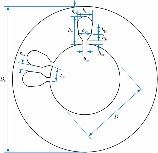

  

  Dimensions of the stator with trapezoidal shape slots and rounded base

• $b_{3s}$—stator slot width at the bottom of the region containing conductors;

• $b_{os}$—stator slot opening;

• $b_{zs}$—stator tooth width;

• D—stator inner diameter;

• $D_{e}$—stator outer diameter;

• $h_{1s}$—stator slot height in the region containing conductors;

• $h_{3s}$—height of the stator slot in the transition region;

• $h_{cs}$—stator yoke height;

• $h_{cs}^\text {min}$—minimum value of stator yoke height;

• $h_{os}$—height of the opening channel of the stator slot;

• $h_{zs}$—stator tooth height;

• m—stator phase number;

• $N_{s}$—number of stator slots;

• $N_{c}$—number of stator winding layers;

• p—number of pole pairs;

• q—number of slots per phase and pole of the stator;

• $Y_{p}$—stator winding pitch given in slots;

• $\tau _{ns}$—stator slot pitch.

The variables used for the design of the rotor cage, which has a triangular slot closure as shown in Fig. 2, are defined as follows:

• $b_{1r}$—rotor slot width at the base;

  Fig. 2

  

  Dimensions of the rotor with triangular slot closure

• $b_{3r}$—rotor slot width;

• $b_{zr}$—rotor tooth width;

• $b_{ar}$—width of the rotor end-ring;

• $D_{ex}$—shaft diameter;

• $h_{1r}$—rotor slot height in the region containing conductors;

• $h_{3r}$—rotor slot height;

• $h_{cr}$—rotor yoke height;

• $h_{cr}^\text {min}$—minimum value of the rotor yoke height;

• $h_{zr}$—rotor tooth height;

• $h_{ar}$—height of the rotor end-ring;

• $N_{r}$—number of rotor slots;

• $N_{ir}$—number of inclined rotor bars;

• $\tau _{nr}$—rotor slot pitch;

• $\delta$—airgap length.

In a similar way, other stator or rotor slot shapes can be represented as well; this, however, would require changing the dimensional constrains accordingly. Besides the variables already introduced, there are additional variables which are used to describe the cross-sectional profile of the machine (i.e., the drawing of each stamped magnetic sheet used to axially stack both stator and rotor), the induction waveform in the airgap, and the rated values. They are described in the sequel:

• $\widehat{B}_{n}$—peak induction in the airgap for the n-order harmonic;

• f—stator frequency;

• $P_{n}$—rated output power;

• $P_{e}$—sum of the stator and rotor joule losses;

• $P_{mag}$—magnetic losses;

• $P_{mec}$—mechanical losses;

• $s_{n}$—rated rotor slip;

• $\omega _n$—rated rotor speed;

• $T_{n}$—rated output torque;

• $V_{n}$—rated voltage;

• $V_\text {Cu}$—copper volume of the stator winding;

• $V_\text {Al}$—aluminum volume of the rotor cage;

• $\eta$—efficiency in per unit (pu), defined as $\eta = \frac{P_{n}}{P_{n} + P_{e} + P_{mag} + P_{mec}}$;

• $\ell _{p}$—magnetically equivalent axial length.

3 Optimization Model

The optimized design of five-phase induction machines can be classified as a mixed-integer nonlinear programming problem, to which several different solution methods can be applied. However, the quality and the number of solutions, as well as the processing time, depend largely on the particular method chosen. The optimization procedure described here aims to improve the performance while keeping the costs as low as possible. On the other hand, the model has a highly nonlinear characteristic, which can be observed not only in the objective function itself, but also in the way how the design variables are related to each other. Since in some cases there is no simple way to express the relationship between two or more variables, the use of iterative procedures is required. In addition, in an attempt to make the problem easier to solve, some of the design variables are defined as continuous (e.g., the airgap length, the rotor external diameter), while others are defined as discrete (e.g., the number of winding layers, the number of stator slots, winding). The specific aspects of this kind of optimization problem suggest that heuristic methods can succeed in generating viable solutions (Wieczorek et al. 1998; Tutelea and Boldea 2010; Vaks et al. 2010; Sakthivel and Subramanian 2011a, b; Zhang et al. 2012; Pereira and Haffner 2011).

In its original form, the problem of finding the best cross-sectional design and the best waveform for the stator voltage is described by nearly thirty variables, demanding a considerable processing time to find the possible solutions. However, the number of design variables can be reduced to only fourteen if some of these variables, namely $P_{n},\, V_{n},\, f,\, p,\, m,\, D_{e}, \, \ell _{p}$, and $D_{ex}$, are kept constant for the optimization process. A further simplification also results from considering the machine running at steady state, as the model describing the machine behavior becomes then simpler (Pereira et al. 2015). All the cited simplifications lead to a considerable reduction in the processing time, as the number of feasible solutions is reduced significantly, without changing the quality of the solutions.

In order to handle the variables in an effective way, to define practical limits in a way easier to understand, and at the same time to avoid the generation of unfeasible solutions, the set of design variables which describe the dimensional quantities was all normalized, taking as base for each variable a closely related actual machine dimension. Using such a description, the machine dimensions are now expressed in per unit values (pu) and represented by an equivalent set of design variables, described in what follows:

• q—number of slots per pole and phase for the stator, with $N_s = 2p \cdot m \cdot q$ and $N_r \approx 2\frac{11N_s}{30}$ (integer value defined by approximation);

• puD—stator inner diameter normalized as a function of the stator outer diameter, resulting in $D = puD \cdot D_e$;

• $puh_{1s}$—relative height of the stator slot in the region containing conductors in relation to the distance available in the stator, resulting in: $h_{1s} = puh_{1s} \left( \frac{D_e - D}{2} - h_{3s} - h_{os} - h_{cs}^\text {min} - \frac{b_{1s}}{2} \right)$;

• $pub_{3s}$—relative width of the stator slot in relation to the stator slot pitch, resulting in $b_{3s} = pub_{3s} \times \tau _{ns}$, with $\tau _{ns} = \frac{\pi D}{N_s}$;

• $N_c$—number of layers of the stator winding;

• $puY_{p}$—relative winding pitch considering the full winding pitch as reference, resulting in $Y_p \approx puY_{p} \frac{N_s}{2p}$ (integer value defined by an approximation procedure);

• $\delta$—airgap length;

• $puh_{1r}$—relative height of the rotor slot in the region which contains the conductors in relation to the distance available in the rotor, resulting in $h_{1r}=puh_{1r} \left( \frac{D - D_{ex}}{2} - \delta - h_{3r} - h_{cr}^\text {min} - \frac{b_{3r}}{2} \right)$;

• $pub_{3r}$—relative width of the rotor slot in relation to the rotor slot pitch, resulting in $b_{3r} = pub_{3r} \tau _{nr}$, where $\tau _{nr} = \frac{\pi \left( D - 2 \delta \right) }{N_r}$;

• $b_{ar}$—width of the end-ring of the rotor cage;

• $puh_{ar}$—relative height of the rotor end-ring considering the available rotor height, resulting in $h_{ar} = 10 + puh_{ar} \left( \frac{D}{4} - 10 \right)$;

• $N_{ir}$—number of inclined rotor bars;

• $B_{do}$—maximum induction in the airgap at no load;

• $K_{31}$—relationship between third harmonic component and the fundamental airgap induction, defined as $K_{31} = \frac{\widehat{B}_{3}}{\widehat{B}_{1}}$.

3.1 Objective Function

Given the flexibility of the optimization model propose here, it becomes possible to define different objective functions. Thus, to illustrate the use of the model, solutions were obtained for the three objective functions described below. They allow us to evaluate the performance and the production costs associated with each objective.

• 1. efficiency maximization with no regard for cost and material volume;

• 2. cost minimization by minimizing the volume of winding material including the copper volume (stator winding) and the aluminum volume (rotor cage); to help exclude unpractical solutions, a lower bound for the efficiency can be given as a constraint;

• 3. a weighted combination of the two preceding objective functions; the solutions represent a compromise between high efficiency and minimum production costs. In this case, a lower bound on the efficiency can be defined as an additional constraint.

3.2 Design Constraints

In addition to the variables described in the previous section, the optimized design also involves a large number of constraints, expressed by mathematical equalities and inequalities and written in terms of the design variables. Since the major part of such constraints are nonlinear, they cannot be represented by simple, analytical expressions, as for example the constraint which relates the rotor slip with the output torque. Numerical procedures are thus applied to handle this type of constraints. It should be remembered that classical optimization methods have well-known difficulties with these type of constraints. In this respect, the optimization method proposed here is able to consider nonlinear constraints in a straightforward manner. This can be regarded as one of its most prominent advantages over classical methods.

4 Proposed Genetic Algorithm

In this work, the solution to the optimization model will be obtained through a specialized genetic algorithm that has the following characteristics (they are further explained later):

• i. integer codification;

• ii. tournament selection;

• iii. four kinds of recombination mechanisms;

• iv. elitism with explicit control of the population diversity;

• v. search intensification around the best elite member.

The optimization algorithm consists of the steps described below. They are based on common concepts of genetic algorithms. However, important changes in the basic operations were implemented to make the algorithm more efficient when applied to the particular case addressed here.

• 1. Start the optimization the basic control parameters are defined: the number of individuals in the population and in the elite ($n_\text {pop}$ and $n_\text {eli}$, respectively); the maximum number of generations ($n_\text {ger}^\text {max}$); the recombination and mutation rates ($t_\text {rec}$ and $t_\text {mut}$, respectively); the minimum distance between elite members ($d_\text {eli}^\text {min}$); the minimum distance between population members ($d_\text {pop}^\text {min}$); and the interaction counter ($n_\text {ger}=0$).

• 2. Generation of the initial population $3n_\text {pop}$ members are randomly generated, resulting in a set of $n_\text {pop}$ members with distinct characteristics.

• 3. Iterate through the following steps while $n_\text {ger} < n_\text {ger}^\text {max}$ do:

  • (a) determine the fitness of each population member, perform a sorting of the population, and select the $n_\text {pop}$ best members with different characteristics (i.e., distance greater than $d_\text {pop}^\text {min}$);

  • (b) select the $n_\text {eli}$ best members with different characteristics (distance greater than $d_\text {eli}^\text {min}$) aiming at composing the elite group;

  • (c) perform the recombination, taking into account the probability defined as $t_\text {rec}$ (an excessive number of members are produced);

  • (d) perform the mutation, considering the probability defined as $t_\text {mut}$;

  • (e) generate a new population including only a group of members which have different characteristics (i.e., distance greater than $d_\text {pop}^\text {min}$);

  • (f) update the generation counter ($n_\text {ger} = n_\text {ger} + 1$).

• 4. Results output generate a report with all the solutions found.

• 5. End.

In step 3(a), before the adaptation of each member, the current densities of both stator windings and rotor cage are checked against the prescribed limits. In case of any violation of these limits, adjustments are undertaken in the slot number and in the slot dimensions to ensure the technical and economical viability of the solution.

Table 1 Design variables

4.1 Codification

Continuous and integer variables, which describe the constructive and operational machine characteristics, are represented through an integer codification. The conversion transforming the codified variables back to the original variables is defined as:

$$\begin{aligned}&x_i = x_i^{\min } + y_i \Delta x_i\nonumber \\&y_i \in \mathbf {Z},\quad 0 \le y_i \le \frac{{x_i^{\max } - x_i^{\min } }}{{\Delta x_i }} \end{aligned}$$

(1)

where the values of $x_i^\text {max}$ or $\Delta x_i$ are defined in such away that an integer number results for the expression $\frac{{x_i^{\max } - x_i^{\min } }}{{\Delta x_i }}$.

The vector that represents each candidate solution is composed by fourteen integer variables given in Table 1. In this table, the variable name is placed in the first column, the variable unit in the second column, and the minimum and maximum values in the third and fourth columns, respectively; the variable increment is shown in the fifth column, while the highest value of the integer variable employed in the codification is shown in the last column. The minimum value for all the variables in Table 1 is zero.

The option to represent continuous quantities through integer variables is mostly based on the practical dimensional limitations imposed by the machine geometrical construction. Furthermore, using this approach, it is estimated that the search space contains approximately $2.1\times 10^{15}$ solutions. This estimation is obtained with the values in Table 1. However, it should be observed that a variable with the maximum value equal to 13 represents in fact 14 solutions because zero should also be included.

4.2 Determination of the Initial Population

The initial population is generated on a random basis seeking to maintain a normal distribution around the mean value of each variable. With this strategy, the probability of producing intermediate values for each variable is higher than that of producing values near the limits. As a consequence, those geometrical proportions commonly used for the design of induction machines will predominate in the population. In addition, the form used to parameterize the machine using the variables in Table 1 ensures that all solutions represent feasible design alternatives.

In the initial population, as well as in the subsequent generations, the number of individuals generated is greater than the number of members in the population (population size) defined at the beginning; this excess of members allows to retain $n_\text {pop}$ different members and discard all the remaining. The process employed for the generation of the initial population can be divided into five steps, which are described in the sequel.

• 1. random creation of a temporary population with $3n_\text {pop}$ members;

• 2. considering the $3n_\text {pop}$ temporary population members, select $2n_\text {pop}$ distinct members; note that two members are considered distinct if the difference in their euclidian norms is greater than a predefined value ($d_\text {pop}^\text {min}$);

• 3. determine the fitness of all $2n_\text {pop}$ members, and sort them from the best to the worst member using the value of the fitness;

• 4. select the $n_\text {pop}$ best members to compose the initial population;

• 5. select the $n_\text {eli}$ first distinct members, whose difference in their norms is greater than $d_\text {eli}^\text {min}$, to compose the initial elite.

The values of the minimal differences ($d_\text {pop}^\text {min}$ and $d_\text {eli}^\text {min}$), used to compare population members, are defined when the optimization process starts and can be updated during the execution of the optimization process to adjust the population diversity. The minimum differences start with their maximum values and are, in the sequence, linearly reduced to the minimum, thus providing a large search space at the beginning of the process. The subsequent populations are obtained as described in the following:

• 1. generate a temporary population with a number of members greater than $n_\text {pop}$ and composed of the following members:

  • $n_\text {eli}$ historical elite members containing the best solutions obtained until this point;

  • $n_\text {rec}$ members resulting from the recombination of members of the last population;

  • all members of the last population ordered from the best member to the worst.

• 2. $n_\text {pop}$ distinct members from the temporary population are selected so that the euclidean norm between these members is greater than the lower bound ($d_\text {pop}^\text {min}$).

4.3 Fitness Functions

In the context of optimization using genetic algorithms, it is common practice to use fitness functions instead of objective functions. A fitness function can be obtained from a given objective function; in some cases, it can even coincide with an objective function—like the function $\mathrm{fit}_1$ given below. Thus, the fitness function plays the same role as the objective function in classical optimization methods, since it allows to obtain optimal solutions, which are also associated with maximal and minimal values. Therefore, fitness functions describe the quality of each member concerning specific aspects. In the particular case addressed here, the quality of the population members is assessed using three different fitness functions, which correspond to three objectives. The first fitness function considers only the efficiency ($\mathrm{fit}_1$), the second considers only material costs ($\mathrm{fit}_2$), and the last considers simultaneously a weighted combination of the efficiency and material costs ($\mathrm{fit}_3$).

$$\begin{aligned} \mathrm{fit}_1&= \eta \end{aligned}$$

(2)

$$\begin{aligned} \mathrm{fit}_2&= {\frac{1}{2v_{{\text {Cu}}} + v_{\text {Al}} }} \end{aligned}$$

(3)

$$\begin{aligned} \mathrm{fit}_3&= {\frac{{k \cdot \eta }}{{k + 2v_{{\text {Cu}}} + v_{{\text {Al}}} }}} \end{aligned}$$

(4)

The factor k in expression (4) is necessary to match the efficiency (expressed in pu) and the volume (expressed in $\text {cm}^{3}$) in such a way that both are expressed in the same unit.

It must also be stressed that the results obtained with each fitness functions are significantly different, as will be demonstrated later through examples. When the function $\mathrm{fit}_1$ is used, for instance, the machine efficiency is optimized with no regard to material costs. In contrast, when the function $\mathrm{fit}_3$ with $k=10^{7}$ is used, the solutions will represent a balance between efficiency and material costs. In an analogous way, new fitness functions can be defined, which can combine different aspects (qualities) considered relevant using weighting factors.

4.4 Selection by Tournaments

The selection of parents for a recombination—named $\mathrm{parent}_1$ and $\mathrm{parent}_2$—is carried out by tournaments, which are a common form to select population members when genetic algorithms are used. Each parent is the winner of several tournaments occurring between $n_\text {tour}$ members selected at random. Further, to prevent the selection of two identical parents, the first parent selected ($\mathrm{parent}_1$) is excluded from the selection of the second parent ($\mathrm{parent}_2$).

4.5 Recombination

The recombination process used in the algorithm consists of generating eight offsprings for each pair of parents selected. Four different types of recombination are defined and can be used (Eiben and Smith 2003; Pereira and Haffner 2011): (a) simple recombination, (b) flat recombination, (c) arithmetic recombination, and (d) discrete recombination. Finally, the population is completed with the best members from the previous generation.

4.6 Mutation

During the mutation process, some members of the population are randomly selected. Since integer variables are used, the mutation process will change only the value of the randomly defined allele according the probability distribution described in the sequel:

• 30 % are increased by one;

• 30 % are decreased by one;

• 40 % are randomly changed, assuming a value between the minimum and maximum value permitted for that allele.

For the operations which increase the allele by one, the lower limit is assumed whenever the upper limit is reached. Analogously, for the operations which decrease the allele by one, the upper limit is assumed whenever the lower limit is reached.

4.7 Local Search and Intensification

Since genetic algorithms are essentially non-deterministic and little is known about the neighborhood of a valid solution, exploring the neighborhood of any valid solution can not only improve the quality of the final optimal solution, but also prevent that an interesting solution be lost in the course of the optimization process. Thus, an intensification of the search procedure, i.e., a local search around an assumed best solution, is carried out. Additionally, in order to retain the possible best solutions already determined, the historical elite—elite members of previous generations—is independently stored. Besides, when the best solution is updated—which is equivalent to find a new solution—an intensification is performed around the new solution. The procedure of intensification is shortly described by the following steps:

• 1. starting from the current best solution obtained thus far, a temporary population is formed containing all the neighboring solutions differing by one from the current best solution;

• 2. if a member of the temporary population is also the overall best solution, then it becomes the new current best solution.

Generally, the number of members of the temporary population is twice the number of the variables which describe the problem; in the case considered here, there are 14 variables. Two members of temporary population are generated for each variable; therefore, they represent the first neighbors of each variable. For the problem considered here, however, one of the variables can assume two different values, resulting in a temporary population of 27 members.

4.8 Additional Constraints

To avoid the generation of unattractive solutions, which represent either poorly designed machines concerning material utilization rates or a machine with excessive losses, additional constraints are added to the problem to restrain the current densities of the stator and rotor windings. These constraints define the allowable range for the current density of each winding by defining its maximum and minimum values. Furthermore, these limits are based on values observed in similar well-designed machines and on the thermal characteristics of the winding and insulating material, along with the heat exchange capacity of the cooling system. Therefore, operating within these limits leads in general to an acceptable design, preventing winding overheating, low material utilization, and high costs. The limits of current densities assumed here are given in Table 2 (Ion and Syed 2010).

Table 2 Current density limits for the stator and rotor windings

It must be observed that, at the beginning of the optimization process, violations of the limits given in Table 2 are allowed. After some initial steps, however, the limits are gradually adjusted until they eventually attain values within the ranges in Table 2.

5 Practical Results and Discussion

To illustrate the use in a practical case of the algorithm described in the preceding sections, it is applied to obtain three optimized design variants of an existing prototype machine whose main data are (Pereira et al. 2015):

• frame size 112M, $D_{e}=182\,\text{ mm }$, $\ell _p=140 \, \text{ mm }$, $D_{ex}~=~42 \, \text{ mm }$;

• four poles ($p = 2$) and five phases ($m = 5$);

• rated values: $P_n =5.5 \, \text{ kW }$, $V_n = 220 \, \text{ V }$, and $f = 60 \, \text{ Hz }$;

• stator and rotor yoke limits: $h_{cs}^\text {min} = 9 \, \text{ mm }$ and $h_{cr}^\text {min}= 6 \, \text{ mm }$;

• stator slot dimensions: $b_{os} = 2.5 \, \text{ mm }$, $h_{os}~=~0.6 \, \text{ mm }$, and $h_{3s} = 0.3 \, \text{ mm }$.

The control parameters assumed for the genetic algorithm are:

• population: $n_\text {pop}=150$ members and $n_\text {eli}=8$;

• maximum number of generations: $n_\text {ger}=500$;

• mutation probability: varying from 10 to 40 %;

• recombination probability: $t_\text {rec}=40\,\%$;

• number of members by tournament: $n_\text {tour}=3$;

• minimal distance between population members: $d_\text {pop}^\text {min} = 5$;

• minimal distance between two elite members: $d_\text {eli}^\text {min} = 6$.

Table 3 Optimization results—design variables

Table 4 Optimization results—performance

The output power ($P_n$), being the most important output characteristic, was kept constant for the design optimization process. Under this assumption, the best results obtained using the fitness functions $\mathrm{fit}_1,\, \mathrm{fit}_2$, and $\mathrm{fit}_3$, defined in Sect. 4 by  (2), (3), and (4), respectively, can be seen in Tables 3 and 4.

In the first column of Table 3, the name of the design variable appears, whereas the solutions obtained using the fitness functions $\mathrm{fit}_1,\, \mathrm{fit}_2$, and $\mathrm{fit}_3$ appear in the second, third, and fourth columns, respectively. Table 4 contains the main operational and design data, namely the efficiency ($\eta$) in percentage, the volume of the conductor material, copper ($v_{\text {Cu}}$), and aluminum ($v_{\text {Al}}$), the output torque ($T_{nr}$), the rotor speed in rpm ($\omega _{n}$), and the rotor slip in percentage ($s_{n}$). This table also contains the current densities of the stator winding ($J_{s}$), together with that of the rotor bars and end-rings ($J_{br}$ and $J_{ar}$).

The values shown in Table 4 correspond to the original machine—not optimized version, referred as orig—and also to the optimized machine versions obtained using $\mathrm{fit}_1,\, \mathrm{fit}_2$, and $\mathrm{fit}_3$. In order to make possible a visual comparison of each solution, cross-sectional views of the stator and rotor of all machines are given in Figs. 3, 4, and 5.

Fig. 3

Optimized stator and rotor obtained through the efficiency maximization ($\mathrm{fit}_{1}$). a Stator slots. b Rotor slots

Fig. 4

Optimized stator and rotor obtained through the minimization of the conductor material volume ($\mathrm{fit}_{2}$). a Stator slots. b Rotor slots

Fig. 5

Optimized stator and rotor obtained through the efficiency maximization and minimization of the conductor material volume ($\mathrm{fit}_{3}$). a Stator slots. b Rotor slots

To illustrate the differences in the performance, Fig. 6 shows the torque curve versus speed for the original machine and for all optimized design variants. It can be recognized that each machine has a different torque characteristic; the differences in the curve shape and the values of typical torques—starting, minimum, peak, and rated torque—result from the particular choice of the design variables in each case. The differences in the curves are bigger for low speeds, which can be explained from the fact that the optimization process accounts only the operation at the rated power, which for all machines corresponds to a speed around 1750 rpm. On the other hand, the starting and peak torques depend on several factors, such as the stator and rotor leakage inductances, which have been chosen to optimize the performance at the rated condition; no constraint regarding the value of the peak or starting torque was considered. However, the differences in the curves in the neighborhood of the rated torque are smaller, yet important.

The efficiency as a function of output load is plotted in Fig. 7 for the original machine and also for the optimized variants; the output load is given in percentage of the rated load. Unlike the torque curves, the efficiency of all machines seems to be not much different from each other when the loading range 60–100 % is regarded. Nevertheless, even a small difference in the efficiency implies, in general, a significant difference in the losses and in the volume of conducting material. This similarity in the curves can be explained by recalling that the constraints defined for this practical case favor designs with relations between the design variables not far from those relations known as acceptable, resulting in machines with acceptable efficiencies. For example, imposing an upper and lower bound on the stator current density practically excludes designs with extremely low copper volume in the stator winding. Consequently, machines with very low efficiency are thus excluded from the feasible solutions during the optimization.

As can be seen from the data in Table 4, the overall results are significantly different for each fitness function. Using the fitness function $\mathrm{fit}_1$ leads to a machine with a higher efficiency, which is basically achieved by increasing the volume of stator conductor material; nonetheless, the volume of the rotor conductors practically equals that of the original machine. In addition, the higher efficiency is also achieved by lowering the current densities of stator and rotor to values close to the lower limits. On the other hand, lower current densities also indicate lower utilization rates of the conductor material. For the optimized machine, the efficiency is about 1 % better than the original machine, taken here as reference. In practice, the improvement in the efficiency should be compared with the consequent increase in the production cost.

In contrast to $\mathrm{fit}_1$, the objective function $\mathrm{fit}_2$ aims at minimizing the cost of conductor material. Thus, when $\mathrm{fit}_2$ is used, the conductor volume of the stator is reduced to 68 %, while the conductor volume of the rotor is reduced to only 40 % of the corresponding volumes of the original machine. In this case, the solution represents a machine with lower production costs when compared with the original machine, and also when compared with the other optimized alternatives. In addition, this solution can be regarded as the one with the minimum volume of conductor needed to build the machine without exceeding the current density limits and yet delivering 5.5 kW. As a consequence of the reduction described, a lower efficiency and a larger rotor slip are obtained. This design variant also implies higher stator and rotor losses resulting in an efficiency almost 2 % lower than the original machine.

When the conductor material volume and the machine efficiency are simultaneously considered through the function $\mathrm{fit}_3$, a significant reduction in conductor material volume is achieved when compared with the results obtained with the fitness function $\mathrm{fit}_1$ and with the original machine. As shown in Table 4, the conductor volumes are reduced to 75 % (stator) and to 68 % (rotor) of the corresponding volumes of the original machine. Furthermore, there is no penalty in the efficiency. On contrary, it is even slightly higher (about 0.3 %) than the original machine. On the other hand, it is lower than the efficiency obtained with the fitness function $\mathrm{fit}_1$. This design variant represents an interesting balance between production cost and efficiency, as it leads to a machine with low material costs and at same time with a high efficiency. In addition, Fig. 6 reveals that the torque curve is practically the same as the original machine, which implies a similar performance.

It is worthwhile to mention that all the optimized variants shown in Table 3 represent machines with 40 slots in the stator ($q=2$) and 30 slots in the rotor, which is the best combination for the practical case considered. Further, the stator winding pitch is either shortened by one slot or without shortening. In fact, in what respects the stator winding, the optimized designs do not support the common conception that the stator winding of five-phase machine should be always designed for $q=1$ and without pitch shortening. As stated in several published papers, for example in Toliyat et al. (1991), Xu et al. (2002), Toliyat and Lipo (1994), choosing $q=1$ could potentially lead to torque improvements. In addition, the results in Table 3 also indicate that a flattened airgap induction, obtained for $K_{31}=0.15$, cannot always be considered the best choice. This is the case for the optimized versions obtained using $\mathrm{fit}_1$ and $\mathrm{fit}_3$. Such results can be explained by recalling that the optimization model include several design variables which can be freely varied, besides the consideration of losses and saturation, to achieve the optimal design. This situation is different from the common case where only the factor $K_{31}$ is allowed to change aiming at increasing the output torque, as stated, for example, in Scharlau et al. (2008), Toliyat et al. (1991), de Silva et al. (2006), Abdel-Khalik et al. (2011).

Fig. 6

Torque versus speed for the original machine and the optimized variants

Fig. 7

Efficiency versus load in percentage for the original machine and the optimized variants

Given that the model describing the machine behavior considers only the steady state operation at rated condition and that it does not include the effect of parasitic torques, the optimized machines have no inclination in the rotor bar. Furthermore, losses introduced by the high frequency converter switching are not included as well. These effects could be considered through the inclusion of new constraints in the optimization model or adaption of the machine model. For reason of space, these effects are not addressed here.

Based on the practical optimization results obtained, the main advantages of the proposed algorithms can be summarized as:

• (a) a large number of design alternatives can be evaluated in a short time;

• (b) only feasible design alternatives are generated and effectively evaluated;

• (c) constructive and geometrical constrains can be included in the optimization model;

• (d) practical limits of well-designed machines can be included in the model using upper and lower bounds in some design variables (for example, current densities);

• (e) the optimization process can produce good solutions in terms of quality and diversity, as the diversity is controlled during the execution of the optimization process;

• (f) the execution time can be limited by the user so that a number of viable solutions is generated in a limited amount of time.

Finally, the major drawback of the proposed approach is that parameterization of the slots must be accordingly adapted when the slot shapes differ from the ones considered here. A new slot parameterization can be done in a similar manner as done for the slot shape considered here. However, in practice, for low-voltage machines, the slot shape changes very little, especially the stator slot shape. Therefore, the parameterization of the slots is in principle valid for a large class of similar machines.

6 Conclusion

A new procedure to optimize five-phase induction machines was presented. The model is based on concepts taken from genetic algorithms. Basic operations to explicit control of the generation of solutions were defined in such a way that only feasible solutions are retained and evaluated, being this one of the important advantages of the proposed procedure. Different kinds of constrains as well fitness functions can be easily attached to the description of the problem, leading to designs which come in favor of performance, production costs, or even a combination of both. The choice of the constrains allows us to improve the quality of the solutions, as practical values for some of the design variables can be imposed, making the optimization process faster. The procedure proposed was then applied to obtain design alternatives for an existing prototype machine using three different fitness functions. The practical results obtained show that the algorithm implemented can give design alternatives which not only allow us to reduce material costs and increase the efficiency but also allow us to determine the best harmonic combination for the airgap induction. The three optimized machines resulting from the optimization represent viable design alternatives with different production costs and similar performance; it was shown that using the proper objective functions it is possible to reduce production costs and at the same time improve efficiency, as the design obtained with $\mathrm{fit}_3$ shows. The practical case analyzed also highlights the fact that to take full advantage of five-phase machine, several design parameters have to be accounted for their optimization; the choice of an adequate harmonic combination for airgap induction alone does not necessarily lead to an optimized machine when losses and saturation are accounted. The drawback of the procedure presented is that the slot parameterization must be adapted when slots with different shapes are considered.

As high-phase machines become more and more a practical alternative to ordinary three-phase machines, design procedures which aim to optimize them become at same time essential to their further development and application.

References

Abdel-Khalik, A., Mostafa Gadoue, S., Masoud, M., & Wiliams, B. (2011). Optimum flux distribution with harmonic injection for a multiphase induction machine using genetic algorithms. Energy Conversion, IEEE Transactions on, 26(2), 501–512. doi:10.1109/TEC.2010.2093139.
Andersen, O. W. (1967). Optimum design of electrical machines. Power Apparatus and Systems, IEEE Transactions on, PAS–86(6), 707–711. doi:10.1109/TPAS.1967.291882.
Appelbaum, J., Fuchs, E., & White, J. (1987). Optimization of three-phase induction motor design part I: Formulation of the optimization technique. Energy Conversion, IEEE Transactions on, EC–2(3), 407–414. doi:10.1109/TEC.1987.4765866.
Appelbaum, J., Khan, I. A., Fuchs, E., & White, J. (1987). Optimization of three-phase induction motor design part II: The efficiency and cost of an optimal design. Energy Conversion, IEEE Transactions on, EC–2(3), 415–422. doi:10.1109/TEC.1987.4765867.
Bianchi, N., & Bolognani, S. (1998). Design optimisation of electric motors by genetic algorithms. Electric Power Applications, IEE Proceedings, 145(5), 475–483. doi:10.1049/ip-epa:19982166.
Chalmers, B., & Bennington, B. (1967). Digital-computer program for design synthesis of large squirrel-cage induction motors. Electrical Engineers, Proceedings of the Institution of, 114(2), 261–268. doi:10.1049/piee.1967.0052.
Chun, Y. D., Han, P. W., Choi, J. H., & Koo, D. H. (2008). Multiobjective optimization of three-phase induction motor design based on genetic algorithm. In Electrical Machines, 2008. ICEM 2008. 18th International Conference on, pp. 1–4. doi:10.1109/ICELMACH.2008.4800013
de Silva, P., Fletcher, J., & Williams, B. (2006). Design of a five-phase induction motor using flux distribution optimisation. In Power electronics, machines and drives, 2006. PEMD 2006. The 3rd IET international conference on, pp. 331–335.
Duan, Y., & Harley, R. (2011). A novel method for multiobjective design and optimization of three phase induction machines. Industry Applications, IEEE Transactions on, 47(4), 1707–1715. doi:10.1109/TIA.2011.2156372.
Eiben, A., & Smith, J. (2003). Introduction to evolutionary computing. Natural computing series. Berlin: Springer. http://books.google.com/books?id=7IOE5VIpFpwC.
Erlicki, M., & Appelbaum, J. (1965). Optimized parameter analysis of an induction machine. Power Apparatus and Systems, IEEE Transactions on, 84(11), 1017–1024. doi:10.1109/TPAS.1965.4766133.
Fetih, N., & El-Shewy, H. M. (1986). Induction motor optimum design, including active power loss effect. Energy Conversion, IEEE Transactions on, EC–1(3), 155–160. doi:10.1109/TEC.1986.4765749.
Godwin, G. L. (1959). Optimum machine design by digital computer. Power apparatus and systems, part III. Transactions of the American Institute of Electrical Engineers, 78(3), 478–487. doi:10.1109/AIEEPAS.1959.4500359.
Herzog, G. W., Andersen, O. W., Scrimgeour, J., & Chow, W. S. (1959). The application of digital computers to rotating-machine design. Power apparatus and systems, part III. Transactions of the American Institute of Electrical Engineers, 78(3), 814–819. doi:10.1109/AIEEPAS.1959.4500442.
Idir, K., Chang, L., & Dai, H. (1998). Error-based global optimization approach for electric motor design. Magnetics, IEEE Transactions on, 34(5), 2861–2864. doi:10.1109/20.717666.
Ion, B., & Syed, A. N. (2010). The induction machine design handbook (2nd ed.). Boca Raton: CRC Press.
Jacobina, C., Freitas, I., Oliveira, T., da Silva, E., & Lima, A. (2004). Fault tolerant control of five-phase ac motor drive. In Power electronics specialists conference, 2004. PESC 04. 2004 IEEE 35th Annual, vol. 5, pp. 3486–3492. doi:10.1109/PESC.2004.1355091
Jazdzynski, W. (1989). Multicriterial optimisation of squirrel-cage induction motor design. Electric Power Applications, IEE Proceedings B, 136(6), 299–307.
Le Besnerais, J., Lanfranchi, V., Hecquet, M., & Brochet, P. (2008). Multiobjective optimization of induction machines including mixed variables and noise minimization. Magnetics, IEEE Transactions on, 44(6), 1102–1105. doi:10.1109/TMAG.2007.916173.
Liuzzi, G., Lucidi, S., Parasiliti, F., & Villani, M. (2003). Multiobjective optimization techniques for the design of induction motors. Magnetics, IEEE Transactions on, 39(3), 1261–1264. doi:10.1109/TMAG.2003.810193.
Moses, J., Kinley, J., Lang, J. H., Tabors, R., & de Caudra Garcia, F. (1994). A computer-based design assistant for induction motors. Industry Applications, IEEE Transactions on, 30(6), 1616. doi:10.1109/TIA.1994.350340.
Pereira, L. A., & Haffner, S. (2011). Five phase induction machine optimization using heuristic methods. In Iberian Latin American congress on computational methods in engineering, CILAMCE, 2011, pp. 1–20.
Pereira, L. A., Haffner, S., Pereira, L. F., Benvenuti, R. A., & da Rosa, R. S. (2015). Parameterized model and performance of five-phase induction machines including losses and saturation. Journal of Control, Automation and Electrical Systems, 26(3), 255–271. doi:10.1007/s40313-015-0169-3.
Pereira, L. A., Scharlau, C. C., Pereira, L. F. A., & Haffner, S. (2012). Influence of saturation on the airgap induction waveform of five-phase induction machines. Energy Conversion, IEEE Transactions on, 27(1), 29–41. doi:10.1109/TEC.2011.2169674.
Ramarathnam, R., & Desai, B. (1971). Optimization of polyphase induction motor design: A nonlinear programming approach. Power Apparatus and Systems, IEEE Transactions on, PAS–90(2), 570–578. doi:10.1109/TPAS.1971.293060.
Ramarathnam, R., Desai, B., & Rao, V. S. (1973). A comparative study of minimization techniques for optimization of induction motor design. Power Apparatus and Systems, IEEE Transactions on, PAS–92(5), 1448–1454. doi:10.1109/TPAS.1973.293688.
Sakthivel, V., & Subramanian, S. (2011). Energy conservation through improved design of three-phase squirrel cage induction motor using BF optimization algorithm. In International conference on computer, communication and electrical technology, ICCCET, 2011, pp. 327–332.
Sakthivel, V., & Subramanian, S. (2011). Using MPSO algorithm to optimize three-phase squirrel cage induction motor design. In International conference on emerging trends in electrical and computer technology, ICETECT, 2011, pp. 261–267.
Scharlau, C., Pereira, L. F. A., Pereira, L. A., & Haffner, S. (2008). Performance of a five-phase induction machine with optimized air gap field under open loop \(v/f\) control. IEEE Transactions on Energy Conversion, 23(4), 1046–1056.
Singh, B., Singh, B., Murthy, S., & Jha, C. (1983). Experience in design optimization of induction motor using ‘sumt’ algorithm. Power Apparatus and Systems, IEEE Transactions on, PAS–102(10), 3379–3384. doi:10.1109/TPAS.1983.317834.
Singh, C., & Sarkar, D. (1992). Practical considerations in the optimisation of induction motor design. Electric Power Applications, IEE Proceedings B, 139(4), 365–373.
Tindall, C., & Calvert, P. (1977). Computer-aided synthesis and optimization of induction motor design. Manufacturing Technology, IEEE Transactions on, 6(2), 31–37. doi:10.1109/TMFT.1977.1136228.
Toliyat, H., & Lipo, T. (1994). Analysis of concentrated winding induction machines for adjustable speed drive applications-experimental results. IEEE Transactions on Energy Conversion, 9(4), 695–700. doi:10.1109/60.368339.
Toliyat, H., Lipo, T., & White, J. (1991). Analysis of a concentrated winding induction machine for adjustable speed drive applications. II. Motor design and performance. IEEE Transactions on Energy Conversion, 6(4), 684–692. doi:10.1109/60.103642.
Tutelea, L., & Boldea, I. (2010). Induction motor electromagnetic design optimization: Hooke Jeeves method versus genetic algorithm. In International conference on optimization of electrical and electronic equipment, OPTIM, 2010, pp. 485–492.
Vaks, N., Pekarek, S., & Sudhoff, S. (2010). Empirical models of the performance tradeoffs in induction machines. In Power and energy conference at Illinois, PECI, 2010, pp. 51–57.
Veinott, C. (1956). Induction machinery design being revolutionized by the digital computer [includes discussion]. Power apparatus and systems, part III. Transactions of the American Institute of Electrical Engineers, 75(3). doi:10.1109/AIEEPAS.1956.4499467
Veinott, C. (1960). Synthesis of induction motor designs on a digital computer. Power apparatus and systems, part III. Transactions of the American Institute of Electrical Engineers, 79(3), 12–18. doi:10.1109/AIEEPAS.1960.4500685.
Wieczorek, J., Gol, O., & Michalewicz, Z. (1998). An evolutionary algorithm for the optimal design of induction motors. Magnetics, IEEE Transactions on, 34(6), 3882–3887. doi:10.1109/20.728298.
Xu, H., Toliyat, H., & Petersen, L. (2002). Five-phase induction motor drives with DSP-based control system. IEEE Transactions on Power Electronics, 17(4), 524–533.
Zhang, D., Park, C. S., & Koh, C. S. (2012). A new optimal design method of rotor slot of three-phase squirrel cage induction motors for NEMA class D speed-torque characteristic using multi-objective optimization algorithm. IEEE Transactions on Magnetics, 48(2), 879–882.
Acknowledgments
The authors thank WEG Motors (Santa Catarina—Brazil) for the support on developing and building the prototype machines and the test rig. The authors also thank to the Brazilian research funding agencies FAPERGS (process number 110894/2) and CNPq (process number 485972/2011-5) for their financial support. Finally, the authors thank the CNPq for the research support associated with Grants 303650/2011-7, 303842/2011-3 and 140357/2013-0.
Author information
Authors and Affiliations
Corresponding author
Rights and permissions
About this article
Cite this article
Haffner, S., Pereira, L.A. & Pereira, L.F.A. A Method for Optimization of Five-Phase Induction Machines Based on Genetic Algorithms. J Control Autom Electr Syst 26, 521–534 (2015). https://doi.org/10.1007/s40313-015-0197-z
Received:
Revised:
Accepted:
Published:
Issue Date:
DOI: https://doi.org/10.1007/s40313-015-0197-z