
Abstract
To design a free-return orbit for manned lunar mission based on low earth orbit (LEO) rendezvous, an adaptive LEO-phase free-return orbit design method based on high-precision dynamics model is proposed. First, the radius of perilune and the absolute value of perilune velocity are decoupled using a coordinate system rotation, which is derived from moon-centric local vertical and local horizontal instantaneous coordinate system at the time of perilune. The two Euler rotation angles and the absolute value of perilune velocity are used as independent design variables because their initial values are easy to guess. Next, a two-segment numerical integration strategy is proposed to calculate orbital elements at the moments of trans-lunar injection and free-return vacuum perigee. Subsequently, an optimization algorithm software package for solving large-scale nonlinear sequential quadratic programming problems (SQP_snopt) is employed to search the objective free-return orbit with a fixed trans-lunar injection inclination and the other two constraints on radiuses of perigee at the times of trans-lunar injection and vacuum perigee. After that, an iteration algorithm is devised to adjust trans-lunar injection window for adaptive LEO-phase. Finally, numerical results show a fast and accurate performance of the direct optimization method, which can provide valuable references to manned lunar missions based on LEO rendezvous.
Introduction
The moon is the nearest celestial body of the earth and the first stop for human’s exploration of the universe, and the only manned lunar landing mission is Apollo project in human history. The free-return orbit and the hybrid orbit are used in Apollo project for astronauts’ transfer to the moon. Different from an unmanned lunar probe with a lower-energy trans-lunar journey of about five days, the two types of orbit both have three days of trans-lunar journey. The free-return orbit has an especial capability to ensure the safety of the astronauts for returning to the earth when an abort occurs on the trans-lunar phase. The astronauts’ spacecraft in injected into free-return orbit from a low earth orbit (LEO) and makes a moon’s gravity assisted swing-by near the moon’s orbital plane after reaching the vicinity of the moon, then free returns to the earth vicinity without any other maneuver, except for the essential mid-course corrections. The free-return orbit is widely used in the history of manned lunar missions because of this special natural property, such as Zond - 5, 6, 7, 8 (unmanned lunar test missions of Soviet Union) and the Apollo-8, 10, 11, 12, 14 (manned missions of USA). One of the legends in the history of manned spaceflights is when Apollo-13 aborted at 56 h after trans-lunar injection. An orbit maneuver replaced the astronauts’ spacecraft into a free-return orbit, and returned the astronauts to the earth’s ocean surface safely [1]. The design accuracy of the free-return orbit in Apollo epoch is lower subject to its limited computing capacity at that time. The higher orbital accuracy is timeless to pursue yet. The description of the earth-moon gravitational space focuses on the circular-restricted three-body problem (CR3BP), matched conic model (double two-body model), and the pseudo-state model, whereas the high-precision ephemeris dynamics model is the most similar description of the realistic model. The complexity of designing a free-return orbit depends on which trans-lunar orbital dynamics model is applied.
In the early of 1960s, Miele [2] discovers the existence of symmetric orbits in CR3BP, and proposes an analytic method to design the symmetric orbits. Later, Schwaniger [3] establishes circumlunar free-return orbit design model in CR3BP, and studies its fundamental geometry characteristics. Jesick [4] points of four types of free-return orbits exist on the view of x-o-y plane in CR3BP, the first one is the circumlunar free-return orbit for manned lunar landing mission, the second is the Egorov-class free-return orbit discovered by Egorov [5] in 1969, which is named by Farquhar [6] for a concept of exploring the earth’s geomagnetic tail. The remaining two types of free-return orbits departure from earth vicinity with a retrograde manner are bootless now. He [7] analyzes the quasi-symmetric solution domain of the four types of free-return orbits in an ephemeris dynamics model based on Jesick’s work. So, if no special emphasis, the free-return orbit denotes the circumlunar free-return orbit with “8” shapes.
Another dynamics model is the matched conic model which is presented by Egorov [8] in 1958. Its accuracy is lower than CR3BP, but it has a brief analytic computing manner. The matched conic model has a practical value of the Apollo epoch to recent years. Tolson [9] analyzes the geometrical characteristic of lunar orbits established from earth-moon trajectories. Penzo [10] studies a design method of free-return orbit, and analyzes the trans-lunar duration, the perilune altitude, the inclinations of departure and return the earth, and the entrance and exit velocity vectors cross the moon’s influence sphere. Dallas [11] discusses the fight duration, the fuel consumption, and the orbital design difficulty level of free-return orbit. Gibson [12] compares and analyzes the error between the matched conic model and the high-precision model, indicates that the matched conic models can be approximated well to the high-precision model for orbital characteristics analysis. Peng [13] proposed a serial optimization strategy to design free-return orbit, which solves the initial values of design variables employing the particle swarm optimization algorithm with matched conic model, and then searches the final orbital elements applying sequential quadratic programming (SQP) with a high-precision dynamics model. Li [14] introduces a conception of multi-segment free-return orbit, in which two free-return orbital segments have an identical position but different velocity in the trans-lunar phase and have different orbital elements at the time of perilune. In this conception, a conclusion can be obtained with the matched conic model that a velocity-impulse maneuver less than 400 m/s at the identical position can change the orbital inclination of perilune to 156 deg. without changing the free-return nature.
The pseudo-state model is proposed by Wilson [15] in 1970. It has both the matched conic model’s analytic computing manner and the accuracy of CR3BP. Its error is about 20% comparing with the error of the matched conic model, hence many studies about free-return orbit depends on this model [16,17,18,19,20]. After 2004, NASA’s Constellation program returns USA’s manned space to the moon again, and it emphasizes the astronauts’ security and the technical improvements. The LEO rendezvous manner and more higher-precision orbital plan are preferred [21]. Some scholars begin to study the orbit’s design method and error features in high-precision ephemeris dynamics model about manned lunar landing mission. Yan [22] proposes a method for designing the trans-earth orbit with high-precision model. He [23] studies the free-return orbit deviation propagation mechanism and robust design method. Yim [24] designs a method of approaching the high latitude landing circumlunar free return orbit.
To sum up, the design methods of the free-return orbit in the literatures all have a low accuracy except for Peng’s serial calculation strategy [13] and have no adaptive LEO-phase capacity to support the new flight-mode based on LEO rendezvous [21]. The required method of designing the free-return orbits to want any-phase self-adaption ability to match the orbital parameters of low earth orbit after rendezvous and checking of spacecraft initiative, but the classical method of Apollo project is to wait the next revolution trans-lunar injection opportunity in low earth parking orbit for matching the backup trans-lunar orbit [25]. This paper proposes a method to solve this problem. After the introduction, the high-precision model and engineering constraints are described, and then the generation process of the adaptive LEO-phase free-return orbit is introduced. An example validates the effectiveness of this method.
Dynamics model and engineering constraints
This section presents the high-precision orbital dynamics model and engineering constraints according to Apollo 11 mission [25].
Dynamics Model
The high-precision acceleration forced on the astronauts’ spacecraft can be described by a second-order differential equation in the J2000.0 earth-centric coordinate system (J2000.0E) as shown in Eq.(1).
where, r is the position vector of the astronauts’ spacecraft in J2000.0E; r¨ is the acceleration, which is the second-order differential of r; μE is the geocentric gravitational constant in WGS84 model using 3.986004418 × 10¹⁴ km3/s2; AN is the n-body centric perturbation accelerations, here it means the forces on the astronauts’ spacecraft from sun and moon; the locations of sun, earth and moon are obtained from Jet Propulsion Laboratory DE405/LE405 ephemeris label; ANSE is the non-spherical perturbation acceleration of earth, here 6 degree by 6 order is adopted using WGS84 model; ANSM is the non-spherical perturbation acceleration of moon, 6 degree by 6 order is adopted using LP165P model; AR is the solar radiation pressure that is related to the astronauts’ spacecraft area to mass ratio and the reflection factor; AD is the atmospheric drag perturbation acceleration that is ignored in the trans-lunar journey beyond LEO generally; finally AP is the propulsion acceleration.
Engineering Constraints
Different from a general lunar probe, a free-return orbit is subjected to engineering constraints for manned lunar landing mission. The subscripts “tli”, “prl” and “ren” represent the astronauts’ spacecraft’s position at the times of trans-lunar injection, perilune, and re-entry, respectively. The engineering constraints can be depicted as shown in Eq. (2).
where, i, Ω and u are the inclination, right ascension of ascending node (RAAN) and argument of latitude in J2000.0E, respectively. The argument of latitude is used to give the instantaneous position of the astronauts’ spacecraft on LEO, and it is the sum of argument of perigee ω and true anomaly f : u = ω + f. RE and RM are equatorial radius of the earth and the moon, here hLEO is the altitude of LEO. hprl is the free-return orbital altitude at the time of perilune. Δvtli and Δvprl are the impulses at the times of trans-lunar injection and perilune. Θren is the skipping re-entry path angle at the earth’s atmosphere interface about 122 km returned from the moon. t is the flight time of the astronauts’ spacecraft.
Generation of adaptive LEO-phase free-return orbit
The generation of an adapting LEO-phase free-return orbit, with high-precision orbital dynamics model and engineering constraints, is presented in this section.
Independent Design Variables
The perilune of a symmetric free-return orbit is always at the earth-moon extended line, and its orbital plane is always near the moon’s orbital plane at the time of perilune in CR3BP [4], but a little deviation always exists on a high-precision model [7]. As everyone knows, the free-return exists because of its flight velocity vector is almost always opposite to the moon’s orbital velocity vector during the time of the moon’s assist swing-by. It leads an effect that the free-return orbital elements after perilune are quite sensitive to the orbital elements of the trans-lunar injection. To effectively reduce the free-return orbital designing sensitivity, this paper presents the orbital elements at the time of perilune to be the independent design variables. It can be described as follows:
Step 1: there are always two spherical angles to locate the position of the free-return orbit’s perilune point vector in the moon-centric local vertical and local horizontal (LVLH) coordinate system at the time of perilune. The moon-centric LVLH coordinate system is described as shown in Fig. 1. Here,ΩM, iMand uM are the RAAN of the moon, the moon’s orbital inclination, and the argument of latitude at the time of perilune in J2000.0E, respectively. Just a z-x-z type Euler elementary rotation in Eq. (3) can rotate a vector from the J2000.0 moon-centric coordinate system to the moon-centric LVLH coordinate system.
Fig. 1 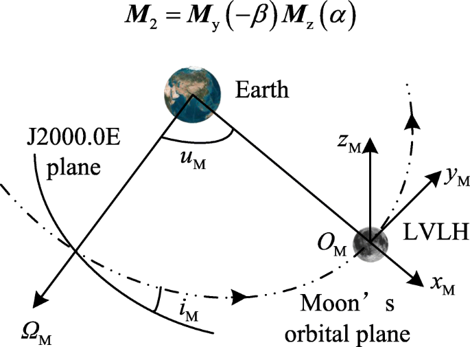
The drawing of the moon-centric LVLH coordinate system
$$ {\mathrm{M}}_1={\mathrm{M}}_{\mathrm{z}}\left({u}_{\mathrm{M}}\right){\mathrm{M}}_{\mathrm{y}}\left({i}_{\mathrm{M}}\right){\mathrm{M}}_{\mathrm{z}}\left({\Omega}_{\mathrm{M}}\right) $$(3)

And the two spherical angles α and β are defined in the moon-centric LVLH coordinate system as shown in Fig. 2. As thus, the free-return orbit’s perilune point vector just needs a matrix in Eq. (4) to rotate a z-y type Euler angle from the moon-centric LVLH coordinate system.

The drawing of the two spherical angles to locate the perilune point vector
So, the perilune position vector in the moon-centric LVLH coordinate system is shown in Eq. (5). Here, rprl is the radius value of the free-return orbit’s perilune and has a normal constant for follow-up lunar orbit insertion.
Step 2: a spherical angle γ is applied to describe the free-return orbit’s velocity vector at the time of perilune as shown in Fig. 3. Based on the Step 1, its velocity vector just needs an additional elementary x type of Euler angle rotation from the moon-centric LVLH coordinate system. The whole rotation matrix with a z-y-x type of Euler angles rotation is shown as Eq. (6).
Fig. 3 
The drawing of the spherical angle to describe the perilune velocity vector
$$ {\mathrm{M}}_3={\mathrm{M}}_x\left(\gamma \right){\mathrm{M}}_{\mathrm{y}}\left(-\beta \right){\mathrm{M}}_{\mathrm{z}}\left(\alpha \right) $$(6)

Assuming a confirmed perilune time tprl has been designed for lunar orbit insertion and follow-up lunar surface descent, and as mentioned the radius value of the free-return orbit’s perilune point has a normal constant. There are four elements are independent: the absolute value of perilune velocity vprl and the three Euler angles (i.e. α, β, and γ). Thus, the four independent design variables at the time of perilune can describe an exclusive circumlunar free-return orbit. The values of vprl is related to the radius value of the perilune point rprl and the orbit’s eccentricity eprl in the moon-centric LVLH coordinate system as shown in Eq. (7).
Here, μM is the lunar gravitational constant using 4.902801056 × 10¹² m3/s2 in LP165P model. For a free-return orbit with a low perilune altitude, its eccentricity eprl is greater than 1 and less than 2, so the initial value of vprl is about 2.55 × 10³ m/s. In addition, both the values of α and β are close to zero, and the value of γ is close to 180 deg. [7].
Two-Segment Numerical Integration Strategy
As the reason that the free-return orbit is quiet sensitive mentioned in section 3.1, this paper presents a method to divide the free-return orbit into two segments to reduce the instability as shown in Fig. 4. One obtains the orbital elements at the time of trans-lunar injection from perilune via a negative numerical integration manner, and the other segment obtains the orbital elements at the time of re-entry from perilune via a positive numerical integration manner. It is a flexible use of the multi-point correction scheme, and is similar to the multiple shooting methodologies for a long-time flight and sensitive transfer orbit design problem [26].

The drawing of the two-segment integration strategy
The skipping re-entry path angle at the earth’s atmosphere interface is not simple and direct to compute. Therefore, the vacuum perigee is used here. A lunar returned orbit with a − 6° skipping re-entry flight path angle has a corresponding 51 km vacuum perigee altitude at 122 km [27].
Searching Model Applying SQP_snop
A general searching model applied SQP_snopt (Student Edition, 7.2–2008) [28] is established as follow:
The independent design variables are shown in Eq. (8).
The low and upper boundaries (i.e. l.b. & u.b.) of x are shown in Eq. (9).
The free-return orbit’s radiuses at the times of trans-lunar injection and vacuum perigee compose the equivalence constraints (i.e. e.c.) as shown in Eq. (10). Here, the superscript []∗ denotes the objective value, and the subscript “vcp” denotes vacuum perigee as mentioned in section 3.2.
The free-return orbit for maned lunar landing mission based on LEO rendezvous has two contained constraints: Firstly, the orbit’s inclination at the time of trans-lunar injection is close or equal to the former vehicle or space-station on LEO. On the other hand, the returned segment will not fly after lunar orbit insertion in a normal program. Here, a minimized optimization objective function is designed as shown in Eq. (11).
The free-return orbit is a six degree of freedom dynamics system, two of them are fixed at the time of perilune (i.e. the radius value rprl and the embedded true anomaly is zero). Four independent design variables are used to matching two equivalence constraints in Eq. (10) and one optimization objective function in Eq. (11). Therefore, the solution is not one and only.
Adaptive LEO-Phase Iteration Algorithm
The LEO’s inclination constraint in Eq. (2) can be matched by the optimization objective function in Eq. (11). The LEO’s RAAN constraint in Eq. (2) need the launch day-window of LEO vehicle to match. In order to satisfy the argument of latitude constraint in Eq. (2), an adaptive LEO-phase iteration algorithm is presented as shown in Eq. (12)
Here, TLEO is the LEO’s orbit period. \( {u}_{\mathrm{tli}}^{\mathrm{old}} \) is the argument of latitude of the free-return orbit in J2000.0 E at the time of trans-lunar injection, which is corresponding to the old time of perilune \( {t}_{\mathrm{prl}}^{\mathrm{old}} \), and \( {u}_{\mathrm{LEO}}^{\mathrm{old}} \) is the argument of latitude of LEO at the time of trans-lunar injection, and it is corresponding to \( {t}_{\mathrm{prl}}^{\mathrm{old}} \). λ is a Newton-downhill ratio, the choice between 0 and 1 can be made. A new free-return orbit’s elements can be calculated by a new time of perilune \( {t}_{\mathrm{prl}}^{\mathrm{new}} \) with the SQP_snopt optimization algorithm mentioned in section 3.3. The new arguments of latitudes \( {u}_{\mathrm{LEO}}^{\mathrm{new}} \) and \( {u}_{\mathrm{tli}}^{\mathrm{new}} \) of LEO and free-return orbit, respectively, at the times of trans-lunar injection are refreshed. The iteration process stops until \( {u}_{\mathrm{tli}}^{\mathrm{new}} \)matches \( {u}_{\mathrm{LEO}}^{\mathrm{new}} \) at the engineering requirement. The iteration algorithm stops, and the ultimate free-return orbit’s elements meet the objective phase of LEO rendezvous.
Results and Discussion
In this section, the method to design an adaptive LEO-phase free-return orbit is tested by numerical simulation. The results and discussion are displayed and summarized.
Problem Configuration
Assume that the time of perilune is set as January 1, 2025 00:00:00.000 in Gregorian universal coordinated time format (UTCG). The perilune altitude hprl is equal to 111 km (60 n.mi.), and it means rprl is equal to 1849.2 km is equivalent as the equator radius of the moon is equal to 1738.2 km. The equator radius of the earth is set up for 6378.137 km, therefore, two equality constraints in Eq. (10) are equivalent to rLEO= 6563.337 km (i.e. hLEO= 185.2 km, 100 n.mi.) and \( {r}_{\mathrm{vcp}}^{\ast } \)= 6429.137 km (i.e. \( {h}_{\mathrm{LEO}}^{\ast } \)= 51 km) [25]. The objective value iLEO is equal to 28.5 deg. (0.49742 rad) refer to Cape Kennedy [29]. The Runge-Kutta 7th–8th order adaptive-step integrator is adopted, and the initial step is set as 60 s. The maximum absolute and relative errors both are set as 1 × 10⁻¹¹, and the interpolation tolerance of searching the periapsis is set as 1 × 10⁻⁷. The simulation is coded by Visual C++ on a computer using Intel Core2–2.0 GHz CPU.
Process of SQP_snopt Searching FRO
Set the initial values of independent variables as mentioned in section 3.1. The iteration process of searching an objective orbital inclination of free return orbit is shown in Fig. 5. It costs about 1980 s for 30 iteration times until the nonlinear constraints and optimization function converge, respectively.

The iteration process of nonlinear constraints feasible value and optimization function
The free-return orbit’s elements are listed in Table 1. The iteration process shows that the proposed method has an excellent performance.
In addition, for testing the adaptive LEO-phase iteration algorithm in Eq. (12), suppose that the worst LEO-phase situation took place, the delta argument of latitude of the free-return orbit and LEO at the time of trans-lunar injection is set as 180 deg. as listed in Table 1. The bold-font denotes the important iteration values of argument of the latitude.
Process of Adaptive LEO-Phase Free-Return Orbit Iteration
As the worst situation assumed in the section 4.2, the iteration process of adaptive LEO-phase free-return orbits is listed in Table 2. The Newton-downhill ratio is set as 0.9 considering the convergence speed and consistency in this example. After three times iteration, the delta argument of latitude of the free-return orbit and LEO becomes 0.21 deg., so, we think it satisfies the engineering constraints. It proved to be effective that the proposed method searches an adaptive LEO-phase free-return orbit. The radius of the perigees of trans-lunar injection and vacuum perigee matching the equality constraints shows that the two-segment numerical integration strategy is convenient.
The values of the independent design variables of free-return orbit are listed in Table 3, which are so adjacent to the initial values mentioned in section 3.1 significantly, and it is the reason why the optimization model applying SQP_snop in section 3.3 has an advantage of fast convergence speed.
Conclusions
In this study, an adaptive LEO-phase free-return orbit design model applying SQP_snop optimization algorithm is investigated, which has an advantage of fast convergence speed due to the two-segment numerical integration strategy and the particular independent design variables. Then a simple iteration for designing adaptive LEO-phase FRO is proposed, a Newton-downhill ratio is employed to improve the robust capacity and convergence speed of the iteration process. Simulation results based on a high-precision dynamics model have demonstrated the effectiveness of this approach. It could be used in the future manned lunar missions based on LEO rendezvous.
References
Lunney G. Discussion of several problem areas during the Apollo 13 operation [C]. AIAA 7th Annual Meeting and Technical Display, Houston, Texas. 1970
Miele, A.: Theorem of image trajectories in earth moon space [J]. Acta Astronautica. 6(51), 225–232 (1960)
Schwaniger, A.J.: Trajectories in the earth-moon space with symmetric free-return properties [R]. In: NASA Technical Note D-1833 (1963)
Jesick, M., Ocampo, C.: Automated generation of symmetric lunar free-return trajectories [J]. J. Guid. Control. Dyn. 34(1), 98–106 (2011)
Egorov V A. Three-dimensional lunar trajectories [R]. NASA Technical Translation, F-504,1969
Farquhar, R.W.: Dunham D W. a new trajectory concept for exploration the earth’s geomagnetic tail [J]. J. Guid. Control. Dyn. 4(2), 192–196 (1980)
He, B.Y., Li, H.Y., Zhou, J.P.: Solution domain analysis of earth-moon quasi-symmetric free-return orbits [J]. Trans. Japan Soc. Aero. Space Sci. 60(4), 195–201 (2017)
Egorov, V.A.: Certain problems of moon flight dynamics [M]. International Physical Index Inc, New York (1958)
Tolson, R.H.: Geometrical characteristic of lunar orbits established from earth-moon trajectories [R]. NASA Technical Note D-1780, Washington DC (1963)
Penzo A P. An analysis of free-flight circumlunar trajectories [C]. AIAA Astrodynamicss conference, new haven, Connecticut, USA, August, 19–21. 1963
Dallas, S.S.: Moon-to-earth trajectories [C]. AIAA Astrodynamics Conference, New Haven (1963)
Gibson F T. Application of the matched conic model in the study of circumlunar trajectories [R]. NASA Project Apollo Working Paper No.1066. 1963
Peng, Q.B., Shen, H.X., Li, H.Y.: Free return orbit design and characteristics analysis for manned lunar mission [J]. Sci. China Technol. Sci. 54(12), 3243–3250 (2011)
Li, J.Y., Gong, S.P., Baoyin, H.X.: Generation of multi-segment lunar free-return trajectories [J]. J. Guid. Control. Dyn. 36(3), 765–775 (2013)
Wilson S W. A pseudostate theory for the approximation of three-body trajectories [C]. AAS/AIAA Astrodynamics Conference, AAS/AIAA Astrodynamics Conference, Santa Barbaba, 1970
Wilson, R.S., Howell, K.C.: Trajectory design in the sun-earth-moon system using lunar gravity assists. J. Spacecr. Rocket. 35(2), 191–198 (1998)
Byrnes, D.: Application of the pseudostate theory to the three body lambert problem [J]. J. Astronaut. Sci. 37, 221–232 (1989)
Ramanan, R.: Integrate algorithm for lunar transfer trajectories using a pseudo state technical[J]. J. Guid. Control. Dyn. 25(2), 946~952 (2002)
Luo, Q.Q., Yin, J.F., Han, C.: Design of earth-moon free-return trajectories [J]. J. Guid. Control. Dyn. 36(1), 263–271 (2013)
Zhang, H.L., Luo, Q.Q., Han, C.: Accurate and fast design algorithm for free-return lunar flyby trajectories [J]. Acta Astronautica. 102(5), 14–26 (2014)
Stanley, D., Cook, S., Connolly, J., et al.: NASA’s exploration system architecture study [R]. NASA-TM-2005-214062. In: November (2005)
Yan, H., Gong, Q.: High-accuracy trajectory optimization for a trans-earth-lunar mission [J]. J. Guid. Control. Dyn. 34(4), 1219–1227 (2011)
He, B.Y., Li, H.Y., Zhang, B.: Analysis of transfer orbit deviation propagation mechanism and robust design for manned lunar landing [J]. Acta Phys. Sin. 62(19), 91–98 (2013)
Yim, S.Y., Baoyin, H.X.: High latitude landing circumlunar free return trajectory design [J]. Aircraft. Engin. and Aeros. Techn. 87(4), 380–391 (2015)
Berry, R.L.: Launch window and trans-lunar orbit, lunar orbit, and trans-earth orbit planning and control for the Apollo 11 lunar landing mission [R]. AIAA 8th Aerospace Sciences Meeting, AIAA 70–0024, New York (1970)
Topputo, F.: On optimal two-impulse earth-moon transfers in a four-body model [J]. Celestial Mech. Dyn. Astr. 117(3), 279–313 (2013)
Shen, H.X., Zhou, J.P., Peng, Q.B., et al.: Point return orbit design and characteristics analysis for manned lunar mission [J]. Sci. China Technol. Sci. 55(9), 2561–2569 (2012)
Gill, P.E., Murray, W., Saunder, M.A.: SNOPT: an SQP algorithm for large-scale constrained optimization [J]. Siam J. Optim. 12(4), 979–1006 (2002)
Garn M, Qu M, and Chrone J, et al. NASA’s planned return to the moon: global access and anytime return requirement implications on the lunar orbit insertion burns [C]. AAS/AIAA Astrodynamicss Specialist Conference and Exhibit, August. 2008
Acknowledgements
This work was supported by the National Natural Science Foundation of China (Grant No. 11702330) and National Defense Science and Technology Innovation Special Zone Project.
Author information
Authors and Affiliations
Corresponding author
Additional information
Publisher’s Note
Springer Nature remains neutral with regard to jurisdictional claims in published maps and institutional affiliations.
Rights and permissions
About this article

Cite this article
He, By., Li, Hn. & Zheng, Aw. Adaptive LEO-Phase Free-Return Orbit Design Method for Manned Lunar Mission Based on LEO Rendezvous. J Astronaut Sci 66, 446–459 (2019). https://doi.org/10.1007/s40295-019-00182-3
Published:
Issue Date:
DOI: https://doi.org/10.1007/s40295-019-00182-3