Bed load prediction in gravel-bed rivers using wavelet kernel extreme learning machine and meta-heuristic methods

Abstract

The present study aims at developing a wavelet kernel extreme learning machine (WKELM) and meta-heuristic method, known as particle swarm optimization (PSO). PSO algorithm is employed in order to provide a desirable modeling by optimal determination of parameters attributed to WKELM. In order to confirm the ability of employed PSO-WKELM approach in solving the problem, a well-known kernel-based support vector machine (SVM) is applied to compare the obtained results. 890 data points from 19 gravel-bed rivers located in the USA were used to feed the utilized heuristic models. Three different scenarios were proposed; in the scenario 1, different combinations of parameters based on hydraulic characteristics were prepared, scenario 2 was developed using both hydraulic and sediment properties as model inputs of bed load transport, and lastly, the performance of employed PSO-WKELM approach for prediction of bed load transport with different range of median particle size was investigated. The obtained results confirmed the higher predictive potential of PSO-WKELM in comparison with SVM. Also, it was found that prediction of bed load transport with median particles size ranging from 1 to 1.4 mm led to more valid outcome. Performing the sensitivity analysis demonstrated the remarkable impact of the ratio of average velocity (V) to shear velocity (U*) in modeling process.

Introduction

A reliable estimation of bed load transport rate in gravel-bed rivers has become a focal point of research in recent years. It can influence the three-dimensional morphology of rivers, and as a result, various studies relating to fluvial geomorphology and management applications need prediction of bed load. Considering the importance of this phenomenon, numerous models have been formulated and also discussed by researches for gravel-bed rivers (Khorram and Ergil 2010; López et al. 2014; Hinton et al. 2018). Although these formulas provide acceptable results in some cases, the complicated nature of sediment transport in gravel-bed rivers led to large errors in prediction of bed load (Barry et al. 2004; Bathurst 2007). Recently, machine learning methods such as artificial neural networks (ANNs), support vector machine (SVM), adaptive neuro-fuzzy inference system (ANFIS) and genetic programming (GP) have been used as alternative approaches to reduce the uncertainty of sediment transport problems. Sasal et al. (2009) reported the accuracy of ANN in predicting bed load of alluvial rivers. Azamathulla et al. (2009) suggested ANFIS method as a flexible and more optimum technique for predicting bed load in Malaysian rivers. Kitsikoudis et al. (2014) utilized machine learning for estimating bed load transport in gravel-bed rivers and showed that the models derived from ANNs and ANFIS generated superior results in comparison with symbolic regression (SR). Roushangar and Koosheh (2015) assessed the capability of SVR method for modeling bed load transport in gravel-bed rivers with the aim of using genetic algorithm for selecting optimal parameters of SVR. In general, the quality and performance of machine learning methods are influenced by a correct setting of hyperparameters. Different optimization algorithms such as particle swarm optimization (PSO) have been implemented with machine learning methods for this purpose. Chau (2006) used a combination of ANN and PSO for stage prediction of river. Zanganeh et al. (2011) proposed an effective prediction method based on ANFIS coupled with PSO to estimate scour depth. Huang et al. (2017) confirmed the excellent generalization capability of PSO-SVM for prediction of groundwater level. Sahraei et al. (2018) used a least square support vector regression (LSSVR) in which the parameters of kernel functions are optimized by PSO for the estimation of bed material load.

The extreme learning machine (ELM) is a single-layer feed-forward neural network (SLFN) which was proposed as a fast and easy usage learning method (Huang et al. 2006). Taking into account the advantages, this algorithm has earned enormous popularity for providing the accurate solution in different hydraulic problems (Ebtehaj et al. 2016; Roushangar et al. 2018a, b). However, optimal performance of ELM is dependent on the correct selection of neurons in the hidden layer and the appropriate activation function. In order to overcome the problems of randomly assigning the weights and choosing the hidden layer in ELM, a new method termed as the kernel extreme learning machine (KELM) has been developed (Huang et al. 2012). Using the kernel function for determining the hidden layer feature mapping generates more stability and also higher performance for prediction purposes. Promising applications of KELM for prediction of local scour around bridge piers (Pal et al. 2014), prediction of daily global solar radiation from air temperatures (Shamshirband et al. 2015) and prediction of total organic carbon (TOC) in marine mud shale reservoirs (Zhu et al. 2018) have been reported.

To the best of our knowledge, despite the high performance, the KELM approach with wavelet kernel function has not been used for the prediction of sediment load. Keeping in mind specific characteristics and capabilities of WKELM and for the purpose of increasing the prediction level of this method, for the first time, the PSO-WKELM approach is used to predict the bed load transport rate of gravel-bed rivers. The models were proposed based on three scenarios with different input combinations. The present study also discusses the most influential parameters in predicting bed load transport rate using sensitivity analysis. The obtained results were compared with the results of some well-known equations.

Materials and methods

Study area

The compilation of field data by US Forest service in cooperation with other agencies is utilized in the present study. Dataset has complete records of channel geometry, and hydraulic characteristics consist of flow depth (y), width of channel (B), flow velocity (V), flow discharge (Q) and median diameter of sediment particles (D₅₀). More details of study site characteristics and overall information are available in King et al. (2004). In this study, dataset which were collected from 19 gravel-bed rivers and streams within the Snake river basin in Idaho (USA) is considered. It is worthy of mention that on all sites, the d₅₀ and d₉₀ of the surface material were larger than those of the subsurface material, indicating the presence of an armor layer which is the main characteristics of gravel-bed rivers. The width to depth ratio for all selected rivers and streams is greater than 10 and the Froude number not exceeding 1. In total, there are 890 data points with V 0.13–2.30 m/s, y 0.05–2.24 m, D₅₀ 0.31–37.20 mm and slope 0.00038–0.017. Some characteristics of selected rivers and streams are provided in Table 1.

Table 1 Characteristics of the selected rivers

Kernel extreme learning machine

Recently, the ELM learning algorithm with fast learning speed and better generalization capability has gained enormous popularity from an increasing number of researchers. In ELM, there is no need for tuning the initial parameters of hidden layer and almost all nonlinear piecewise continuous functions can be used as the hidden neurons. Therefore, for N arbitrary distinct samples $\{ x_{i} ,t_{i} | x_{i} \in R^{n} , t_{i} \in R^{m} ,i = 1, \ldots ,N\}$, the output function in ELM with L hidden neurons can be expressed as:

$$f_{L} \left( x \right) = \mathop \sum \limits_{i = 1}^{L} \beta_{i} h_{i} \left( x \right) = h\left( x \right)\beta ,$$

(1)

where $\beta = \left[ {\beta_{1} ,\beta_{2} ,\ldots ,\beta_{L} } \right]$ is known as the vector of the output weights between the hidden layer of L neurons and the output neuron, and $h\left( x \right) = \left[ {h_{1} \left( x \right) ,h_{2} \left( x \right) ,\ldots ,h_{L} \left( x \right)} \right]$ denotes the output vector of the hidden layer with regard to the input x, which maps the data from input space to the ELM feature space (Huang et al. 2006). In order to decrease the training error and improve the generalization capability of neural networks, the training error and the output weights need to be minimized simultaneously, that is

$${\text{Minimize:}}\;\|H_{\beta } - T \|, \|\beta\|$$

(2)

The least squares solution of (2) based on KKT conditions can be expressed as:

$$\beta = H^{\text{T}} \left( {\frac{1}{\rho } + HH^{\text{T}} } \right)^{ - 1} T ,$$

(3)

where is the hidden layer output matrix, is the regulation coefficient, and is the expected output matrix of samples. Then, the output function of the ELM learning algorithm is

$$f\left( x \right) = h\left( x \right)h^{\text{T}} \left( {\frac{1}{\rho } + HH^{\text{T}} } \right)^{ - 1} T ,$$

(4)

If the feature mapping h(x) is unknown and the kernel matrix of ELM based on Mercer’s conditions can be defined as follows,

$$M = HH^{\text{T}} : m_{ij} = h\left( {x_{i} } \right) h\left( {x_{j} } \right) = k\left( {x_{i} ,x_{j} } \right) ,$$

(5)

And thus, the output function f(x) of the kernel-based extreme learning machine can be written compactly as:

$$f\left( x \right) = \left[ {k\left( {x,x_{1} } \right), \ldots , K\left( {x,x_{N} } \right)} \right]\left( {\frac{1}{\rho } + M} \right)^{ - 1} T$$

(6)

where $M = HH^{\text{T}}$ and $k\left( {x ,y} \right)$ is the kernel function of hidden neurons of single hidden layer feed-forward neural networks (Huang et al. 2012).

Among the various traditional kernel functions which are given as follows, the RBF kernel is reported to perform better than other kernel functions (Haghiabi et al. 2017; Mehdipour and Memarianfard 2018).

Linear kernel:

$$K(x_{i} ,x_{j} ) = (x_{i} ,x_{j} )$$

(7)

Polynomial kernel:

$$K(x_{i} ,x_{j} ) = \left( {(x_{i} ,x_{j} ) + 1} \right)^{d}$$

(8)

RBF kernel:

$$K(x_{i} ,x_{j} ) = \exp \left( { - \left\| {x_{i} - x_{j} } \right\|^{2} /2\gamma^{2} } \right)$$

(9)

In this study, wavelet kernel function is utilized for simulation and performance analysis of KELM approach:

$$K(x_{i} ,x_{j} ) = \cos \left( {\omega \frac{{\left\| {x_{i} - x_{j} } \right\|}}{\alpha }} \right)\exp \left( { - \frac{{\left\| {x_{i} - x_{j} } \right\|}}{\beta }^{2} } \right)$$

(10)

The wavelet kernel estimates the non-stationary signal with high accuracy, which is impossible for traditional kernels. The wavelet function is orthonormal, which almost estimates any function in continuous space; thus, the generalization of wavelet KELM is improved.

Since the variable parameters of wavelet kernel function such as α, β and ω can considerably affect the accuracy of training process, particle swarm optimization (PSO) method is applicably administered to determine optimal WKELM parameters and also regulation coefficient parameter of ρ.

Particle swarm optimization

Particle swarm optimization (PSO) is inspired by the social behavior of birds trying to find their food in nature. The original form of this algorithm is founded on the communication and cooperation of the birds looking for food within an area (Eberhart and Kennedy 1995). The birds pursue the nearest one to the food and simultaneously using their previous experiences find the food (Kennedy and Eberhart 2001). The food can be found only in one point in the search area that the birds are not informed of. The actions of each solution are like birds, which is known as a particle in this algorithm. Each particle enjoys a merit value through optimizing the objective function. PSO first generates an initial random solution each of which has an n-dimensional position (X), where n is the number of decision variables. Furthermore, it allots a velocity vector (V) between the maximum and minimum admissible velocities to each particle. PSO requires defining some parameters with the aim of producing a new population for the next generation and has progress in terms of convergence. These parameters are inertia weight (w), inertia weight reduction factor (α), minimum inertia weight (w_min), personal and global acceleration values (c₁ and c₂) and maximum velocity reduction factor (β). In every generation, the personal (P_p, the best position which every single particle has ever had since the beginning to the current generation) and global (P_g, the best ever position among all particles) best particles are detected to update the population for the next iteration. The position of each particle can be improved using following equations:

$$V_{k + 1}^{i} = wV_{k}^{i} + c_{1} r_{1,k} (P_{k}^{p} - X_{k}^{i} ) + c_{2} r_{2,k} (P_{k}^{g} - X_{k}^{i} )$$

(11)

$$X_{k + 1}^{i} = X_{k}^{i} + V_{k + 1}^{i}$$

(12)

where w is suggested to be considered between 0.8 and 1.4, $r_{1,k}$ and $r_{2,k}$ are the random uniform numbers between zero and one, and k is the iteration number. The velocity values are limited to $\left[ { - V_{\text{max} } ,V_{\text{max} } } \right]$. In order to ensure the convergence of PSO to the optimal objective and either when there is no notable change in the value of objective function (Eq. 13) or after a certain number of generation the algorithm terminates,

$$\frac{{F_{\hbox{max} } - F_{\hbox{min} } }}{{F_{\hbox{min} } }} \le \varepsilon$$

(13)

In this study, developed PSO-WKELM approach was codified in MATLAB software.

Support vector machine

Many researches have been done in various fields of engineering using support vector machine. Therefore, only a brief summary of the employed SVM model called ɛ-SVM is presented here. The original SVM algorithm was proposed by Vapnik (1995). It is assumed that for dataset $\left\{ {x_{i} ,y_{i} } \right\}$, the nonlinear function for SVM regression can be given as:

$$f(x) = W\varphi (x) + b$$

(14)

So the main issue is to find the form of the f(x) function with high deviation (ɛ) from target (y_i), and it should be as flat as possible at the same time. This function is accessible by training the SVM model on a dataset, which includes a process for continuously optimizing the error function. Based on the definition of this error function, two examples of SVM models are known: (a) SVM regression models of the first type that are known as v-SVM models; (b) second type of SVM regression models, which are ɛ-SVM models based on minimizing the distance of all data points by determining the optimal hyperplane. In this study, the ε-SVM model was used due to its wide application in regression problems. For this model, the error function is defined as follows.

$$\frac{1}{2}W^{\text{T}} W + C\sum\limits_{i = 1}^{N} {\xi_{i} + X\sum\limits_{i = 1}^{N} {\xi_{i}^{*} } }$$

(15)

The error function should be minimized according to the following constraints:

$$\begin{aligned} & W^{\text{T}} \phi (X_{i} ) + b - y_{i} \le \varepsilon + \xi_{i}^{*} \\ & y_{i} - W^{\text{T}} \phi (X_{i} ) = b \le \varepsilon + \xi_{i}^{*} \\ & \xi_{i} ,\xi_{i}^{*} \ge 0,i = 1, \ldots ,N \\ \end{aligned}$$

(16)

where C and ɛ are, respectively, the capacity constant and error-intensive zone, the vector W is known as the weight factor, and W^T is the transposed form of it, ξ_i and ξ_i* are called Slack Variables, b is the bias, and ϕ is the kernel function. In this study, the commonly used radial basis function was utilized as the kernel trick of the support vector machine.

Traditional approaches

Owing to complicated nature of sediment transport, a variety of numerical models have been formulated and verified. The efficiency of developed formulas depended on their theoretical backgrounds, methods of sampling and mathematical approaches (Yang 1996). These formulas have been developed based on different concepts and approaches such as shear stress, probabilistic and stream power approaches (Khorram and Ergil 2010). Furthermore, equal mobility approach has been applied for derivation of some formulas (Parker 1990). Under conditions of equal mobility, the bed load transport rate could be computed from a single representative grain diameter such as the median size, D₅₀. In this study, bed load formulas of Parker et al. (1982), Wilcock (2001), Rottner (1959) and Engelund and Hansen (1972) were used as well-known formulas to calculate bed load transport rate and moreover, to compare with predicted values by PSO-WKELM models. Selected bed load transport equations are given in Table 2.

Table 2 Selected traditional formulas for predicting bed load

Where U*: shear velocity, θ and θ_cr: shields’ and critical shields’ parameters for initiation of motion, _s: density of sediment, G_s: relative density of sediment, τ₀ and τ_cr: shear and critical shear stress at the bed, R_h: hydraulic radius, V_av: average velocity, d_s: diameter of particles and q_b: bed load transport rate per unit width.

Performance criteria

In order to evaluate how the hybrid models of PSO-WKELM perform, three statistical criteria, namely the root-mean-square error (RMSE), correlation coefficient (R) and Nash–Sutcliffe efficiency (NSE), are used. The RMSE is applied to exhibit the accuracy of modeling process, which generates a positive value by squaring the errors. The RMSE grows from zero for excellent predictions over large positive values as the differences between predictions and observations become increasingly large. Furthermore, R and NSE are well-known correlation-based measures which have been used in water resources modeling. Clearly, a high values for R and NSE (up to one) and small value for RMSE denote high performance of model. Statistical parameters are formulated as follows:

$$R = \frac{{\sum\nolimits_{i = 1}^{N} {(X_{i} - \bar{X}) \times (Y_{i} - \bar{Y})} }}{{\sum\nolimits_{i = 1}^{N} {(X_{i} - \bar{X})^{2} \times (Y_{i} - \bar{Y})^{2} } }}$$

(21)

$${\text{RMSE}} = \sqrt {\sum\limits_{i = 1}^{N} {\frac{{(X_{i} - Y_{i} )^{2} }}{N}} }$$

(22)

$${\text{NSE}} = 1 - \frac{{\sum\nolimits_{i = 1}^{N} {(X_{i} - Y_{i} )^{2} } }}{{\sum\nolimits_{i = 1}^{N} {(X_{i} - \overline{{X_{i} }} )^{2} } }}$$

(23)

where N represents the number of data, X_i and Y_i are the observed bed load and predicted bed load.

Data preparation

For the purpose of predicting bed load transport rate due to training and testing goals, datasets were separated into two parts. Considering that the data compilation includes datasets coming from various streams and rivers, for all cases, 75% of data from each river were divided for training the model and remaining 25% were used for test purposes. As a result, there are 612 measurements for training and 278 measurements for testing. Input and output variables were normalized in the intervals of 0.1 and 0.9 with the aim of eliminating their dimensions and enhancing the accuracy of the modeling process.

Input parameters

Finding the optimum input configuration is of essential importance throughout the modeling process. For determining the input combinations, various independent variables based on hydraulic conditions such as Froude number, ratio of flow depth to channel width (y/B), bed slope of the channel (S₀) and ratio of average velocity to shear velocity (V/U*) were defined. Additionally, some other parameters based on sediment characteristic were entered in modeling process including particle mobility parameter ($\theta = U_{*}^{2} /(G_{\text{s}} - 1)gD_{50}$), depth-particle size ratio (y/D₅₀), particle parameter ($D_{*} = D_{50} ((G_{\text{s}} - 1)g/\upsilon^{2} )^{1/3} )$), transport stage parameter ($T = \theta^{\prime } - \theta_{\text{cr}} /\theta_{\text{cr}}$), where θ′ refers to mobility parameter related to grain roughness and θ_cr is the shields’ critical shear stress. Following parameters were selected after trial-and-error process to describe the bed load transport rate (Bhattacharya et al. 2007; Pektaş 2015).

$$Q_{b} = f\left( {Fr,\frac{V}{{U_{*} }},\frac{y}{B},S_{0} ,\theta ,\frac{y}{{D_{50} }},D_{*} ,T} \right)$$

(21)

Different combinations of mentioned parameters were developed, and by carrying out a large number of trials, the best models were selected.

PSO-WKELM modeling development

The performance of WKELM approach is dependent on good setting of user-defined parameter of $\rho$ and kernel parameters. For this reason, PSO was incorporated in the WKELM algorithm for bed load transport estimation. The detail steps can be summarized as follows:

• Step 1: Initialize particle population including initial velocity V and position X; assign number of iteration, population size, inertial weight and acceleration constant.

• Step 2: Compute the fitness of each particle; Nash–Sutcliffe efficiency (NSE) was used as the fitness function to conduct particle population in finding the best solution.

• Step 3: Update the values of P_p and P_g in consonance with the fitness.

• Step 4: Update the velocity and position of each particle in consonance with P_p and P_g.

• Step 5: Select the optimum values of user-defined parameter of and kernel parameters at the maximum number of iterations and implement the best WKELM prediction model using the optimum solution. The flowchart of WKELM model optimization is presented in Fig. 1.

  Fig. 1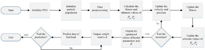

  

  Flowchart of WKELM model optimization based on PSO algorithm

Proposed scenarios

Some limitations including expensive and time-consuming procedure inhibited the collection of bed load transport data. In this regard, scenario 1 was defined in which the parameters based on flow characteristics were taken into account as input data. It would be more useful in some cases, based on the fact that there could be only flow characteristics as available data. On the other hand, in scenario 2, for predicting the bed load transport rate in gravel-bed rivers, several models were developed according to the flow condition and particle’s features. Furthermore, the characteristic particle sizes in the bed load transport can considerably change both in time and space. This variability can reduce the accuracy of the sediment transport prediction possibilities. Scenario 3 was developed to investigate the prediction capability of PSO-WKELM in different intervals of median particle sizes.

Results and discussion

The results of PSO-WKELM models are shown in Table 3. The model with input parameters of Froude number (Fr) and ratio of average velocity to shear velocity (V/U*) which had a test R of 0.825, NSE = 0.670 and RMSE = 0.040 was selected as the best model of scenario 1. It can be noticed from the obtained results that replacing y/B instead of S_f in models with three input variables can improve the accuracy of modeling. However, based on the results, it could be stated that the models established with only flow features are not so accurate. In scenario 2, different combinations of input variables were developed after a trial-and-error process according to flow and sediment properties. For this scenario, the combination of Fr, V/U* and T led to the best result (R = 0.934, NSE = 0.870 and RMSE = 0.025). As can be seen from the results, Fr and V/U* had dominant role in the prediction of bed load transport rate. On the other hand, for the models with three input parameters, introducing T instead of y/D₅₀ improved the global average accuracy. It is also observed that using three inputs ensured the best performance of PSO-WKELM and increased number of inputs did not have any effect on improving the obtained results. Actually, this method constructs necessary input–output mapping using the dataset and uses the minimum required parameters of modeling. The PSO-WKELM approach demonstrated higher precision than SVM for all developed models, and a detailed comparison of the overall performance confirmed the undesirable results of SVM for proposed models. The scatter plots of predicted relative bed load versus observed values for optimal model are depicted in Fig. 2. Due to high dispersion of data in low sediment transport rate and in order to compare the obtained results in a better way, the scatter plots are shown on logarithmic scale. It can be clearly noticed from Fig. 2 that SVM overestimated the bed load and PSO-WKELM presented better predictive performance. Optimization process of kernel parameters showed that variation of parameter ω which controls the kernel shape was from 0.4826 to 10 and as well as the values of α and β were optimized in the ranges of 2.2456–9.1158 and 0.007–0.16, respectively. Statistical parameters of traditional approaches for predicting bed load transport rate are presented in Table 4. Proposed formulas obviously presented poor results which caused unreliability of traditional methods in predicting bed load. It is worthy of mention that the notably low generalization regarding the traditional approaches is due to the restrictions of the ranges of the parameters tested in laboratory conditions, and in consequence, not all the physical properties behavior of the bed load transport can be exactly extracted. This caused an inaccuracy and also negative values of NSE in predicting bed load transport rate of natural rivers which means that the predictor is worse than average base models.

Table 3 Results of PSO-WKELM and SVM approaches for prediction of the bed load transport rate

Fig. 2

Comparison of observed and predicted bed load transport rate for optimal model

Table 4 Results of traditional approaches

In order to compare the accuracy and also the capability of the wavelet and RBF kernel functions in performance of PSO-KELM, model with input parameters of Fr, V/U* and T as the best combination was analyzed by using mentioned kernel functions. The obtained results revealed the superior performance of wavelet kernel function. However, the RBF kernel function showed more flexibility and faster training speed due to its fewer variables and simple structure in comparison with wavelet function. In case of RBF kernel, γ stands for the optimal width of kernel function. Great values of γ let kernel-based approaches to have a strong impact over a large area. Comparison of results from employed algorithms showed that KELM with fewer values of γ gives more accurate outcomes for developed model. Accordingly, there was no linear relation and definite pattern between γ and performance criteria and possibly it can show different behaviors for different approaches and inputs. Figure 3 demonstrates the optimization process of KELM approach with RBF and wavelet kernel functions and also depicts the statistic parameter of NSE via γ values with the aim of comparing the impact of RBF kernel parameter of γ on performance of employed algorithms for testing set of best model.

Fig. 3

Optimization process of KELM with wavelet and RBF kernel functions and statistic parameter of NSE via values of RBF kernel parameter of γ

One of the main reasons for the difficulty of bed load estimation in gravel-bed rivers is the variation of bed material size (Zhang et al. 2010). In this part of study, it was attempted to depict the effect of bed material size in prediction process of bed load transport rate. The accuracy of best input combination in different intervals of median diameter of sediment particles (D₅₀) was investigated based on large number of trial-and-error procedure, and the results are listed in Table 5. According to prediction results of PSO-WKELM approach, it can be seen that prediction of bed load transport rate with the median diameters of sediment particles (D₅₀) ranging from 1 to 1.4 mm led to significant outcomes of R = 0.991, NSE = 0.982 and RMSE = 0.015. Obtained results revealed that PSO-WKELM presents better performance in prediction of bed load transport with median particle size less than 2 mm which includes more than 80% of utilized data. However, incensement of flow rate caused movement of coarser particles which play armor layer role in gravel-bed rivers (Wang and Liu 2009). This caused a sudden scouring of finer subsurface material and developed a complicated hydraulic condition which reduced the prediction accuracy of PSO-WKELM dramatically (NSE = 0.073) for transportation of bed load with median particles greater than 2 mm. Different effective parameters in bed load transport should be considered at various flow conditions. In order to enhance the prediction level of bed load transport with coarser bed material (median particles greater than 2 mm), other parameters were considered as inputs with Froude number and ratio of average velocity to shear velocity. Obtained results showed that adding the shields number (θ) instead of transport stage parameter (T) improved the global average accuracy in NSE = 0.743. It seems shields number as a criterion for incipient motion is the most important parameter since floods may initiate bed load transport by moving coarser bed material. Figure 4 shows the comparison of PSO-WKELM and SVM methods in prediction of bed load transport rate with coarser material with input parameters of Fr, V/U* and θ.

Table 5 Results of employed approaches for prediction of bed load in different intervals of median particles size

Fig. 4

Comparison of the performance of PSO-WKELM and SVM methods in prediction of bed load transport rate with coarser material with input parameters of Fr, V/U* and θ

Sensitivity analysis

To derive the most dominant parameters for prediction of the bed load transport rate by PSO-WKELM, a sensitivity analysis was carried out. For investigating the influence of each independent parameter, the best model with three inputs was selected, and then, one of the input parameters was eliminated, and the POS-WKELM model was prepared again. Eliminating one of the input parameters could affect the performance of employed method. NSE performance criteria were used as indication of the importance of each parameter. The results of the sensitivity analysis are depicted in Fig. 5. ΔNSE denotes the percentage of reduction values to Nash–Sutcliffe efficiency which corresponded to each eliminated parameter. According to the results, the absence of the V/U* led to a dramatic decrease in terms of NSE value and reduces the performance of modeling, so it can be stated that the parameter V/U* plays a significant role in predicting the bed load transport rate of gravel-bed rivers.

Fig. 5

Obtained results of sensitivity analysis

Conclusion

The present study evaluates the functionality of generalized WKELM approach for prediction of the bed load transport rate in gravel-bed rivers. For the purpose of improving the overall performance, this technique was coupled with PSO algorithm to determine optimal parameters for WKELM models. Different input combinations were developed based on three scenarios. The obtained results confirmed the superiority of scenario 2 in quantification of bed load transport rate. Model including parameters Fr, V/U* and T with the highest level of R (0.934), NSE (0.870) and lowest value of RMSE (0.025) for test series showed more precise and robust prediction ability in comparison with SVM. The proposed input combination was used to predict the bed load transport in different intervals of median particles size. The results showed that the bed load transport in the intervals of 1 to 1.4 mm generated better predictive ability with NSE = 0.982. The present study indicated that the V/U* parameter had dominant role in predicting the bed load transport rate. There was also a discussion of the capability of traditional approaches for predicting the sediment load. The results demonstrated that these formulas suffered extremely from poor results due to their limitations of ranges of input–output parameters and also complicated conditions which govern sediment transport in natural gravel-bed rivers. Obtained results extracted from the sensitivity analysis revealed that the ratio of average velocity to shear velocity is the most influential parameter in prediction of bed load. However, it should be pointed out that utilized PSO-KELM approach is data sensitive, so it is recommended to carry out more studies using more filed data to confirm the merits of proposed models.

References

Azamathulla HM, Chang CK, Ghani AA, Ariffin J, Zakaria NA, Hasan ZA (2009) An ANFIS-based approach for predicting the bed load for moderately sized rivers. J Hydro-Environ Res 3(1):35–44
Barry JJ, Buffington JM, King JG (2004) A general power equation for predicting bed load transport rates in gravel bed rivers. Water Resour Res 40(10):W10401
Bathurst JC (2007) Effect of coarse surface layer on bed-load transport. J Hydraul Eng 133(11):1192–1205
Bhattacharya B, Price RK, Solomatine DP (2007) Machine learning approach to modeling sediment transport. J Hydraul Eng 133(4):440–450
Chau KW (2006) Particle Swarm Optimization training algorithm for ANNs in stage prediction of Shing Mun River. J Hydrol 329(3–4):363–367
Eberhart RC, Kennedy J (1995) A new optimizer using particle swarm theory. In: Proceedings of the sixth international symposium on micro machine and human science, vol 1, Nagoya, Japan, pp 39–43
Ebtehaj I, Bonakdari H, Shamshirband S (2016) Extreme learning machine assessment for estimating sediment transport in open channels. Eng Comput 32(4):691–704
Engelund F, Hansen E (1972) A monograph on sediment transport in alluvial streams. Teknisk Forlag, Copenhagen
Haghiabi AH, Azamathulla HM, Parsaie A (2017) Prediction of head loss on cascade weir using ANN and SVM. ISH J Hydraul Eng 23(1):102–110
Hinton D, Hotchkiss RH, Cope M (2018) Comparison of calibrated empirical and semi-empirical methods for bedload transport rate prediction in gravel bed streams. J Hydraul Eng 144(7):04018038
Huang GB, Zhu QY, Siew CK (2006) Extreme learning machine: theory and applications. Neurocomputing 70(1):489–501
Huang GB, Zhou H, Ding X, Zhang R (2012) Extreme learning machine for regression and multiclass classification. IEEE Trans Syst Man Cybern B Cybern 42(2):513–529
Huang F, Huang J, Jiang SH, Zhou C (2017) Prediction of groundwater levels using evidence of chaos and support vector machine. J Hydroinform 19(4):586–606
Kennedy J, Eberhart R (2001) Particle Swarm Optimization. Academic Press, San Francisco
Khorram S, Ergil M (2010) Most influential parameters for the bed-load sediment flux equations used in alluvial rivers 1. J Am Water Resour Assoc 46(6):1065–1090
King JG, Emmett WW, Whiting PJ, Kenworthy RP, Barry JJ (2004) Sediment transport data and related information for selected coarse-bed streams and rivers in Idaho. General technical report RMRS-GTR-131, vol 131. Fort Collins, US Department of Agriculture, Forest Service, Rocky Mountain Research Station
Kitsikoudis V, Sidiropoulos E, Hrissanthou V (2014) Machine learning utilization for bed load transport in gravel-bed rivers. Water Resour Manag 28(11):3727–3743
López R, Vericat D, Batalla RJ (2014) Evaluation of bed load transport formulae in a large regulated gravel bed river: the lower Ebro (NE Iberian Peninsula). J Hydrol 510:164–181
Mehdipour V, Memarianfard M (2018) Ground-level O3 sensitivity analysis using support vector machine with radial basis function. Int J Environ Sci Technol. https://doi.org/10.1007/s13762-018-1770-3
Pal M, Singh NK, Tiwari NK (2014) Kernel methods for pier scour modeling using field data. J Hydroinform 16(4):784–796
Parker G (1990) Surface-based bedload transport relation for gravel rivers. J Hydraul Res 28(4):417–436
Parker G, Klingeman PC, McLean DG (1982) Bedload and size distribution in paved gravel-bed streams. J Hydr Eng Div ASCE 108(4):544–571
Pektaş AO (2015) Determining the essential parameters of bed load and suspended sediment load. Int J Global Warm 8(3):335–359
Pitlick J, Cui Y, Wilcock P (2009) Manual for computing bed load transport using BAGS (Bedload Assessment for Gravel-bed Streams) Software. General technical report RMRS-GTR-223, vol 223. Fort Collins, US Department of Agriculture, Forest Service, Rocky Mountain Research Station
Rottner J (1959) A formula for bed load transportation. Houille Blanche 14(3):285–307
Roushangar K, Koosheh A (2015) Evaluation of GA-SVR method for modeling bed load transport in gravel-bed rivers. J Hydrol 527:1142–1152
Roushangar K, Alipour SM, Mouaze D (2018a) Linear and non-linear approaches to predict the Darcy–Weisbach friction factor of overland flow using the extreme learning machine approach. Int J Sediment Res. https://doi.org/10.1016/j.ijsrc.2018.04.006
Roushangar K, Alizadeh F, Nourani V (2018b) Improving capability of conceptual modeling of watershed rainfall–runoff using hybrid wavelet-extreme learning machine approach. J Hydroinform 20(1):69–87
Sahraei S, Alizadeh MR, Talebbeydokhti N, Dehghani M (2018) Bed material load estimation in channels using machine learning and meta-heuristic methods. J Hydroinform 20(1):100–116
Sasal M, Kashyap S, Rennie CD, Nistor I (2009) Artificial neural network for bedload estimation in alluvial rivers. J Hydraul Res 47(2):223–232
Shamshirband S, Mohammadi K, Chen HL, Samy GN, Petković D, Ma C (2015) Daily global solar radiation prediction from air temperatures using kernel extreme learning machine: a case study for Iran. J Atmos Sol Terr Phys 134:109–117
Vapnik V (1995) The nature of statistical learning theory. Data mining and knowledge discovery. Springer, Berlin, pp 1–47
Wang T, Liu X (2009) The breakup of armor layer in a gravel-bed stream with no sediment supply. In: Xiao C, Liang X, Zhang F, Feng B, Xie S (eds) Advances in water resources and hydraulic engineering. Springer, Berlin, pp 919–923
Wilcock PR (2001) Toward a practical method for estimating sediment-transport rates in gravel-bed rivers. Earth Surf Process Landf 26(13):1395–1408
Yang CT (1996) Sediment transport: theory and practice. McGraw-Hill, Singapore
Zanganeh M, Yeganeh-Bakhtiary A, Bakhtyar R (2011) Combined Particle Swarm Optimization and fuzzy inference system model for estimation of current-induced scour beneath marine pipelines. J Hydroinform 13(3):558–573
Zhang K, Wang ZY, Liu L (2010) The effect of riverbed structure on bed load transport in mountain streams. Mouth 6:3
Zhu L, Zhang C, Zhang C, Zhou X, Wang J, Wang X (2018) Application of multiboost-KELM algorithm to alleviate the collinearity of log curves for evaluating the abundance of organic matter in marine mud shale reservoirs: a case study in Sichuan Basin, China. Acta Geophys 66:1–18
Acknowledgements
The authors would like to extend their appreciation to the US Forest Service and other agencies for providing extensive database to carry out this research.
Author information
Authors and Affiliations
Corresponding author
Additional information
Editorial responsibility: M. Abbaspour.
Rights and permissions
About this article
Cite this article
Roushangar, K., Shahnazi, S. Bed load prediction in gravel-bed rivers using wavelet kernel extreme learning machine and meta-heuristic methods. Int. J. Environ. Sci. Technol. 16, 8197–8208 (2019). https://doi.org/10.1007/s13762-019-02287-6
Received:
Revised:
Accepted:
Published:
Issue Date:
DOI: https://doi.org/10.1007/s13762-019-02287-6