
Abstract
An increase in the applications of renewable-based energy resources in the radial distribution network has led to many uncertainties in the existing system which affects the stable operation of the power systems. The issues regarding the generation uncertainty associated with wind energy and photovoltaic (PV) systems along with load demand uncertainties are considered in this research for the evaluation of the maximum penetration level of renewable energy resources. The nodes which are less voltage stable are considered as the most suitable locations for distributed generations (DGs) placement from voltage stability viewpoint. For identification of DGs locations, a voltage stability index–continuous power flow-based algorithm has been proposed. To analyze the effect of large penetration level of wind and PV on voltage profile, power losses and system voltage stability of the radial distribution network, a probabilistic-based approach has been adopted. It is observed from simulation results that the penetration level limit depends upon the type of DGs connected to the radial distribution network. Usually the integration of DGs reduces the power losses in the network; however, as penetration level increases, the power losses begin to increase. The detailed mathematical model of wind and PV sources has been utilized. The Hong’s 2m + 1 point estimation method combined with Cornish–Fisher expansion has been adopted in this paper for probabilistic studies. The effectiveness of the proposed method has been validated through IEEE 33 and 69 node radial distribution test network for various scenarios. The results obtained are verified and compared with benchmark Monte Carlo simulation technique.
1 Introduction
Due to advancement in the renewable-based generation technologies, a rapid development and integration of these energy resources into existing power networks is being witnessed in recent years. The energy outputs from renewable energy sources, i.e., wind and solar photovoltaic (PV), are random and stochastic in nature and depends upon weather conditions. With large penetration level of renewable DGs into distribution network, the uncertainties associated with generation and loads had significantly influenced system voltage stability [1]. For studying uncertainties associated with the power system, probabilistic load flow (PLF) method is one of the best known tools. Probabilistic load flow methods are broadly categorized as Monte Carlo simulation (MCS) and analytical methods. MCS is a traditional method which provides more accurate results as compared to other analytical methods. However, thousands of iterations are required to simulate that are extremely time consuming and are unsuitable for real-time applications [2]. To reduce the simulation time analytical methods such as point estimation method (PEM) [3, 4], Cumulants method [5], Cumulants and Gram–Charlier expansion [6], Cumulants and Cornish–Fisher expansion [7] are used for probabilistic load flow (PLF) studies. DG integration in distribution network has several benefits such as reduction in system power loss, reduced emission, increase in system reliability, improved power quality and deferral of transmission upgrades. Due to the small capacity of DGs in comparison with central power plant, its impacts are minor if the penetration level (1–5%) is low. However, if the penetration level of DGs reaches the 40% level, the DGs impact cannot be neglected [8]. In the literature, the system voltage constraint is taken as one of the criteria for finding the maximum penetration level of DGs [9,10,11,12,13,14].
The voltage sensitivity-based analytical method is used to determine the maximum penetration limit of DGs in the distribution network without violating the voltage constraints [9]. The maximum penetration of solar PV-based DGs with various time-varying load models, i.e., residential, industrial and commercial, were investigated [10]. It was observed that penetration limit depends upon the types of load and system size. The effect of PV locations on maximum penetration limits was studied [11], and it was found that in 86% of cases the maximum penetration level could go beyond 30%. However, the voltage violations were observed in low voltage (LV) distribution network due to the high penetration of rooftop solar PV penetration [12]. The eigenvalue analysis was performed to determine the maximum penetration of grid connected solar PV system [13]. A literature review on solar PV penetration limit due to voltage violations in LV network was done in [14]. The review reveals the fact that high penetration level can be achieved in LV network as compared to medium voltage (MV) network. In order to solve the problem of voltage violations in large solar PV integrated network, the on-load tap changer (OLTC) fitted transformer could be the potential solution [15]. It is observed that installation of energy storage systems (ESS) at PV location is capable to raise the PV penetration level [16, 17]. It is observed from literature survey that very little work has been reported on maximum penetration limit of wind energy. The penetration limit of wind energy in the distribution network can be increased by implementing active network control such as generation curtailment, reactive power absorption with coordinated OLTC control [18]. The analytical techniques with the use of deterministic load flow are usually employed to evaluate the maximum penetration limit of DGs. Due to the uncertainty associated with the power output of DGs and system load demand, the probabilistic-based methods are required to evaluate the accurate estimation of the maximum penetration level of DGs. The MCS-based probabilistic approach is made use of to evaluate the maximum penetration limit of DGs in LV network [19, 20]. The impact on voltage stability due to the large penetration of DGs in the distribution networks is less evaluated. The voltage stability-based P–V/Q–V curve method is explored along with MCS and empirical distribution function (EDF) in the radial distribution network to determine maximum penetration level of DGs [21]. The probabilistic continuous power flow (CPF) method with load demand variation is used to determine the probabilistic voltage stability margins [22]. The stochastic response surface method (SRSM) is adopted to determine the probabilistic load margins in [23]. In [24], the authors have investigated the static voltage stability margins in the distribution network using two-point estimation method (2PEM) and CPF technique. Moreover, the probability density function (PDF) of the critical voltage stability is evaluated using Cornish–Fisher series expansion. In [25], the variations in load demand of the system are taken as hyper-cone model. The intersection point of the transfer limit surface and the loading hyper-cone is utilized to evaluate the worst case loading. In [26], the assessment of voltage stability margins is done using probabilistic load flow considering random variations in load demands, generation unit unavailabilities and topological variations. In [27], for determining the probabilistic voltage stability margin, the maximum entropy method is utilized. The probabilistic load flow for the unbalanced distribution network is proposed in [28] considering uncertainties of load and wind power generation.
In order to investigate the maximum penetration level of DGs in the radial distribution network, the researchers have taken either wind energy or solar PV-based DGs. But evaluation of the penetration limit of hybrid DGs based on a combination of solar PV and wind on the distribution network has not been investigated so far as per author’s knowledge. The deterministic load flow is usually employed to assess the maximum penetration of DGs. Due to uncertainty associated with power output of DGs and system load, for accurate estimation of maximum penetration level probabilistic approaches are required. Although some probabilistic studies have been investigated with MCS for determining maximum DG penetration, no studies have been investigated with analytical methods such as point estimation method as per author’s knowledge. In probabilistic load flow with non-Gaussian input random variables, Cornish–Fisher expansion has found better performance than the Gram–Charlier expansion for obtaining PDF and CDF of output variables [29]. In this paper, Hong’s 2m + 1 point estimation method is explored for the probabilistic load flow study [30], whereas Cornish–Fisher expansion has been utilized for obtaining the PDF and CDF of output variables. Voltage stability index (VSI) is used to obtain a suitable location of DGs from voltage stability point of view. To analyze the effect of large penetration of renewable DGs, four different scenarios are taken into account. The rest of the paper is organized as follows: Sect. 2 elaborates modeling of renewable energy sources and system load. Section 3 explores Hong’s 2m + 1 point estimation method coordinated with Cornish–Fisher expansion, MCS method and VSI that has been considered. Section 4 describes the proposed algorithm for investigation of probabilistic voltage stability for different load levels. In Sect. 5, case study is performed on 33-node radial distribution test network. Finally, Sect. 6 concludes the research work.
2 Modeling of Renewable Energy Sources and Load
2.1 Photovoltaic Modeling
The uncertainty associated with solar irradiance can be modeled as a beta probability density function (PDF) [31]. The PDF for beta distribution is given as follows:
where s is solar irradiance in kW/m2; fb(s) is beta distribution function of s; α, β are parameters of beta distribution function.
The parameters of the beta PDF depend upon mean (µ) and standard deviation (σ) of the random variables and calculated as follows:
In general, the solar PV park is constructed using the large number of PV panels arranged in arrays. Each PV panel has a large number of solar cells arranged in series. The current–voltage (I–V) characteristics under standard test conditions (irradiance level of 1000 W/m2 for temperature of 25 °C) can be determined as follows:
where sa is the average solar irradiance, Isc is the short circuit current, Cv and Ci are voltage temperature coefficient in V/°C and current temperature coefficient in A/°C, respectively, Voc is the open circuit voltage, and Tc is the cell temperature in °C which can be expressed as follows:
where TA is the ambient temperature in °C and NOT is the nominal operating temperature of cell in °C. The power output Ps from PV array can be determined as follows:
where N is the number of PV panels and FF is the fill factor, which depends upon module characteristics and given as following:
where Vmpp and Impp are the voltage and current at maximum power point, and Voc and Isc are open-circuit voltage and short-circuit current, respectively.
2.2 Wind Energy Generator Modeling
Wind speed is unpredictable and varies with time and geographical location. A Weibull probability density function is used to model wind speed behavior [32].
where νw is wind speed; a and b are shape index and scale index, respectively. When a = 2, the PDF is called Rayleigh PDF (fr(v)) and modeled as follows.
For modeling wind turbine generator’s output power, first the wind speed samples are generated through Weibull PDF and then transformed into power output using the following mathematical model. The power output from wind farms can be considered as negative load in the corresponding bus.
where Vi, Vr, and Vo are cut-in speed, rated speed and cutoff speed of wind turbine, respectively. PWT represents the output power of a wind turbine.
2.3 Load Modeling
The uncertainty in active and reactive power load demand is described by a normal distribution function [33]. The normal probability density function can be determined by Eqs. (11) and (12), respectively.
where f(PLi) and f(QLi) are the normally distributed active and reactive powers at node i; µPLi and µQLi represent the mean values which are base active and reactive power demands at any node i. The standard deviation of active (σPLi) and reactive (σQLi) power load demand varies between 5 and 10% of base load demand at any node i.
3 Probabilistic Power Flow and Voltage Stability Index
3.1 Hong’s 2m + 1 Point Estimation Method
In Hong’s 2m + 1 point estimation method (PEM), the deterministic load flow has to be evaluated k × m times for each input random variable [30], where m represents the total input random variables and k is the number of standard locations. The input vector in each evaluation process is determined as follows:
where Pl,k assigned to the input random variable Pl while the remaining m − 1 input random variables are fixed in their corresponding mean (µpi). The Pl,k is calculated using Eq. (13)
where µpl represents mean value and σpl represents the standard deviation of input random variable Pl. ξl,k is the standard location which depends upon the number of estimated points.
In 2m + 1 method standard location could be calculated as follows:
where λl,3 and λl,4 are the skewness and kurtosis of input random variable Pl. After estimating sample points, the fitness function is evaluated for all estimated points. The expected values of outputs are determined by Eq. (16)
where Z and E(Z) are output vector and expected value of output random variable, respectively. The weighting coefficients wl,k are calculated as follows:
Approximate mean and moments are calculated as follows:
3.1.1 Cornish–Fisher Expansion
The statistical moments obtained from PEM can be used with some expansion series to obtain the PDF and CDF of the output random variables. Cornish–Fisher, Edgeworth and Gram–Charlier expansion series are used in the literature [34]. In this research paper, Cornish–Fisher expansion is used to compute the PDF and CDF of the output random variables. It is used to obtain the quantile α of the probability distribution F(x), where ξ(α) = Ф−1(α) and Ф is the PDF of a standard normal distribution N (0, 1).
where µ and σ are mean and standard deviation of output random variables.
3.2 Monte Carlo Simulation Method
To solve the uncertainties in the load flow problem, Monte Carlo simulation (MCS) is recognized as benchmark method. MCS is an iterative method which utilizes PDF of input random variable to determine the final result [2]. Also, for obtaining the suitable convergence, large numbers of iterations are required. In the present study, to keep higher accuracy 20,000 samples are considered. In the present study, the stopping criteria are based on number of samples or iterations or coefficient of variation tolerances. Moreover, MCS method requires high computational efforts.
3.3 Voltage Stability Index (VSI)
The different voltage stability indices (VSIs) have been proposed in the literature for the assessment of voltage stability. These indices are used for DGs placement and sizing, detecting the weak lines and buses and triggering the countermeasures against voltage instability. These indices can be broadly classified into line and bus voltage stability indices. In the literature, various line voltage stability indices, such as fast voltage stability indices (FVSI), line stability index (Lmn), line stability factor (LQP), line stability index (Lp), novel line stability index (NLSI), voltage collapse proximity index (VCPI), and bus voltage stability indices, such as voltage collapse prediction index (VCPIbus), L-index, voltage stability index (VSIbus), impedance matching stability index (ISI), have been proposed [35]. With the development of economy and a sharp increase in load demand, voltage stability is considered as an important issue in the distribution network. The loading margin of the system is calculated from voltage instability techniques such as PV–QV curve method, bifurcation analysis, modal analysis and voltage stability indices. Among various available methods, voltage stability index (VSI) has emerged as very fast and effective tool for off-line voltage stability assessment. In this work, VSI proposed by Chakravorty and Das [36] is utilized for finding weak buses in the network from voltage stability point of view.
From the equivalent circuit (Fig. 1) of radial distribution network, the following expressions can be deduced.
where i and j are sending and receiving nodes, respectively; Iij is branch current; Vi, Vj are voltage at node i and j, respectively; Pj, Qj are total real and reactive load power fed from node j. From Eqs. (22) and (23), following expression can be written.

Equivalent circuit of radial distribution network
Let
The feasible solution of Eq. (27) is unique and can be obtained as follows.
Rearranging Eq. (16), we get
Voltage stability index of node j can be expressed as
The minimum value of the stability index at any node represents that the node is more sensitive to voltage collapse. For stable operation of distribution network, VSI value must be ≥ 0.
4 Proposed Algorithm
This section caters to the formulation of proposed probabilistic method for static voltage stability analysis in radial distribution network.
- Step I:
For probabilistic study, beta and Weibull PDF have been utilized for solar irradiance and wind speed data, respectively. The uncertainty with load demand is investigated using normally distributed PDF. The nominal load demand at each node has been taken as mean value with 5% standard deviation
- Step 2:
In test network undertaken for study, the connected loads at each node has to increase in steps until VSI at any node falls to nearly zero value. The node with the lowest value of VSI is considered as weak bus from the stability viewpoint and hence considered as weak bus from stability viewpoint and hence considered as the optimal location for DG placement. The VSI–CPF-based algorithm used to identify the optimal placement of DGs in the radial distribution network is shown in Fig. 2.
Fig. 2 
Flow chart for VSI–CPF-based algorithm for DGs placement
- Step 3:
It is assumed that the DG units are operating at unity power factor. Only one type of DG can be connected to a particular node. To study the impact of renewable-based DG penetration on the distribution network, the following scenarios were investigated.
Scenario I No DG units are connected to the radial distribution network, and hence, this is considered as base scenario.
Scenario II Only solar photovoltaic-based DGs are connected to the radial distribution network.
Scenario III Only wind-based DGs are connected to the radial distribution network.
Scenario IV The hybrid DGs based on both wind and solar PV are connected to the radial distribution network.
- Step 4:
Using Hong’s 2m + 1 point estimation method, the expected values of output random variables are found. Also the means and moments (k1, k2, k3, k4) are obtained. For deterministic load flow of distribution network, the method proposed in [37] has been utilized
- Step 5:
The PDF and CDF of output random variable using Cornish–Fisher expansion is found out
- Step 6:
The major issues associated with the renewable integrated radial distribution networks such as voltage stability, network power loss reduction are investigated using various scenarios and compared with the benchmark MCS method
The flow charts to study the impact of the hybrid DGs penetration on the radial distribution network at various load levels using MCS and 2m + 1 PEM are shown in Figs. 3 and 4, respectively.
Fig. 3 
Flow chart for MCS method
Fig. 4 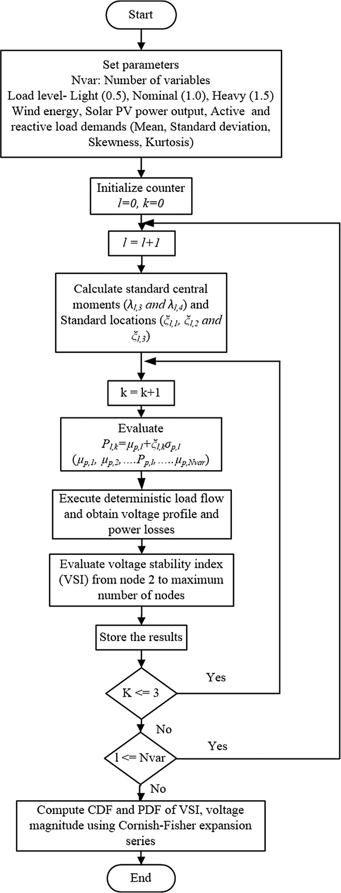
Flow chart for 2m + 1 PEM method


5 Result and Discussion
The developed probabilistic-based algorithm is examined through two test systems, i.e., IEEE 33 and 69 node radial distribution networks. The single-line diagram of 33 and 69 node radial distribution networks is shown in Figs. 5 and 6, respectively.

IEEE 33-node distribution network

IEEE 69 node radial distribution network
It is assumed that wind and solar PV-based DGs are operating at constant power mode and hence no voltage regulation is performed under normal operating conditions. For the selected radial distribution network, the substation voltage is considered at 1 pu. The selection of DG locations is limited to three, since if it is more than three, then the improvement in the percentage loss reduction is not appreciable [38]. The optimal locations of DGs for each penetration level are selected from VSI–CPF-based algorithms. In order to study the uncertainties associated with wind and solar PV-based DGs and load demand, the 2m + 1 PEM (a probabilistic power flow method) has been adopted and compared with the benchmark MCS method. The following scenarios have been investigated in this study.
Scenario I NO DG units are integrated into the distribution network (Base Case).
Scenario II Only solar PV-based DGs are integrated into the distribution network.
Scenario III Only wind energy-based DGs are integrated into the distribution network.
Scenario IV The hybrid DGs based on wind energy and solar PV are integrated into the distribution network.
All scenarios are programmed in MATLAB environment, and simulations are carried out on computer with i7 processor, 2.4 GHz with 8 GB RAM.
5.1 Test System-I (IEEE 33-Node Radial Distribution Network)
The total active and reactive power load demand in the 33-node radial distribution network is 3.72 MW and 2.3 MVAr, respectively [39]. The penetration level (PL) of DGs is incremented in steps of 10% for the particular type of renewable energy resource. The optimal locations are identified using VSI–CPF-based algorithm and shown in Table 1.
To analyze the performance, the network is simulated at three load levels, i.e., light load (0.5), nominal load (1.0) and heavy load (1.5) for each scenario. For wind energy-based DGs, the samples of wind speed are generated using Weibull PDF. The shape (a) and scale index (b) for Weibull density functions are taken as 6 m/s and 1.4, respectively. Similarly, for solar PV-based DGs, the samples of solar irradiance are generated using beta PDF. The parameters for beta density functions are α = 2.57, β = 1.6. The system load demand at any load is modeled using normal PDF, where mean (µ) is taken as the system base load with standard deviation (σ) of 5% of load demand. The random samples generated with Weibull, beta and normal PDF are mapped into corresponding PDF which are shown in Fig. 7.

a Wind speed mapped into Weibull PDF, b solar irradiance mapped into beta PDF, c active power load at node 2 mapped into normal PDF, d reactive power load at node 2 mapped into normal PDF
The various characteristics of solar PV module and wind turbine selected in this study are shown in Tables 2 and 3, respectively.
The capacity factor for a DG unit can be defined as the ratio of average output power over a period of time to its rated power output. From Figs. 8 and 9, it is observed that the wind turbine C has the highest capacity factor (0.2540), whereas the PV module B has the highest capacity factor (0.4264) and hence selected for the study.

Capacity factor for solar photovoltaic modules

Capacity factor for wind turbine modules
It is observed from Table 4, for scenario I, that power loss at light, nominal and heavy load conditions is 47.09 kW, 202.76 kW and 496.72 kW, respectively. The minimum voltage at light, nominal and heavy load is 0.9583, 0.9131 and 0.8634 pu, respectively. The minimum VSI at any node for the base case at light, nominal and heavy loads is 0.8442, 0.6969 and 0.5582, respectively.
In scenario II, the integration of solar PV-based DGs into 33-node radial distribution network is taken up. The impact on voltage stability, power losses and voltage profile of distribution network at different penetration levels (incremented from 10 to 60% in steps of 10%) of solar PV base DGs is analyzed. At the 10% penetration level, the solar PV units are placed at node 18, 33 and 32, respectively. The equal penetration level of DGs is considered at the selected optimal locations. The active power losses at 10% penetration level for light, nominal and heavy loads are 37.62, 160.19 and 386.15, respectively. Also, the minimum voltage at any node of network for light, normal and heavy load demand is improved to 0.9646, 0.9268 and 0.8859 pu, respectively. Similarly, the minimum VSI has enhanced to 0.8658, 0.7377 and 0.6161 pu for light, nominal and heavy load demands, respectively. It is also observed that the percentage improvement in voltage and VSI depends on load demand. The percentage improvement in VSI for light, nominal and heavy load is 2.5%, 5.85% and 10.72%, respectively.
Similar results are obtained for the minimum voltage of the network. Therefore, it can be concluded that under heavy load condition, DGs integration has a greater impact on the voltage profile improvement and voltage stability enhancements, whereas the percentage active power loss (% APL) reduction is independent to system load demand. At 20% solar PV-based DGs penetration, the power losses are reduced to 30.91 kW, 130.53 kW and 311.41 kW under light, nominal and heavy load demands, respectively. Approximately 15% reduction in power losses has been observed with 20% penetration level compared to 10% penetration level under all considered load demands. With the increase in penetration level (i.e., 30% and 40%) the percentage of reduction in power losses is decreasing. Under 50% penetration level, the percentage power loss reduction is almost constant compared to 40% penetration level. Above 50% penetration level, it is observed that % APL reduction is not appreciable. Therefore, the 40–50% can be considered as a penetration limit for solar PV-based DGs. Moreover, it is also observed that after 40% penetration level the percentage improvement in minimum voltage magnitude and voltage stability had also become approximately constant. In scenario III, the integration of wind energy-based DGs into 33-node radial distribution network is studied. The penetration level up to 40% is investigated in this scenario. Similar to scenario II, the wind energy-based DGs are optimally placed at nodes 18, 33 and 32, respectively. At the 10% penetration level, it is observed that the system power losses have been reduced to 39.15 kW, 167.03 kW and 405.30 kW under light, nominal and heavy load demands, respectively. Also, the minimum voltage at any node of network under light, nominal and heavy load demands has improved to 0.9646, 0.9266 and 0.8851 pu, respectively. Similarly, the minimum VSI has enhanced to 0.8659, 0.7381 and 0.6164 for light, nominal and heavy load demands, respectively. The % APL reduction under light, nominal and heavy load conditions is 16.86, 17.62 and 18.40, respectively, which are less compared to scenario II, whereas the minimum voltage and VSI improvement are almost invariant. At the 20% penetration level, the system power losses have been reduced to 36.72 kW, 156.13 kW and 375.69 kW, respectively. The minimum voltage at any node of the network under light, normal and heavy load demands has improved to 0.9703, 0.9382 and 0.9042 pu, respectively. Similarly, the minimum VSI has enhanced to 0.8874, 0.7782 and 0.6765 for light, nominal and heavy load demand, respectively. It is observed that at the 30% penetration level, the power losses have started to increase and hence 20% is considered as a suitable penetration limit for wind-based DGs.
Throughout the year, the wind speed and solar irradiance are weakly anticorrelated (−0. 4 ≤ ρ ≤ − 0. 24) [40]. To investigate the maximum penetration level of hybrid renewable-based DGs, the 70% power output from wind-based DGs and 30% power output from solar PV-based DGs have been considered. The integration of hybrid-based DGs in 33-node radial distribution network has been investigated in this scenario.
The penetration level of hybrid DGs is considered up to 40%. The nodes 18, 33 and 32 are identified for the optimal placement of hybrid energy-based DGs. Based on selected locations, three case studies are investigated. For 10% hybrid DG penetration, in case I, the solar PV-based DG is placed at node 18, whereas wind energy-based DGs are placed at nodes 33 and 32, respectively. In case II, the solar PV-based DG is placed at node 33, whereas wind energy-based DGs are placed at nodes 18 and 32, respectively. In case III, the solar PV-based DG is placed at node 32, whereas wind-based DGs are placed at nodes 18 and 33, respectively. In other words, the solar PV and wind energy-based DGs are shuffled at the three selected optimal locations at different penetration levels. It is observed from Table 5 that in case II the % APL reduction for different load demands is more compared to case I and case III. At the 10% penetration level, the % APL reduction is 20.36, 21.43 and 20.43 for light, nominal and heavy load demand, respectively. Therefore, it can be concluded that the solar PV-based DG should be placed at node 33, whereas the wind energy-based DGs should be placed at nodes 18 and 32, respectively. In case II, the power losses have been reduced to 38.50 kW, 162.29 kW and 395.23 kW, respectively. Also the minimum voltage at any node in the network has improved to 0.9648, 0.9299 and 0.8860 for light, nominal and heavy load demands, respectively. The minimum VSI in the network is also improved to 0.8664, 0.7392 and 0.6183 for light, nominal and heavy load demand, respectively.
At the 20% penetration level, similar to 10% penetration level, the % APL reduction for different load demands is more in case II as compared to cases I and III. At the 20% penetration level, the % APL reduction has increased to 28.18, 29.37 and 30.79 for light, nominal and heavy load demands, respectively. The minimum voltage at any node in the network has improved to 0.9706, 0.9392 and 0.9048 for light, nominal and heavy load demands, respectively. Also the minimum VSI in the network has been improved to 0.8882, 0.7807 and 0.6759, respectively. At the 30% penetration level only the small improvement has been observed in the % APL reduction, whereas at the 40% penetration level the % APL reduction for different load demands has started to reduce as compared to 30% penetration level. Hence, 30% penetration level is selected as a penetration limit for hybrid-based DGs in 33-node radial distribution network. Finally, the results obtained from 3PEM are compared with the MCS method in Table 6. The node voltage profile of the test system-I with solar PV, wind and hybrid DGs is shown in Figs. 10, 11 and 12, respectively. The probability density function (PDF) and cumulative distribution function (CDF) of voltage at bus 32 and VSI at various scenarios are shown in Fig. 13. Moreover, the active power losses at different load demands with solar PV, wind and hybrid DGs are shown in Fig. 14.

Node voltage profile of 33-node distribution network with solar PV DGs

Node voltage profile of 33-node distribution network with wind DGs

Node voltage profile of 33-node distribution network with hybrid DGs


PDF and CDF for voltage at node 32 and voltage stability index (VSImin) at bus 33 for various scenarios

Active power losses in 33-node network with different types of DGs penetration level
5.2 Test System-II (IEEE 69 Node Radial Distribution Network)
The total active and reactive power load demand in the 69 node radial distribution network is 3.802 MW and 2.696 MVAr, respectively. The penetration level (PL) of DGs is incremented in steps of 10% for the particular type of renewable energy resource. The optimal locations of DGs are identified using VSI–CPF-based algorithm (Table 7).
Similar to 33-node radial distribution network, the performance of 69 node radial distribution network is simulated at three load levels, i.e., light load (0.5), nominal load (1.0) and heavy load (1.5) for each scenario [41]. For wind energy-based DGs, the samples of wind speed are generated using Weibull PDF. The shape (a) and scale index (b) for Weibull density functions are taken as 6 m/s and 1.4, respectively. Similarly, for solar PV-based DGs, the samples of solar irradiance are generated using beta PDF. The parameters for beta density functions are α = 2.57, β = 1.6. The system load demand at any load is modeled using Normal PDF, where mean (µ) is taken system base load with standard deviation (σ) at 5% of load demand.
The various characteristics of solar PV module and wind turbine selected in a 69 node network are shown in Tables 2 and 3, respectively. Similar to 33-node network, owing to the high capacity factor, wind turbine C and the PV module type B are selected in this study.
It is observed from Table 8, for scenario I, that power loss of light, nominal and heavy load conditions is 51.67 kW, 255.17 kW and 561.60 kW, respectively. The minimum voltage at light, nominal and heavy load is 0.9567, 0.9092 and 0.8560 pu, respectively. The minimum VSI at any node for the base case at light, nominal and heavy load is 0.8386, 0.6851 and 0.5391, respectively.
The integration of solar PV-based DGs into 69 node radial distribution network has been investigated in scenario II. The impact on voltage stability, power losses and voltage profile of the distribution network is at different penetration levels (Incremented from 10 to 60% in steps of 10%) of solar PV base DGs have analyzed. At the 10% penetration level, the solar PV units are placed at node 61, 64 and 65, respectively. The equal penetration level of DGs is considered at the selected optimal locations.
The active power losses at 10% penetration level for light, nominal and heavy loads are 39.73, 170.83 and 415.91, respectively. Also, the minimum voltage at any node of network for light, normal and heavy load demand has improved to 0.9647, 0.9265 and 0.8847 pu, respectively. Similarly, the minimum VSI has enhanced to 0.8663, 0.7370 and 0.6131 for light, nominal and heavy load demands, respectively.
Similar to 33-node distribution network, it is observed that the percentage improvement in voltage and VSI depends upon load demand. Under heavy load condition, DGs integration has a much larger impact on the voltage profile improvement and voltage stability enhancement, whereas % APL reduction is independent to system load demand.
At 20% solar PV-based DGs penetration, the power losses are reduced to 34.41 kW, 133.11 kW and 318.93 kW under light, nominal and heavy load demand, respectively. With increase in penetration levels (i.e., 30% and 40%), the percentage of reduction in power losses is decreasing. Above 50% penetration level, it is observed that % APL reduction is decreasing. Therefore, the 50% can be considered as a penetration limit for solar PV-based DGs. It is also observed that above 50% penetration level the percentage improvement in minimum voltage magnitude and voltage stability had also become approximately constant. In scenario III, the integration of wind energy-based DGs into 69 node radial distribution network are studied. The penetration level up to 40% is investigated in this scenario. Similar to scenario II, the wind energy-based DGs are optimally placed at nodes 61, 64 and 65, respectively. At the 10% penetration level, it is observed that the system power losses have been reduced to 41.68 kW, 179.81 kW and 441.23 kW under light, nominal and heavy load demands, respectively. Also, the minimum voltage at any node of network under light, normal and heavy load demand has improved to 0.9646, 0.9262 and 0.8837 pu, respectively. Similarly, the minimum VSI has enhanced to 0.8663, 0.7377 and 0.6144 for light, nominal and heavy load demands, respectively. The % APL reduction under light, nominal and heavy load conditions is 19.33, 20.14 and 21.43, respectively, which is less compared to scenario II, whereas the minimum voltage and VSI improvement are almost invariant. At the 20% penetration level, the system power losses have been reduced to 38.51 kW, 165.05 kW and 401.68 kW, respectively. The minimum voltage at any node of network under light, normal and heavy load demands has improved to 0.9717, 0.9406 and 0.9063 pu, respectively.
Similarly, the minimum VSI has enhanced to 0.8929, 0.7883 and 0.6871 for light, nominal and heavy load demand, respectively. It is observed that at the 30% penetration level, the power losses have started to increase and hence 20% penetration level is considered as an integration limit for wind-based DGs. Similar to 33-node distribution network, to investigate the maximum penetration level of hybrid renewable-based DGs, the 70% power output from wind-based DGs and 30% power output from solar PV-based DGs have been considered. The penetration level of hybrid DGs is considered up to 40%. The nodes 65, 61 and 64 are identified for the optimal placement of hybrid energy-based DGs. Based on selected locations, three case studies are investigated. For 10% hybrid DG penetration, in case I, the solar PV-based DG is placed at node 65, whereas wind energy-based DGs are placed at node 61 and 64, respectively. In case II, the solar PV-based DG is placed at node 61, whereas wind energy-based DGs are placed at node 65 and 64, respectively. In case III, the solar PV-based DG is placed at node 64, whereas wind-based DGs are placed at node 65 and 61, respectively.
It is observed from Table 9 that for the 10% penetration level the % APL reduction in case I is higher compared to case II and case III. For case I, at 10% penetration level, the % APL reduction is 21.32, 24.14 and 23.89 for light, nominal and heavy load demands, respectively. Therefore, it can be concluded that the solar PV-based DG should be placed at node 65 whereas, the wind energy-based DGs should be placed at node 61 and 64, respectively. Also the minimum voltage at any node in the network has been improved to 0.9646, 0.9278 and 0.8837 for light, nominal and heavy load demands, respectively. The minimum VSI in the network is also improved to 0.8661, 0.7419 and 0.6130 for light, nominal and heavy load demands, respectively.
Similarly, for 20% penetration level, the % APL reduction in case I for different load demands has higher values compared to case II and case III. At the 20% penetration level, the % APL reduction has increased to 32.99, 34.62 and 36.61 for light, nominal and heavy load demands, respectively. The minimum voltage at any node in the network has improved to 0.9718, 0.9413 and 0.9081 for light, nominal and heavy load demands, respectively. Also the minimum VSI in the network has improved to 0.8925, 0.7880 and 0.6866, respectively. Similar observations are identified for 30% and 40% penetration levels. At the 40% penetration level, the % APL reduction for different load demands had started to reduce in comparison with 30% penetration level. Hence, 30% penetration level is considered to be the suitable penetration limit for hybrid-based DGs in 69 node radial distribution network. Finally, the results obtained from 3PEM are compared with the MCS method in Table 10. The node voltage profile of the test system-II with solar PV, wind and hybrid DGs is shown in Figs. 15, 16 and 17, respectively. The active power losses at different load demands with solar PV, wind and hybrid DGs are shown in Fig. 18.

Node voltage profile for 69 node radial distribution network with solar PV DGs

Node voltage profile for 69 node radial distribution network with wind DGs

Node voltage profile for 69 node radial distribution network with hybrid DGs

Active power losses in 69 node network with different types of DGs penetration level
6 Conclusions
In this paper, static voltage stability index–continuous power flow (VSI–CPF)-based method is used to identify the optimal locations of DGs in the distribution network. The different penetration levels of DGs in the radial distribution networks and their impact on total power loss, voltage profiles and voltage stability have been studied through the probabilistic approach. The IEEE 33 and 69 node radial distribution networks are utilized for validation of the proposed approach. The paper highlights the use of probabilistic-based load flow method due to uncertainties associated with solar irradiance, wind speed and load demand. The Hong’s 2m + 1 point estimation method is applied and compared with the benchmark MCS method, whereas to obtain the PDF and CDF of output random variables the Cornish–Fisher expansion series is incorporated with PEM method. Moreover, it is observed that the penetration level of DG’s in the distribution network in light of voltage stability is determined by three key factors, i.e., type of DGs, the location of DGs and load level of the network. From the simulation results, it was revealed that the maximum penetration level up to 50% is possible with solar PV-based DGs, whereas it was found 20% with wind energy-based DGs. A hybrid combination of wind and solar-based renewable DGs has penetration level up to 30%. It is also observed that the penetration level of different type of DGs in the radial distribution networks is independent of system size. Hence the authors have tried to exploit those geographical locations where wind energy is abundant, but also the solar irradiance has enough exposure. At such places instead of going only with wind-based DGs, a hybrid combination of wind and solar PV will increase the penetration level. Moreover, such locations can be easily found on wide coastal line that the tropical country like India possesses.
References
Wang, H.; Xu, X.; Yan, Z.; Yang, Z.; Feng, N.; Cui, Y.: Probabilistic static voltage stability analysis considering the correlation of wind power. In: 2016 IEEE International Conference on Probabilistic Methods Applied to Power Systems PMAPS, pp. 1–6 (2016)
Rubinstein, R.Y.: Simulation and the Monte Carlo Method. Wiley, New York (1991)
Su, C.L.: Probabilistic load flow computation using point estimate method. IEEE Trans. Power Syst. 20(4), 1843–1851 (2005)
Morales, J.M.; Perez-Ruiz, J.: Point estimate schemes to solve the probabilistic power flow. IEEE Trans. Power Syst. 22(4), 1594–1601 (2007)
Schellenberg, A.; Rosehart, W.; Aguado, J.: Cumulant probabilistic optimal power flow (P-OPF) with Gaussian and Gamma distributions. IEEE Trans. Power Syst. 20(2), 773–781 (2005)
Zhang, P.; Lee, S.T.: Probabilistic load flow computation using the method of combined Cumulants and Gram Charlier expansion. IEEE Trans. Power Syst. 19(1), 676–682 (2004)
Usaola, J.: Probabilistic load flow with wind production uncertainty using Cumulants and Cornish–Fisher expenstion. Electr. Power Energy Syst. 31(9), 474–481 (2009)
Atwa, Y.M.; El-Saadany, E.F.: Optimal allocation of ESS in distribution system with a high penetration of wind energy. IEEE Trans. Power Syst. 25(4), 1815–1822 (2010)
Ayres, H.M.; Freitas, W.; De Almeida, M.C.; Da Silva, L.C.P.: Method for determining the maximum allowable penetration level of distributed generation without steady state voltage violations. IET Gener. Transm. Distrib. 4(4), 495–508 (2010)
Hung, D.Q.; Mithulananthan, N.; Lee, K.Y.: Determining PV penetration for distribution system with time varying load models. IEEE Trans. Power Syst. 29(6), 3048–3057 (2014)
Hoke, A.; Butler, R.; Hambrick, L.; Kroposki, B.: Steady state analysis of maximum photovoltaic penetration levels on typical distribution feeders. IEEE Trans. Sustain. Energy 4(2), 350–357 (2013)
Verschueren, T.; Mets, K.; Meersman, B.; Strobbe, M.; Develder, C.; Vandevelde, L.: Assessment and mitigation of voltage violations by solar panels in a residential distribution grid. In: International Conference on Smart Grid Communications (SmartGridComm), IEEE, pp. 540–545 (2011)
Khairy, H.; El-Shimy, M.; Hashem, G.M.: Determining the maximum penetration level of solar-PV generator using eigenvalue analysis. In: 19th International Middle East Power Systems Conference (MEPCON), IEEE, pp. 293–299 (2017)
Aziz, T.; Ketjoy, N.: PV penetration limits in low voltage networks and voltage variations. IEEE Access. 5, 16784–16792 (2017)
Procopiou, A.T.; Ochoa, L.F.: Voltage control in PV rich LV networks without remote monitoring. IEEE Trans. Power Syst. 32(2), 1224–1236 (2017)
Lamberti, F.; Calderaro, V.; Galdi, V.; Piccolo, A.; Graditi, G.: Impact analysis of distributed PV and energy storage systems in unbalanced LV networks. In: IEEE Eindhoven Power Tech, Eindhoven, Netherlands, pp. 1–6 (2015)
Alam, M.J.; Muttaqi, K.M.; Sutanto D.: Distributed energy storage for mitigation of voltage-rise impact caused by rooftop solar PV. In: Power and Energy Society General Meeting, IEEE, pp. 1–8 (2012)
Liew, S.N.; Strbac, G.: Maximum penetration of wind generation in existing distribution network. IEEE Proc. Gener. Trasm. Distrib. 149(3), 256–262 (2002)
Kolenc, M.; Papic, I.; Blazic, B.: Assessment of maximum distributed generation penetration levels in low voltage network using a probabilistic approach. Int. J. Electr. Power Energy Syst. 64, 505–515 (2015)
Zio, E.; Delfanti, M.; Giorgi, L.; Olivieri, V.; Sansavini, G.: Monte Carlo simulation based probabilistic assessment of DG penetration in medium voltage distribution network. Int. J. Electr. Power Energy Syst. 64, 852–860 (2015)
Almeida, A.B.; Valenca de Lorenci, E.; Leme, R.C.; Zambroni De Souza, A.C.; Lima Lopes, B.I.; Lo, K.: Probabilistic voltage stability assessment considering renewable sources with the help of PV and QV curves. IET Renew. Power Gener. 7(5), 521–530 (2013)
Xiuhong, Z.; Kewen, W.; Ming, L.; Wanhui, Y.; Tse, C.T.: Two extended approaches for voltage stability studies of quadratic and probabilistic continuation load flow. In: International Conference on Power System Technology, pp. 1705–1709 (2002)
Haesen, E.; Bastiaensen, C.; Driesen, J.; Belmans, R.: A probabilistic formulation of load margins in power systems with stochastic generation. IEEE Trans. Power Syst. 24(2), 951–958 (2009)
Liu, K.; Sheng, W.; Hu, L.; Liu, Y.; Meng, X.; Jia, D.: Simplified probabilistic voltage stability evaluation considering variable renewable distributed generation in distribution systems. IET Gener. Transm. Distrib. 9(12), 1464–1473 (2015)
Kataoka, Y.: A probabilistic nodal loading model and worst case solutions for electric power system voltage stability assessment. IEEE Trans. Power Syst. 18(4), 1507–1514 (2003)
Hatziargyriou, N.D.; Karakatsanis, T.S.: Probabilistic load flow for assessment of voltage instability. IEE Proc. Gener. Transm. Distrib. 145(2), 196–202 (1998)
Zhang, J.F.; Tse, C.T.; Wang, W.; Chung, C.Y.: Voltage stability analysis based on probabilistic power flow and maximum entropy. IET Gener. Transm. Distrib. 4(4), 530–537 (2010)
Ran, X.; Miao, S.: Probabilistic evaluation for static voltage stability for unbalanced three phase distribution system. IET Gener. Transm. Distrib. 9(14), 2050–2059 (2015)
Ruiz Rodriguez, F.J.; Hernandez, J.C.; Jurado, F.: Probabilistic load flow for photovoltaic distributed generation using the Cornish–Fisher expansion. Electr. Power Syst. Res. 89, 129–138 (2012)
Delgado, C.; Dominguez Navarro, J.A.: Point estimate method for probabilistic load flow of an unbalanced power distribution system with correlated wind and solar sources. Int. J. Electr. Power Energy Syst. 61, 267–278 (2014)
Atwa, Y.M.; El-Saadany, E.F.; Salmu, M.M.A.; Seethapathy, R.: Optimal renewable resource mix for distribution system energy loss minimization. IEEE Trans. Power Syst. 25(1), 360–370 (2010)
Karaki, S.H.; Chedid, R.B.; Ramadan, R.: Probabilistic performance assessment of autonomous solar-wind energy conversion systems. IEEE Trans. Energy Conver. 14, 766–772 (1999)
Tian, S.; Wang, H.; Xie, X.: Probabilistic load flow analysis considering the correlation for microgrid with wind and photovoltaic system In: 5th International Conference on Electric Utility Deregulation and Restructuring and Power Technologies, pp. 2003–2008 (2015)
Fan, M.; Vittal, V.; Heydt, G.T.; Ayyanar, R.: Probabilistic power flow studies for transmission systems with photovoltaic generation using cumlants. IEEE Trans. Power Syst. 27, 2251–2261 (2012)
Modarresi, J.; Gholipour, E.; Khodabakhshian, A.: A comprehensive review of the voltage stability indices. Renew. Sustain. Energy Rev. 63, 1–12 (2016)
Chakravorty, M.; Das, D.: Voltage stability analysis of radial distribution networks. Int. J. Electr. Power Energy Syst. 23, 129–135 (2000)
Das, D.; Kothari, D.P.; Kalam, A.: Simple and efficient method for load flow solution of radial distribution netowork. Int. J. Electr. Power Energy Syst. 17(5), 335–346 (1995)
Mistry, K.D.; Roy, R.: Enhancement of loading capacity of distribution system through distributed generator placement considering techno-economic benefits with load growth. Int. J. Electr. Power Energy Syst. 54, 505–515 (2014)
Baran, M.E.; Wu, F.F.: Network reconfiguration in distribution systems for loss reduction and load balancing. IEEE Trans. Power Deliv. 4(2), 1401–1407 (1989)
Bett, P.E.; Thornton, H.E.: The climatological relationships between wind and solar energy supply in Britain. Renew. Energy 87, 96–110 (2016)
Ogunjuyigbe, A.S.O.; Ayodele, T.R.; Akinola, O.O.: Impact of distributed generators on the power loss and voltage profile of sub transmission network. J. Electr. Syst. Inf. Technol. 3, 94–107 (2016)
Author information
Authors and Affiliations
Corresponding author
Rights and permissions
About this article

Cite this article
Rawat, M.S., Vadhera, S. Probabilistic Approach to Determine Penetration of Hybrid Renewable DGs in Distribution Network Based on Voltage Stability Index. Arab J Sci Eng 45, 1473–1498 (2020). https://doi.org/10.1007/s13369-019-04023-1
Received:
Accepted:
Published:
Issue Date:
DOI: https://doi.org/10.1007/s13369-019-04023-1