Structural health status assessment of a cable-stayed bridge by means of experimental vibration analysis

Abstract

The results of an experimental dynamic analysis and structural modelling of the Indiano Cable-Stayed Bridge in Florence, Italy, are presented in this paper. Ambient and traffic-induced vibration tests were first carried out. These allowed extracting the dynamic characteristics of the structure in terms of resonance frequencies, modal shapes and damping. The experimental results were used to set up a finite element model. The geometrical characteristics and the mechanical properties of the materials used in the structural design of the bridge were assumed. The model was then used to evaluate the effects of the static and seismic loads according to the present Italian Technical Code. The results pointed out the good performance of the bridge, even though it had been designed without accounting for the seismic actions.

1 Introduction

Italy, but also other countries in the world, has a large patrimony of bridges. These are masonry arch bridges, concrete bridges and steel bridges of over 50 years. Most of them were built when technical codes were quite different from the present codes. Therefore, they were designed by using travelling loads different from the present ones. The preservation of these structures is an important issue to guarantee their efficiency, durability and reliability. This can be pursued by means of the definition of a proper maintenance programme to avoid worse and non-reversible damage due to lack of maintenance.

Probably thanks to a conservative design procedure and reserves of strength, several bridges are still operational on today’s road and railway networks. For these, the goal should be the reduction in the maintenance costs and the increase in the safety level. In other cases, a retrofit is needed to adequate the structure to the present loads, such as the seismic actions according to the new seismic hazard knowledge.

The classic maintenance on request, which implies a retrofitting intervention only if damage is already occurred, should be avoided. Alternatively, a cyclic preventive maintenance should be done, which aims at preventing any damage and is based on a life cycle assessment of the structure and its component to define the optimum maintenance period.

Actually, a suitable preventive maintenance should be based on the experimental evaluation of the effective structural health status. This can be done by means of a continuous monitoring, in which the health status of the bridge and its components is continuously checked, or, alternatively, by means of periodic tests on the structure and materials. Obviously, any intervention should be made on the basis of the effective level of damage.

With reference to the adequacy against the seismic actions, the experimental vibration analysis assumes a fundamental role. This allows to find out the dynamic characteristics of a structure and to assess its possible dynamic behaviour during seismic events. On the other hand, the experimental vibration analysis allows to gain experience on the dynamic behaviour of bridges, in general, useful for the future design and analyses.

With particular reference to cable-stayed bridges, several examples of previous experimental vibration analysis can be found in the literature. Whenever possible, low-amplitude tests are used to verify the results of analytical studies. Relevant examples of dynamic testing were already carried out on bridges some decades ago. Among the most interesting experiences, it is worth reminding the studies on the Adamillo Cable-Stayed Bridge in Sevilla [1], the Pedestrian Bridge in Burlington, Vermont [2], the Tampico Bridge in Mexico [3] and the Garigliano Cable-Stayed Bridge in Italy [4]. The vibrations due to road roughness were analysed by Wang and Huang [5]. Dynamic identifications of cable-stayed bridges for seismic analysis purposes were reported in [6, 7].

More recently, the operational modal analysis (OMA) using different identification techniques for a cable-stayed bridge was proposed by Benedettini and Gentile [8], together with the finite element modelling and tuning. Magalhães et al. [9] presented the ambient and free vibration analyses of one of the most interesting bridges of the last decades, the Millau Viaduct, and highlighted the importance of modal identification at commissioning stage and comparison with models used in the design. The Sutong Cable-Stayed Bridge, which is the second longest cable-stayed bridge in the world, was investigated by Mao et al. [10] in the framework of long-term monitoring, showing variability of the properties associated with traffic and temperature. For the longest cable-stayed bridge, the Russky Bridge in Vladivostok, Syrkov and Krutikov [11] performed a risk analysis based on a design 80-year life cycle, which allowed designing a suitable monitoring system of the structure. The life duration was based on the estimates of cable system durability. A state of the art of Structural Health Monitoring (SHM) of cable-stayed bridges is presented in [12].

The Indiano Cable-Stayed Bridge in Florence, Italy, is the subject of this paper. It was designed in the 1970s of the last century, when the site of the bridge was not classified as seismic area. Therefore, the structural design did not account for the seismic actions. It was opened to the traffic in 1977. The bridge was tested by recording ambient and traffic-induced vibrations, on the basis of which a finite element model was set up. This allowed a check of the bridges under the present static and dynamic loads according to the present Italian Technical Code.

After the experimental analysis, the bridge was retrofitted. This intervention interested the girder bearings and did not change the global dynamic characteristics of the structure. Therefore, the results obtained can be considered still valid for a static and seismic check of the bridge.

2 The Indiano Cable-Stayed Bridge

A general view of the Indiano Cable-Stayed Bridge, over the Arno River in Florence, is shown in Fig. 1. The longitudinal section and the plan view with the general dimensions of the bridge are shown in Fig. 2.

Fig. 1

The Indiano Cable-Stayed Bridge, Florence, Italy

Fig. 2

General dimensions of the bridge and sensor layout

The main span is 189.1 m long. It is suspended by two fans, each one composed of three couples of stays, radiating from the tops of the two steel towers (Fig. 3), and is supported at its ends by two piers by means of sliding supports. The piers are structurally independent of the other parts of the cable-stayed bridge.

Fig. 3

Cables fanning from one of the steel pylons (view from the walkway)

Cables are longitudinally regularly spread of 30.5 m along the deck, but the longitudinal distance between the anchorages of the central cables is only 6.1 m. The stays of each pair are 3.0 m spaced from the centre line of the girder; therefore, their contribution to the global torsional stiffness is very low. Two earth anchored back stays start from the top of each tower and are constrained to an external gravity anchoring, 65.5 m from the pylon bases. Each stay is composed of three cables (Fig. 4).

Fig. 4

One of the anchor stays, composed of two sets of three cables, with its external anchorage

The pylons have steel box cross section and a height of about 55.0 m from the ground. They are fully constrained at their foundations, which are founded on large piles, and linked to the foundation of the anchor stays by means of a pre-stressed concrete truss, which is supposed to support the horizontal component of the tower reaction force.

With reference to the cross section, the main span can be divided into three portions. In the central one (zone M in Fig. 2), whose length is 128.1 m, two boxes spaced of 6.0 m compose the cross section (Fig. 5). They are linked to one another, at the upper and lower levels, by means of truss structures. The boxes have a width of 4.0 m and a height varying from 2.6 to 1.6 m. Cantilever beams start from the boxes to support the external portion of the road. In the two zones near the ends (zones L and R in Fig. 2), the cross section becomes a three-box cross section. In both cases, the beam has a high torsional stiffness.

Fig. 5

Cross section of the girder

A walkway for pedestrians and bicyclists is suspended to the girder (Fig. 6). Due to its very high deformability, its contribution in the dynamic behaviour of the bridge is negligible.

Fig. 6

The walkway for pedestrians and bicyclists suspended to the girder

Parallel wires (∅7) stay cables with steel tensile strength of 1700 MPa were used, whereas the tensile strength of the steel plates used for girder and tower boxes was 520 MPa. Finally, 420 MPa strength steel was adopted for ribs and trusses.

The bridge was designed according to the technical code of the construction time.

3 Experimental vibration analysis

The experimental vibration analysis was carried out by using seismometers connected to an acquisition system. These were deployed in different configurations in order to analyse the vertical, longitudinal and transversal vibrations. The acquisition system allowed also analysing the recordings in real time, so it was possible to perform a preliminary analysis of the experimental data during the experimental phase. The experimental analysis allowed to find out the vibration amplitudes under traffic loads and to get the dynamic characteristics of the bridge.

Seismometers were deployed as follows (Fig. 2):

• Two sensors were at the base of the right tower (NE tower), in the longitudinal (S_0L) and transversal direction (S_0T), respectively,

• one sensor was deployed at the top of the left tower (SW tower) in the longitudinal direction (T_1L),

• two sensors were at the top of the right tower, in the longitudinal (T_2L) and transversal direction (T_2T), respectively,

• other sensors were deployed on the girder in the vertical, transversal or longitudinal directions. They were positioned eccentrically with respect to the longitudinal axis. In detail, they were deployed at the middle (D₀ and D′₀), at the left (SW) end of the girder central portion (D₁) and at the right (NE) end of the girder central portion (D₂ and D′₂).

Several time histories lasting 64 s were recorded for each configuration to show repeatability of the vibrational characteristics and to get average values of the characteristics.

During the test, the temperature was about 10 °C with very low variability around this value. The maximum wind speed was of only 20 km/h. Due to the low values of the speed, its influence on the structural behaviour was scarce.

3.1 Frequency domain analysis

The recorded data were analysed in the frequency domain, by plotting the power spectral densities (PSDs) of all the records and cross-spectral densities (CSDs) for all the significant couples of locations. The following resonance frequencies were found, associated with the described deformed shapes, which will be compared with those obtained from the mathematical model.

• Peaks at 0.61 Hz are clearly identifiable in the spectra of the records obtained at the top of the towers in the longitudinal direction (Fig. 7, T_1L and T_2L) and in those of the deck in the vertical direction (Fig. 8, D_1V and D_0V). From the CSDs, one can see that the records at the top of the towers in the longitudinal direction (T_1L and T_2L) are 180° out of phase (Fig. 9) and all the records at the deck in the vertical direction (D_1V, D_0V and D_2V) are in phase (Fig. 10). Furthermore, the record at the top of tower 2 in the longitudinal direction and that at the mid-span of the deck in the vertical direction (T_2L and D_0V, respectively) are in phase (Fig. 11). Therefore, the associated modal shape is symmetric around the mid-span, and when the towers move outwards, the deck moves upwards (see Fig. 23, mode 1). It is worth reminding that the same resonance frequency was estimated at the end of construction by a free vibration test. The bridge was excited by dropping a suspended mass of 800 kNs²/m from the middle of the span [13].

  Fig. 7

  

  PSDs of records at the top of the towers in the longitudinal direction

  Fig. 8

  

  PSDs of records at the deck in the vertical direction

  Fig. 9

  

  CSDs of records in the longitudinal direction at the top of the towers

  Fig. 10

  

  CSDs of records in the vertical direction of the deck

  Fig. 11

  

  CSDs of records in the longitudinal direction at the top of the tower 1 and in the vertical direction in the mid-span of the deck

• The spectrum of records at the deck in the longitudinal direction (D′_0L) shows a very apparent peak at 0.81 Hz. This frequency is present also in the spectra of the records at the top of the towers, as demonstrated by the cross-spectrum T_2L–D_0L (Fig. 12). As a result, the modal shape associated with this frequency consists in the longitudinal movement of tower and deck (see Fig. 23, mode 2).

  Fig. 12

  

  CSDs of records at the top of the tower 2 and the mid-span of the deck in the longitudinal direction

• Peaks at frequency 0.87 Hz can be identified in the spectra of the deck records in the transversal direction (D_1T, D_0T and D_2T, Fig. 13). These are in phase (Fig. 14) and the corresponding modal shape (see Fig. 23, mode 3) is the first mode in the transversal direction of the girder. The towers do not contribute to this mode.

  Fig. 13

  

  PSDs of records at the deck in the transversal direction

  Fig. 14

  

  CSDs of records of the deck in the transversal direction

• Peaks at frequencies 1.04 and 1.15 Hz are apparent in the spectra of records in the transversal direction at the top of the tower 2 (Fig. 15, T_2T). The deck does not contribute to these modes (see Fig. 23, modes 4 and 5). Records of sensors D_0V and D′_0V are 180° out of phase at 1.15 Hz.

  Fig. 15

  

  PSD of record at the top of the tower 2 in the transversal direction

• The spectra of the records in the longitudinal direction at the top of the towers show peaks at 1.41 Hz (Fig. 7, T_1L and T_2L). The signals are in phase at this frequency (Fig. 9). Low peaks are also visible in the spectra of the vertical records at the girder (Fig. 8).

• At frequency 1.61 Hz, T_1L and T_2L are 180° out of phase (Fig. 9); therefore, the towers move anti-symmetrically around the mid-span. D_1V and D_2V are in phase at this frequency, while D_0V and D_2V are 180° out of phase. As a result, the girder shaped symmetrically with three half waves (see Fig. 23, mode 7).

• At frequency 2.25 Hz, T_1L and T_2L are in phase (Fig. 9) and D_1V and D_2V 180° out of phase (Fig. 10). A two-wave modal shape is associated with this frequency. In this case also, the towers take part in the mode (see Fig. 23, mode 8).

• The second transversal mode of the girder is associated with the frequency 2.61 Hz, as pointed out by the sensors in the transversal direction on the deck (Fig. 13) (see Fig. 23, mode 9).

In Table 1, the resonance frequencies individualized for each sensor location are listed. The equivalent viscous damping ratios, estimated by using the half power bandwidth method, are also summarized in Table 3. The values of damping obtained were quite high in comparison with the usual ones for cable-stayed bridges. This was attributed to the presence of several sources of damping in joints and bearings at the time of the experimental campaign. It is restated herein that damping due to sliding supports increases for oscillation with very small amplitude [14].

Table 1 Experimental resonance frequencies and estimated damping

3.2 Time domain analysis

The recorded velocities were then integrated in the frequency domain to get corrected displacement time histories.

In Fig. 16, the displacement time histories recorded at the mid-span of the deck, in the transversal and longitudinal direction, respectively, are plotted. The corresponding particle motion is plotted in Fig. 17 together with the angle distribution. As one can see, the motion occurs in the transversal direction, preferentially. Anyway, the displacements in the longitudinal direction are of the same order. This is certainly one of the characteristics of the dynamic behaviour of the Indiano Bridge, i.e., the presence of high-amplitude longitudinal vibrations. The absence of longitudinal restraints is usual in cable-stayed bridges, but in this case the above occurrence is amplified because of the absence of the side cable-stayed spans and because the system is not self-anchored.

Fig. 16

Contemporary displacement time histories at the deck mid-span in the a transversal and b longitudinal direction

Fig. 17

a Particle motion (mm) and b angle distribution at the mid-span of the deck

Analogously, in Fig. 18 the displacement time histories recorded at the top of the NE tower are plotted, in the transversal and longitudinal direction, respectively, and the corresponding particle motion is plotted in Fig. 19 together with the angle distribution. In this case also, the motion in the transversal direction is higher than in the longitudinal direction.

Fig. 18

Contemporary displacement time histories at the top of the right (NE) tower

Fig. 19

a Particle motion (mm) and b angle distribution at the top of the right (NE) tower

3.3 Free-field noise measurements

Free-field noise measurements were carried out around the bridge to assess possible effect of the site conditions on the dynamic response of the bridge. Three seismometers were kept at the basement of the right tower in the longitudinal, transversal and vertical direction (S_0L, S_0T, S_0V). Three other sensors, arranged in the same directions, were deployed, in different times, at three different positions, about 50 (S_1L, S_1T, S_1V), 100 (S_2L, S_2T, S_2V) and 200 m (S_3L, S_3T, S_3V) away from the right tower of the bridge, in a direction perpendicular to the longitudinal direction of the bridge.

For each configuration, several tests lasting 64 s were carried out. Recorded data were analysed in the frequency domain. Some of the natural frequencies of the bridge appear in the PSD ratios between the horizontal and vertical component [15] at each position, for a few records. This was probably due to the different excitation level from the bridge traffic.

The analysis pointed out the presence of two peaks at frequencies below 0.5 Hz in the horizontal to vertical component spectral ratios as well as in the ratios between the PSDs of the same components at different positions. These are common values for alluvium soil. Therefore, there is not relationship between the behaviour of the soil and the natural frequencies of the bridge.

4 Finite element model

A finite element model of the bridge was developed using MIDAS GEN © code (Fig. 20). The geometrical and mechanical characteristics of the bridge were deduced from the structural design drawings obtained via the Technical Office of the City Hall in Florence [16].

Fig. 20

Finite element model of the bridge

The towers have been considered fully constrained at their basements. The girder has been considered simply supported at its ends, where longitudinal displacements are allowed but not the transversal and vertical displacements nor torsional rotations.

The girder and the pylons have been modelled by using steel beam elements, with a Young’s modulus E = 210,000 MPa. Rigid limbs have been offset from both the girder and the towers, in order to accommodate correctly the cable attachments. The bending and torsional stiffness of the girder are variable along the span. Therefore, the girder has been divided into three portions; in each of them, the geometrical characteristics have been assumed to be constant and equal to the average values.

The geometrical characteristics of the towers change along their axis. The geometrical characteristics, used to develop the mathematical model, are listed in Table 2 for the deck and in Table 3 for the pylons in which:

Table 2 Geometrical properties and Young’s modulus of the girder beam elements

Table 3 Geometrical properties and Young’s modulus of the tower beam elements

• A is the cross-sectional area,

• I_x and I_y are the second moments, relative to the transversal axes of the cross section in the local reference systems (z is the longitudinal axis in both local systems),

• J is the torsion factor.

Cables have been modelled as truss elements. The reduction in their axial stiffness due to the sag has been accounted for assuming equivalent reduced Young’s modules [17, 18]. If $\sigma$ is the stress under dead loads and $\Delta \sigma$ the increment in stress due to travelling loads, the tension parameter can be defined as:

$$k = 1 + \frac{\Delta \sigma }{\sigma }$$

and the secant equivalent modulus in the stress path from $\sigma$ to $\sigma + \Delta \sigma$ is:

$$E_{\text{s}}^{*} = \frac{E}{{1 + \varphi^{2} \left( {\frac{1}{24} + \frac{E}{\sigma } \cdot \frac{k + 1}{{\varphi^{2} + 24k^{2} }}} \right)}}$$

where $\varphi = {{\gamma \lambda } \mathord{\left/ {\vphantom {{\gamma \lambda } \sigma }} \right. \kern-0pt} \sigma }$ is a cable shape parameter in which $\gamma$ and $\lambda$ are the weight per unit volume and the cable span, respectively. Putting $k = 1$, we deduce the tangent modulus $E_{t}^{*}$ under dead loads. In Table 4, the cross-sectional areas and the defined tangent modules of the cables are provided.

Table 4 Cross-sectional areas and apparent moduli of the cables

4.1 Modal analysis

The mass of the girder (= 140 kNs²/m²) has been increased by 10% to account for the vehicles and additional masses, which were present during the tests. The resulting distributed mass of 154 kNs²/m² and the mass inertia around z-axis of 4020 kNs²/m have been lumped at the girder nodes. The increment in loads being very low, the tangent modules $E_{t}^{*}$ have been considered for the cables.

The modal analysis resulted in the resonance frequencies listed in Table 5. The corresponding first nine modal shapes are plotted in Fig. 21. The modal shapes of the numerical model and the corresponding frequencies are quite similar to the experimental ones. Discrepancies have been found only in the first resonance frequencies corresponding to the transversal and longitudinal motions of the deck. These discrepancies can be endorsed to a non-exact estimation of the distribution of the stiffness and masses. Furthermore, the numerical model pointed out other resonance frequencies. These would be associated with torsional movements of the deck, but were not excited during the tests.

Table 5 Frequencies of the numerical model and experimental resonance

Fig. 21

Modal shapes

5 The effects of permanent and live static loads

The static analysis was carried out. First, the effects of the structural self-weight W₁ and the other permanent loads W₂ were calculated. Then, the following live load conditions were considered, in accordance with the Italian Technical Code [19]:

• C1. One or more lanes, 3 m wide, each of which includes two concentrated loads Q_ik and a distributed load q_ik (Fig. 22), deployed in order to maximize the effects in the girder, according to the following rules:

  • Lane 1 with Q_1k = 300 kN and q_1k = 9.00 kN/m².

  • Lane 2 with Q_2k = 200 kN and q_2k = 2.50 kN/m².

  • Lane 3 with Q_3k = 100 kN and q_3k = 2.50 kN/m².

  • Lane 4 with only q_4k = 2.50 kN/m².

  Fig. 22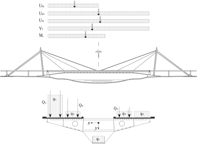

  

  Longitudinal and transversal load distributions

  The remaining areas, as well as the pedestrian suspended walkway, were loaded with q_rk = 2.50 kN/m². In practice, the two cases of lanes 1 and 2 and lanes 1 to 4 were considered.

  The positions of Q_1k and q_1k vary according to the influence line of the characteristic to maximize. In Fig. 22, the load conditions that maximize the most important displacement components and internal forces are shown. These are the vertical, longitudinal and transversal displacements of the girder (U_DV, U_DL and U_DT, respectively), the longitudinal displacement of the towers (U_TL), the axial force in the tower (V_T) and the bending moment M_x in the girder.

• C2. A longitudinal load, which simulates a braking column of vehicles, whose resultant is equal to $q_{3} = 0.6 \cdot 2Q_{1k} + 0.10 \cdot q_{1k} w_{1} L$ (with q_1k = 9.00 kN/m², w₁ = 3.00 m, L is the length of the travelling load q_1k and 180 ≤ q₃ ≤ 900 kN). This load is assumed uniformly distributed along the loaded length L.

• C3. A transversal wind load q₅ = 1.63 kN/m², which corresponds to a mean wind speed of about 100 km/h, acting on the entire span of the bridge in the presence of a vehicle column of 3.00 m height. Obviously a correct analysis of wind action would require a more detailed study to account for the dynamic effects. The maximum transversal displacement of the girder (U_DT) and the maximum bending moment M_y in the girder are expected from this load condition.

The effects, in terms of stresses and displacements in selected elements and sections, due to all these static loads, acting separately with their defined characteristic values, were calculated. In this case, the secant elastic modules for the cables, previously defined and evaluated for each load condition, were used. The results are reported in Table 6 together with the corresponding values under permanent loads.

Table 6 Maximum displacement components and internal forces due to the characteristic values of the permanent and service live loads (displacements and torsion rotation θ_D of the deck are evaluated at the mid-span section, torsion moment at the end section)

6 Seismic analysis

The results of the static analysis were compared with the effects due to the seismic actions. According to the Italian Technical Code, the seismic hazard is described by means of the elastic response spectra at the site, defined for three values of the exceedance probability in 50 years, P_NCR,50. The minimum value P_NCR,50 = 2% is obviously related to our knowledge about the historical seismicity.

The spectra are defined by means of three parameters:

• The horizontal maximum acceleration a_g on rigid soil (type A),

• the structural amplification factor F₀, which is the ratio between the maximum value and the value at T = 0,

• the value of the period $T_{C}^{*}$ corresponding to the end of the maximum constant acceleration range.

For the site of the Indiano Bridge, these are plotted in Fig. 23 versus P_NCR,50. The seismic local amplification is accounted for a soil amplification factor S, which is a function of the soil characteristics and of the acceleration. The soil can be assimilated to a soil type C. The corresponding elastic spectra for significant values of P_NCR,50 are plotted in Fig. 24.

Fig. 23

Hazard parameters for the Indiano Bridge site

Fig. 24

Horizontal and vertical elastic response spectra at the Indiano Bridge site

Seismic response spectrum analyses were carried out, in which the three following combinations of the three components of the seismic action were considered (L = longitudinal, T = transversal, V = vertical):

$$\begin{aligned} &E_{\text{L}} + 0.3 \cdot E_{\text{T}} + 0.3 \cdot E_{\text{V}} \quad 0.3 \cdot E_{\text{L}} + E_{\text{T}} + 0.3 \cdot E_{\text{V}} \quad \\&0.3 \cdot E_{\text{L}} + 0.3 \cdot E_{\text{T}} + E_{\text{V}} \end{aligned}$$

For each combination, the effects of the vibration modes have been added according to the complete quadratic combination (CQC) rule. The results obtained for the three values of P_NRC,50 are reported in Table 7.

Table 7 Effects of the seismic action for different P_NRC (displacements and torsion rotation θ_D of the deck are evaluated at the mid-span section, torsion moment at the end section)

6.1 Comparison between the static and seismic load conditions

The comparison between Tables 6 and 7 points out the following considerations.

With reference to the static analysis, the load conditions C1 give the maximum values for the vertical (U_DV) and longitudinal displacements (U_DL and U_TL) and also for the bending moment M_xand the torsion moment M_z in the girded, the axial force in the towers (V_T) and the forces in all the stays (S₀, S₁, S₂, S₃). The longitudinal displacement due to load condition C2 is lower than that of load condition C1. The load condition C3, related to the wind action, gives the maximum values for the transversal displacements (U_DT and U_TT) and the bending moment M_y.

Considering the seismic action with P_NRC,50 = 10%, the transversal displacements of the deck and the tower (U_DT and U_TT, respectively) and the bending moment M_y in the deck are higher than those due to the wind loading. For higher value of P_NRC,50, also the longitudinal displacement of the deck U_DL becomes more severe than that due to static loads.

With reference to the cables, the major axial forces are induced by the seismic combination in which the vertical seismic action is prevalent. Anyway, the stresses under seismic actions are always lower than those due to travelling loads (load C1). The maximum value due to seismic actions occurs in cable S1, in which for the exceedance probability of 2% the force is about 35% of the forces under permanent loads.

It is worth reminding that the effects of the seismic actions reported in Table 7 were calculated with reference to the elastic spectra, i.e., assuming a behaviour factor unitary for the bridge. This is certainly on the safe side but could be justified by the generally low ductility of the cables and also by the presence of structural elements subject to compression axial forces, such as the towers. Instead, the effects due to the static loads were evaluated with reference to the service loads (characteristic values). They should be amplified by means of the partial load factors (usually varying up to 1.5) to get the corresponding values at the ultimate limit state.

Furthermore, the seismic check of a bridge is usually carried out in the absence of other variable loads. Therefore, on the basis of the values shown in Tables 6 and 7 and of these latest considerations, one can state that the total internal forces in the presence of seismic actions with exceedance probability of 2% are lower than those in the presence of the other variable loads, except for the bending moment M_y, which is much higher than that due to the wind.

7 Conclusions

The Indiano Cable-Stayed Bridge, which was designed when Florence was not classified as seismic area, has been studied by means of experimental vibration analysis. The recordings have been analysed both in time and frequency domain. The dynamic characteristics of the structure and the effects of the ambient and traffic-induced vibrations have been pointed out. The results have been also used to set up a finite element model of the bridge. This has been used to analyse the structural behaviour under static and seismic loadings according to the present Italian Technical Code.

The results can be summarized as follows:

• Several resonance frequencies are clearly identified from the observed dynamic response data and also from modal analyses using a mathematical model. The modal shapes inferred from observed data are very similar to those obtained from modal analyses using the mathematical model. The differences can be attributed to the presence of different masses during the tests.

• Traffic-induced vibration amplitudes, both in vertical and in longitudinal directions, are very high, so that to determine frequent needs of maintenance works, the structure shows relevant displacements also in the longitudinal direction, due to motion of the towers.

• Values of estimated structural damping are very high compared with those determined for cable bridges. This occurrence is related to the presence of several sources of damping (friction) in joints and in bearings.

• The comparison between the effects of the seismic actions and those of the static loads pointed out in general the good performance of the bridge, with a major effect of seismic action related to the lateral deflection of the deck, which is much more relevant with respect to static wind.

References

Casas JR (1995) Full-scale dynamic testing of the Adamillo cable-stayed bridge in Sevilla (Spain). Earthq Eng Struct Dyn 24(1):35–51. https://doi.org/10.1002/eqe.4290240104
Gardner-Morse MG, Huston DR (1993) Modal identification of cable-stayed pedestrian bridge. J Struct Eng 119(11):3384–3404. https://doi.org/10.1061/(ASCE)0733-9445(1993)119%3A11(3384)
Murià-Vila D, Gomez R, King C (1991) Dynamic structural properties of cable-stayed Tampico bridge. J Struct Eng 117(11):3396–3416. https://doi.org/10.1061/(ASCE)0733-9445(1991)117%3A11(3396)
Clemente P, Marulo S, Lecce L, Bifulco A (1998) Experimental modal analysis of the Garigliano cable-stayed bridge. Soil Dyn Earthq Eng 17(7–8):485–493. https://doi.org/10.1016/S0267-7261(98)00022-0
Wang TL, Huang D (1992) Cable-stayed bridge vibration due to road surface roughness. J Struct Eng 118(5):1354–1374. https://doi.org/10.1061/(ASCE)0733-9445(1992)118%3A5(1354)
Hao Q, Jufeng S, Pingming H (2017) Study on dynamic characteristics and seismic response of the extradosed cable-stayed bridge with single pylon and single cable plane. J Civil Struct Health Monit 7:589. https://doi.org/10.1007/s13349-017-0243-6
Elkady AZ, Seleemah MA, Ansari F (2018) Structural response of a cable-stayed bridge subjected to lateral seismic excitations. J Civil Struct Health Monit 8:417. https://doi.org/10.1007/s13349-018-0282-7
Benedettini F, Gentile C (2011) Operational modal testing and FE model tuning of a cable-stayed bridge. Eng Struct 33(6):2063–2073. https://doi.org/10.1016/j.engstruct.2011.02.046
Magalhães F, Caetano E, Cunha A, Flamand O, Grillaud G (2012) Ambient and free vibration tests of the Millau Viaduct: evaluation of alternative processing strategies. Eng Struct 45:372–384. https://doi.org/10.1016/j.engstruct.2012.06.038
Mao JX, Wang H, Feng DM, Tao TY, Zheng WZ (2018) Investigation of dynamic properties of long-span cable-stayed bridges based on one-year monitoring data under normal operating condition. Struct Control Health Monit 25(5):1–19. https://doi.org/10.1002/stc.2146
Syrkov AV, Krutikov OV (2014) Lifecycle optimization for Vladivostok-Russky isle bridge by means of risk analysis and monitoring. Autom Remote Control 75(12):2217–2224. https://doi.org/10.1134/S000511791412011X
Li H, Ou J (2016) The state of the art in structural health monitoring of cable-stayed bridges. J Civil Struct Health Monit 6:43–67. https://doi.org/10.1007/s13349-015-0115-x
Augusti G, Chiarugi A, Vignoli A (1979) Analisi sperimentale di un ponte strallato. In: Proc. of the 7th Italian conference on steel structures (Torino 1979), C.T.A. Milano (in Italian)
Kawashima K, Unjoh S, Tunomoto M (1993) Estimation of damping ratio of cable-stayed bridges for seismic design. J Struct Eng 119(4):1015–1031. https://doi.org/10.1061/(asce)0733-9445(1993)119%3a4(1015)
Nakamura Y (1989) A method for dynamic characteristics estimation of subsurface using microtremor on the ground surface. QR RTRI 30(1):25–33
Clemente P, Celebi M, Bongiovanni G, Rinaldis D (2004) Seismic analysis of the Indiano cable-stayed bridge. In: Proc. of the 13th world conference on earthquake engineering (13WCEE, Vancouver, 1–6 August), Paper No 3296, IAEE & CAEE, Mira Digital Publishing, Saint Louis
Clemente P, D’Apuzzo M. Analisi del modello generalizzato di ponte strallato” Fondazione Politecnica per il Mezzogiorno d”Italia, Giannini Napoli, 1990, No 162 (in Italian)
D’Apuzzo M, Clemente P (1990) Progetto preliminare dei ponti strallati. Autostrade Autostrade-Italstat Roma 3:70–78 (in Italian)
NTC-2018 (2018) Norme tecniche per le costruzioni, DM MIT 17.01.2018, Supplemento ordinario alla Gazzetta Ufficiale n. 42 of February 20, 2018 - Serie generale
Author information
Authors and Affiliations
Corresponding author
Additional information
Publisher's Note
Springer Nature remains neutral with regard to jurisdictional claims in published maps and institutional affiliations.
Rights and permissions
About this article
Cite this article
Clemente, P., Bongiovanni, G., Buffarini, G. et al. Structural health status assessment of a cable-stayed bridge by means of experimental vibration analysis. J Civil Struct Health Monit 9, 655–669 (2019). https://doi.org/10.1007/s13349-019-00359-2
Received:
Accepted:
Published:
Issue Date:
DOI: https://doi.org/10.1007/s13349-019-00359-2