An optimal learning-based controller derived from Hamiltonian function combined with a cellular searching strategy for automotive coldstart emissions

Abstract

The main objective of this study is to propose a novel algorithmic framework for the implementation of a nonlinear controller for reducing the amount of tailpipe hydrocarbon emissions in automotive engines over the coldstart period. To this aim, the control problem for a given engine is formulated in the form of the standard Bolza problem, and then, the concepts of Euler–Lagrange equation and Hamiltonian function are taken into account to calculate the optimal states, co-states, and control input signals. An extreme learning machine is also linked to an experimentally validated nonlinear state-space representation of the engine during the coldstart to approximate the values of exhaust gas temperature and engine-out hydrocarbon emissions, which are two key variables for the considered control problem. To solve the resulting system of equations, a cellular variant of the particle swarm optimization technique is implemented and the existing nonlinear system of equations is solved heuristically. In addition, some constraints are exerted on the control signals to guarantee the smooth operation of the engine by applying the calculated controlling commands. Finally, the authenticity of the resulting optimal controller is validated against a classical Pontryagin’s minimum principle-based control system. Generally, the findings demonstrate the effectiveness of the proposed control methodology to reduce coldstart hydrocarbon emissions in automotive engines.

1 Introduction

Over the past decades, an astonishing trend has emerged towards developing effective controllers to improve the performance of vehicles [1]. The main reason for this phenomenon lies in the fact that enhancing the performance of automobiles by means of designing and implementing more advanced controllers is much more cost-effective compared to devising and applying new hardware for them. In particular, it has been demonstrated that applying optimal controlling algorithms can significantly decrease the fuel consumption and emissions of vehicle systems without any additional costs for replacing or modifying any other part of the vehicle. In this way, a proper controller can be designed to improve different aspects of automotive engines as one of the most important components of the vehicle. For improving the performance of a given engine, several operating metrics can be defined which focus on advancing specific characteristics of the engine, and thus, certain controllers with pre-defined goals can be designed to enhance each of those features. To use a new controller for improving the vehicle’s engine performance, it is only required to implement the new control algorithm (written in a certain programming environment) on the related electronic control unit (ECU) and apply it to regulate the engine functioning during a driving cycle [2].

After lots of experiments and analyses by automotive engineers and researchers, nowadays, there is a wide consensus on the above-mentioned claim about vehicle control systems, and there has been an increasing interest among the automotive research community to come up with advanced controlling strategies to be used at the hearts of vehicle systems’ ECUs to enhance their performance [3]. By investigating the archived literature on designing controllers for automobiles, it can be inferred that the main focus of these studies has been on developing control systems for reducing the amount of emissions [4], decreasing fuel consumptions [5], decreasing travel times [6], and increasing the safety of vehicle motions [7] during the driving period. Various types of offline, online, model-based, and heuristic controllers have been designed so far to comply with the above-mentioned objectives. Among the existing controllers, those implemented based on the concept of Pontryagin’s minimum principle (PMP) [8], model predictive control (MPC) [9], fuzzy theory [10], linear quadratic tracking system (LQTS) [11], sliding mode control (SMC) [12], neural controlling systems [13], switching hybrid control system (SHCS) [14], game theoretic-based controllers [15], robust state feedback stabilization controller [16], and dynamic programming (DP) [17] have been proven to show the most promising results. However, the research on designing more advanced vehicle controllers is still an open area of investigation, and researchers are trying very hard to take advantage from advanced mathematics-based and computational intelligence-based tools to increase the effectiveness of the current controllers [18].

Arguably, among the above-mentioned objectives, reducing the emission rate of vehicles stands in the first place. This is because of the existing tight governmental regulations concerning the environmental issues and global warming phenomenon, which have enforced industrialists to put a considerable amount of financial and technological forces on improving the performance of their products. In line with such a concern, environmental agencies and governmental authorities have exerted some provisions which oblige the automotive industry to move towards designing green vehicle technologies which emit a very trivial amount of pollutants [19]. Although the ultimate goal of the automotive industry is to replace the current gasoline-powered vehicles with electrified vehicles, this choice seems not to be feasible at the moment as there are still some technical problems for the widespread use of them. Furthermore, the initial investigations indicate that, by the current battery technologies, the production of fully electric vehicles is not an economical choice for both industrialists and consumers, and the final price as well as maintenance cost of electric drive vehicles is much more than that of gasoline-powered vehicles in the market. Therefore, control system designers and automotive engineers have been forced to focus on designing more effective controlling algorithms to decrease the emission rate of the current gasoline-powered vehicles [20].

In general, reducing the amount of automobile emissions can be considered from different perspectives with regard to the type of pollutant and the stage of engine’s operation. There is a fruitful literature dealing with analyzing the performance of automotive engines over a given driving cycle, and the interested readers can refer to seminal studies in this area by several active research groups [20–22]. By a precise analysis of the related research outcomes, one can understand that reducing the amount of hydrocarbon (HC) emissions is of the highest priority, because of the increasingly tight regulations concerned with this type of pollutants [23]. Various experiments have indicated that most of the emitted HCs are produced during the first 1 or 2 min of the engine’s working period, which is known as the coldstart period. This is mainly because the catalytic converter has not reached its nominal temperature, and also, its efficiency is far below the nominal value. Thus, for decreasing the amount of total tailpipe HC emissions of a given engine over a driving cycle, it is necessary to design high-performance controllers for reducing the HC emission rate over the coldstart period [24].

Through comprehensive experimental and theoretical studies with a given automotive engine by the authors’ colleagues in the Vehicle Dynamics and Control Lab at the University of California Berkeley, the following strategies have been suggested for developing effective controllers for reducing the HC emission rate during the coldstart period [25]:

• 1. The first concept used by automotive engineers is to design coldstart controllers for reducing the required time for the warm-up procedure to assist the catalytic converter to reach its nominal efficiency in a very short period of time. This will result in a lower amount of the tailpipe HCs over the coldstart period.

• 2. The second concept implies designing a controller for reducing the raw or engine-out HC emissions (HC _raw-c ) over the coldstart period, which will consequently cause the reduction of cumulative tailpipe HC emission (HC _cum ).

In line with the above-mentioned clues, several researches have been conducted to design effective controllers for the engine coldstart problem. The utilized concepts for designing such coldstart controllers entail those implemented based on different techniques of the optimal control theory, such as LQST, MPC, and DP, to those implemented based on the concept of hybrid switching systems. A comprehensive and detailed review of the existing controllers for coldstart control can be found in [8]. Also, the authors’ research group investigated the potentials of different variants of model predictive control (MPC) technique for the coldstart problem [48]. In spite of the proposition of different classical controllers for the coldstart problem, there exist rare reports in the literature which foster the applicability of computational intelligence (CI) for developing real-time, robust, and high-performance control laws. This is when it has been theoretically and experimentally verified that CIs (in the form of both neural and fuzzy systems) can serve as powerful techniques for developing accurate surrogate models for the estimation of exhaust gas temperature (T _exh ) and engine-out HC (HC _raw-c ) based on a set of given engine input signals [26–28].

Therefore, in this study, a stride is taken to demonstrate the high potential of CI for developing effective coldstart controllers to calculate the optimum values of controlling commands for automotive engines. Recently, a remarkable attention has been given to using ELM for efficient modelling and control of automotive engines [49, 50]. The feedback of the conducted investigations indicates that ELM can be used for accurate modeling of engine operations, classifying different features of engines [51], and optimizing the performance of automotive engines [52, 53]. Also, the low computational complexity and high approximation accuracy of ELM suit it to be used at the heart of model-based adaptive controllers [54], optimal controllers, e.g., hybrid switching controllers [55], and predictive controllers [56] for automotive engine control tasks.

In line with the above promising reports, in the current investigation, it is indicated that by integrating the concepts of Hamiltonian function [29] and a fused extreme learning machine (ELM)-based state-space model for an engine over the coldstart period, a high-performance controlling technique is created which can determine the optimum input variables for reducing the amount of tailpipe hydrocarbon emissions. The proposed learning-based optimal controller systematically combines several concepts to effectively cope with the automotive coldstart control difficulties. Before proceeding with the detailed description of the controller’s modules, an overall overview of the control system is presented schematically to guide readers. Figure 1 depicts a graphical illustration of the proposed controller and clearly indicates how different concepts (which will be scrutinized later) are combined to calculate the optimal control commands.

Fig. 1

Block diagram of the proposed optimal controller

The rest of the paper is organized, as follows. Section 2 is devoted to the description of the nonlinear state-space model to represent the behavior of considered engine over the coldstart period. In Sect. 3, the authors explain the steps required for implementing extreme learning machine for the approximation of the main output signals for the coldstart control problem. In Sect. 4, an optimal controller based on the Hamiltonian function is implemented which is suited for decreasing the amount of tailpipe HC emission rate. Section 5 describes the steps required for the implementation of a cellular searching algorithm for solving the resulting system of equations derived based on the Hamiltonian function to find the optimum values of states, co-states, and controlling signals. Section 6 is devoted to the description of the results and the corresponding discussions. Finally, the paper is concluded in Sect. 7.

2 Nonlinear state-space model of engine

This section is organized into two subsections. Firstly, the experimental setup required for activation of the plant, namely a Toyota Camry engine, is presented. Thereafter, the mathematical formulation of the standard control-oriented model proposed by the authors’ research group is discussed.

2.1 Experimental setup

As the engine over the coldstart period has a nonlinear dynamic behaviour and various decision parameters and elements play a role in its performance, it is a challenge to develop a physics-based model for the system, and thus, it is easier to use a black-box model and tune it through the experimental signals coming from standard design of experiment (DoE) tests. Following such a philosophy for developing a control-oriented model requires an experimental setup which enables capturing a set of empirical signals. To create the experimental setup, an instrumented Toyota Camry internal combustion engine (ICE) equipped with a number of sensors is taken into account. The experimental bed belongs to the Vehicle Dynamics and Control Lab (VDL) at the University of California, Berkeley (UCB). Different components of this coldstart experimental platform is depicted in Fig. 2. The engine has four cylinders with multi-port fuel injectors, along with an intake air control valve. It has also the capability of producing up to 117 KW power at 5600 rpm. To simulate the engine loads, the engine is coupled to a dynamometer. A dyno-controller is used to regulate the speed and torque of the dynamometer. To measure the important signals of the considered ICE, for instance air/fuel ratio (AFR), a number of sensors are taken into account. Also, an emission analyzer is utilized for measuring the rate of HC emissions. The abovementioned setup is used to capture the required information for developing a control-oriented model. In the next subsection, the formulation of the control-oriented model is presented.

Fig. 2

UCB’s coldstart experimental bed

2.2 Control-oriented model

Through an experimental sensitivity analysis, it was observed that there are a limited number of variables which remarkably affect the variations of Texh and HCraw-c for the considered ICE over the coldstart period. These quantities are the spark timing (Δ), AFR, and engine’s speed ($\varpi_{e}$). The sensitivity analysis and simple regression tests also indicated that there is a first order linear-like relation, but with offsets and saturations, between the variations of the input signals, i.e., u1 = Δ (deg. ATDC) + 50, u2 = AFR, and u3 = $\varpi_{e}$, and the corresponding changes in Texh and HCraw-c. Such observations brought the authors’ colleagues at UCB to the conclusion that a number of ordinary differential equations (ODEs) can be coupled altogether for creating a control-oriented model for representing the engine’s coldstart behaviour. The formulated ODE representation of the coldstart state-space model is given below:

$$ \begin{aligned} \dot{x}_{1} & = \frac{{u_{1} }}{{\tau_{1} }} + - \frac{{k_{1} }}{{\tau_{1} }}x_{1} \\ \dot{x}_{2} & = \frac{{u_{3} }}{{\tau_{2} }} + \frac{{k_{2} }}{{\tau_{2} }}x_{2} \\ \dot{x}_{3} & = \frac{{16 - u_{2} }}{{\tau_{3} }} + \frac{{k_{3} }}{{\tau_{3} }}x_{3} \\ \dot{x}_{4} & = \frac{{u_{3} - 800}}{{\tau_{4} }} + \frac{{k_{4} }}{{\tau_{4} }}x_{4} \\ \dot{x}_{5} & = \frac{{16 - u_{2} }}{{\tau_{5} }} + \frac{{k_{5} }}{{\tau_{5} }}x_{5} \\ \dot{x}_{6} & = \frac{{\left| {u_{1} - 55} \right| + \left( {u_{1} - 55} \right)}}{{2\tau_{6} }} + \frac{{k_{6} }}{{\tau_{6} }}x_{6} \\ \end{aligned} $$

(1)

It is worth pointing out that the above coupled system of ODEs has been obtained based on observations in several coldstart experiments and a related sensitivity analysis, and it is a black-box type mathematical formulation without any physical meaning for the considered states. This is due to the high complexity of engine’s coldstart behaviour as well as the effects of several sources of disturbances and uncertainties which make the physical modeling quite formidable [19, 57]. The values of the structural parameters of the above control-oriented model is listed in Table 1. It is worth mentioning that the second and fourth states are only functions of the engine speed which is a known signal, and thus, are not considered for the implementation of the optimal controller.

Table 1 Structural parameter values for the control-oriented model

From the above 6 state equations, the first three are used to find the values of T _exh , and the last three state equations are used to determine the values of HC _raw-c . The standard formulation used for the estimation of those output signals are, as follows:

$$ T_{exh} \left( t \right) = \hbox{max} \left( {x_{1} \left( t \right) + x_{3} \left( t \right),0} \right) + x_{2} \left( t \right) $$

(2)

$$ HC_{raw - c} \left( t \right) = \hbox{max} \left( {4000 - x_{4} \left( t \right),800} \right) + \hbox{max} \left( {x_{5} \left( t \right) + x_{6} \left( t \right),0} \right) $$

(3)

where, T _exh and HC _raw-c are in °C and ppm, respectively. The above formulations have a sort of saturation function in their structure, and because of the existence of max commands, it is difficult to provide a straight forward differentiable model for creating the Hamiltonian function. The remedy suggested by the authors to tackle the mentioned difficulty is given in the next section.

To make sure that the above formulations work properly, a validation test was carried out to compare the output of the abovementioned formulations against empirically derived signals. In a previous study by the authors’ research group [25], the simulation results of both T _exh and HC _raw models have been compared with the experimental data from several coldstart runs. Considering all of the cases, for the T _exh model, the mean error was 10 C with a standard deviation about 17 C. Also, for the HC _raw model, the mean error was around 389 ppm with a standard deviation about 959 ppm. On the basis of our own experience with the coldstart controller design, these control-oriented modeling errors are acceptable. The results of the validation test are presented in Fig. 3. It can be observed that the output signals of the model are in a good agreement with the signals captured experimentally.

Fig. 3

Validation of the model against experimental signals

Initially, the authors’ colleagues at UCB reached the conclusion that the mathematical modeling should be continued to come up with a formulation for the calculation of cumulative HC (HC _cum ) to form an objective function for developing coldstart controllers. To do so, an equation for the calculation of the conversion efficiency of the catalyst (η) was developed, as follows:

$$ \eta \left( t \right) = \left( {1 - \text{e}^{{ - a_{1} \left( {\frac{{\hbox{max} \left( {u_{2} \left( t \right),0} \right) - \lambda_{0} }}{\varDelta \lambda }} \right)^{{m_{1} }} }} } \right)\left( {1 - \text{e}^{{ - a_{2} \left( {\frac{{\hbox{max} \left( {T_{cat} \left( t \right),T_{cat0} } \right) - T_{cat0} }}{{\varDelta T_{cat} }}} \right)^{{m_{2} }} }} } \right) $$

(4)

The values of the identifiable parameters for the above equation can be found in [8]. The catalyst temperature (T _cat ) can be obtained using the following formulation:

$$ T_{cat} \left( t \right) = k_{cat} \cdot T_{exh} \left( t \right) $$

(5)

Finally, the objective function J or HC _cum (to be minimized) can be defined by:

$$ J\; = \;\int\limits_{0}^{T} {\left( {1 - \eta \left( t \right)} \right)} \dot{H}C_{raw} \left( t \right) \cdot dt\; = \;\int\limits_{0}^{T} {\left( {1 - \eta \left( t \right)} \right)} \left( {b_{1} u_{3} \left( t \right)\; + \;b_{2} } \right)\left( {\frac{16}{28.5}\; \times \;10^{ - 6} } \right)HC_{raw - c} \left( t \right) \cdot dt $$

(6)

The above formulation which focuses on the direct minimization of HC _cum is a little bit complicated and makes the implementation of a real-time optimal controller slightly demanding. Therefore, recently, Azad [47] proposed the objective function below which considers a trade-off between a fast increase of T _exh and minimizing HC _raw-c to develop an optimal controller for the coldstart problem:

$$ J = \int\limits_{0}^{T} {\left[ {K_{HC} \dot{H}C_{raw} \left( t \right) + K_{{T_{exh} }} \left( {T_{exh} \left( t \right) - T_{des} \left( t \right)} \right)^{2} } \right]} \cdot dt $$

(7)

The above objective function is a better fit to be used for the implementation of an optimal controller based on the fundamental theorem of calculus of variations, in particular, the Euler–Lagrange equation by defining a Hamiltonian function. All we need is to make sure that the two output variables, $\dot{H}C_{raw}$ and $T_{exh}$, are differentiable. Later, a similar formulation is used together with the standard procedure for developing an optimal controller based on the Hamiltonian function for the coldstart problem.

3 Extreme learning machine for approximation of signals

As it was mentioned previously, the implementation of an optimal controller based on the fundamental theorem of calculus of variations (the Euler–Lagrange equation [29]) requires a differentiable continuous mathematical formulation to represent the model outputs, optimal controller’s objective function, and also state equations. However, from Eqs. (2) and (3), one can easily infer that there are some max operators which result in the discontinuity of the first-order derivative terms for the presented model at some points, and similarly, there is an absolute value function in the last ODE of Eq. (1) which is not again desirable for designing a Hamiltonian/Lagrangian function-based optimal controller. Thus, here, the authors propose the use of extreme learning machine (ELM) [30] which uses the state values to predict $HC_{raw}$ and $T_{exh}$, and has enough smoothness to calculate the first-order derivative terms in all working points within the state and control input spaces. The designed ELM model is used at the heart of a Hamiltonian function-based controller which is based on the concept of calculus of variations. Such controllers are intended to optimize a given functional objective function (function of a function) which includes some variables, such as states and inputs, which are functions of time and other quantities [29].

Prior to proceeding with the exact formulation of ELM, it is tried to present the general mathematical form of a nonlinear differentiable model (which can be obtained by a nonlinear mapping system) and it is indicated that the output of the system is itself the function of a function. By considering the state-space formulation provided in Eq. (1), it can be easily inferred that the resulting values of states (x) at time t are a function of the values of the controlling signals (u) and the states at time (t-τ) (where τ is a time step when discretizing the model). Based on such a fact, the general formulation of Eq. (1) can be reformed, as follows:

$$ \begin{aligned} \dot{x}_{1} \left( t \right)\; & = \;f_{1} \,{\kern 1pt} \left( {x_{1} \left( t \right),u_{1} \left( t \right),\phi_{1} } \right) \\ \dot{x}_{2} \left( t \right) & = f_{2} \left( {x_{2} \left( t \right),u_{3} \left( t \right),\phi_{2} } \right) \\ \dot{x}_{3} \left( t \right) & = f_{3} \left( {x_{3} \left( t \right),u_{2} \left( t \right),\phi_{3} } \right) \\ \dot{x}_{4} \left( t \right) & = f_{4} \left( {x_{4} \left( t \right),u_{3} \left( t \right),\phi_{4} } \right) \\ \dot{x}_{5} \left( t \right) & = f_{5} \left( {x_{5} \left( t \right),u_{2} \left( t \right),\phi_{5} } \right) \\ \dot{x}_{6} \left( t \right) & = f_{6} \left( {x_{6} \left( t \right),u_{1} \left( t \right),\phi_{6} } \right) \\ \end{aligned} $$

(8)

where f _i (i = 1, …, 6) shows the functions for the calculation of states in a time-dependent form, and $\phi_{i}$ (i = 1, …, 6) are the identifiable parameters of the function. To calculate the values of $HC_{raw}$ and $T_{exh}$, the functions $\wp_{i}$ (i = 1, 2) should be considered in the following form:

$$ \begin{aligned} T_{exh} \left( t \right)\; & = \;\wp_{1} \left( {f_{1} \left( {x_{1} \left( t \right),u_{1} \left( t \right),\phi_{1} ,t} \right),f_{2} \left( {x_{2} \left( t \right),u_{3} \left( t \right),\phi_{2} ,t} \right),f_{3} \left( {x_{3} \left( t \right),u_{2} \left( t \right),\phi_{3} ,t} \right),\varTheta_{1} } \right) \\ HC_{raw} \left( t \right)\; & = \;{\kern 1pt} \wp_{2} \left( {f_{4} \left( {x_{4} \left( t \right),u_{3} \left( t \right),\phi_{4} ,t} \right),f_{5} \left( {x_{5} \left( t \right),u_{2} \left( t \right),\phi_{5} ,t} \right),f_{6} \left( {x_{6} \left( t \right),u_{1} \left( t \right),\phi_{6} ,t} \right),\varTheta_{2} } \right) \\ \end{aligned} $$

(9)

where $\wp_{i}$(i = 1, 2) shows the function for the calculation of $HC_{raw}$ and $T_{exh}$, and $\varTheta_{i}$ (i = 1, 2) are the identifiable parameters of the function. It can be easily observed that, to calculate the desired output signals, it is required to form a function of functions, which means that the model is a functional itself. Here, ELM is used to simultaneously create two functionals for mapping the control signals to the desired outputs. For the sake of simplicity, let us use the following auxiliary notations for the state functions:

$$ \begin{aligned} \Im_{1} \left( t \right) & = {\kern 1pt} f_{1} \,{\kern 1pt} \left( {x_{1} \left( t \right),u_{1} \left( t \right),\phi_{1} } \right) \hfill \\ \Im_{2} \left( t \right) & = f_{2} \left( {x_{2} \left( t \right),u_{3} \left( t \right),\phi_{2} } \right) \hfill \\ \Im_{3} \left( t \right) & = f_{3} \left( {x_{3} \left( t \right),u_{2} \left( t \right),\phi_{3} } \right) \hfill \\ \Im_{4} \left( t \right) & = f_{4} \left( {x_{4} \left( t \right),u_{3} \left( t \right),\phi_{4} } \right) \hfill \\ \Im_{5} \left( t \right) & = f_{5} \left( {x_{5} \left( t \right),u_{2} \left( t \right),\phi_{5} } \right) \hfill \\ \Im_{6} \left( t \right) & = f_{6} \left( {x_{6} \left( t \right),u_{1} \left( t \right),\phi_{6} } \right) \hfill \\ \end{aligned} $$

(10)

This is clear that the defined auxiliary variables are implicitly a function of the control signals and state signals. Let us also define the vector: $\bar{\Im }\left( t \right) = \left[ {\begin{array}{*{20}c} {\Im_{1} \left( t \right)} & {\Im_{2} \left( t \right)} & {\Im_{3} \left( t \right)} & {\begin{array}{*{20}c} {\Im_{4} \left( t \right)} & {\Im_{5} \left( t \right)} & {\Im_{6} \left( t \right)} \\ \end{array} } \\ \end{array} } \right]^{T}$. In addition, let us put the output signals in a vector: ${\mathbf{y}} = \left[ {\begin{array}{*{20}c} {HC_{raw - c} } & {T_{exh} } \\ \end{array} } \right]$. This vector should be used to form a database for the training of ELM. Assume that the database $D = \left\{ {\left( {\bar{\Im }_{1} ,{\mathbf{y}}_{1} } \right), \ldots ,\left( {\bar{\Im }_{n} ,{\mathbf{y}}_{n} } \right)} \right\}$ is collected for training ELM which includes n patterns, where the dimensionality of the input vector is shown by p (equal to 6 in our case), and the dimensionality of the output vector y is m (equal to 2 in our case). ELM uses N neurons in its hidden layer to create a nonlinear map between the inputs and outputs. Then, the following formulation can be used to represent the mathematical architecture of ELM:

$$ \sum\limits_{j = 1}^{N} {\omega_{j}^{o} {\kern 1pt} {\kern 1pt} g\left( {\alpha_{j}^{T} \bar{\Im }_{i} + b_{j} } \right) = {\mathbb{F}}_{o} \left( {\bar{\Im }_{i} } \right),\quad \left\{ \begin{aligned} & i = 1, \ldots ,n \hfill \\ & o = 1, \ldots ,m \hfill \\ \end{aligned} \right.} $$

(11)

where ${\bar{\mathbb{F}}} = \left[ {\begin{array}{*{20}c} {{\mathbb{F}}_{1} } & {{\mathbb{F}}_{2} } \\ \end{array} } \right]^{T}$ is a vector with dimensionality of m (equal to 2), $\alpha_{j} = \left( {\alpha_{j,1} , \ldots ,\alpha_{j,p} } \right)^{T}$ is the synaptic weight vector connecting the input nodes to the jth hidden node,$\omega_{i}$ represents the weight connecting the jth hidden node to the o_th output nodes, and g represents a continuous activation function (sigmoid in our case) defined by:

$$ g\left( {\alpha_{j}^{T} \bar{\Im }_{i} + b_{j} } \right) = \frac{1}{{1 + e^{{ - \left( {\alpha_{j}^{T} \bar{\Im }_{i} + b_{j} } \right)}} }}\quad for\quad \left\{ {\alpha_{j}^{T} \bar{\Im }_{i} + b_{j} } \right\} \in {\mathbb{R}}, $$

(12)

Let us define the following matrixes:

$$ H = \left( {\begin{array}{*{20}c} {\begin{array}{*{20}c} {g\left( {\alpha_{1}^{T} \bar{\Im }_{1} + b_{1} } \right)} \\ \vdots \\ {g\left( {\alpha_{1}^{T} \bar{\Im }_{n} + b_{1} } \right)} \\ \end{array} } & {\begin{array}{*{20}c} \cdots \\ \cdots \\ \cdots \\ \end{array} } & {\begin{array}{*{20}c} {g\left( {\alpha_{N}^{T} \bar{\Im }_{1} + b_{N} } \right)} \\ \vdots \\ {g\left( {\alpha_{N}^{T} \bar{\Im }_{n} + b_{N} } \right)} \\ \end{array} } \\ \end{array} } \right),\quad Y_{o} = \left( {\begin{array}{*{20}c} {{\mathbf{y}}_{1,o} } \\ \vdots \\ {{\mathbf{y}}_{n,o} } \\ \end{array} } \right),\quad {\mathbf{w}}^{o} = \left( {\begin{array}{*{20}c} {\omega_{1}^{o} } \\ \vdots \\ {\omega_{N}^{o} } \\ \end{array} } \right) $$

(13)

The mechanism of extreme learning machine works in such a way that the elements of vector α and biases b can be chosen randomly, and also the least square method (LSM) can be used to estimate the weight vectors ${\mathbf{w}}^{o}$ as given below:

$$ \mathop {\hbox{min} }\limits_{{{\mathbf{w}}_{o} }} \left\| {Y_{o} - H\,{\mathbf{w}}^{o} } \right\|_{2}^{2} $$

(14)

where $\left\| \theta \right\|$ stands for the Euclidean norm of a given vector $\theta$. If the matrix $H^{T} H$ is invertible, the least square solution can be calculated by:

$$ {\hat{\mathbf{w}}}^{o} = \left( {H^{T} H} \right)^{ - 1} H^{T} Y_{o} $$

(15)

In most of the cases, the condition value of matrix $H^{T} H$ is close to zero and the solution ${\hat{\mathbf{w}}}^{o}$ is not stable. To cope with this flaw, the ridge regression or Tikhonov regularization can be used to have a more numerically stable solution, as follows:

$$ \mathop {\hbox{min} }\limits_{{{\mathbf{w}}_{o} }} \left\{ {\left\| {Y_{o} - H\,{\mathbf{w}}^{o} } \right\|_{2}^{2} + \lambda_{2} \left\| {{\mathbf{w}}^{o} } \right\|_{2}^{2} } \right\} $$

(16)

The solution to this optimization problem will be given by:

$$ {\hat{\mathbf{w}}}^{o} = \left( {H^{T} H + \lambda_{\,T} I} \right)^{ - 1} H^{T} Y_{o} $$

(17)

where the Tikhonov regularization parameter λ _T (a positive value) can be optimally determined by means of Bayesian information criterion (BIC) [31].

One of the most important issues which should be taken into account during the training process is to make sure that ELM captures the underlying dynamics of the automotive engine coldstart behavior. To comply with this objective, it will be necessary to consider proper strategies at the both data acquisition and training levels. During the coldstart experiments, some time-varying and rapidly changing input profiles have been utilized to capture a fit database for the modeling task. Also, the ELM’s structure is suited for learning stationary systems. However, by modifying the database, namely using the concept of auto-regressive exogenous (ARX) data representation, each data set considers a finite number of output lags, and in such a fashion, it can capture the underlying dynamics of the system. The same strategy has been utilized by many researchers working on neural controllers, and also, in some recently published papers, ELM has been subjected to this modification to be used for dynamic learning. For more information on modifying databases using ARX representation for ELM, one can refer to [51, 55].

4 Implementation of optimal controller based on Hamiltonian function

To develop an optimal controller for the coldstart problem, it is treated as a Bolza problem and the Hamiltonian function is formulated to derive the related coupled ordinary differential equations for the system. Here, a discretized version of the Hamiltonian function is taken into account as the model involves ELMs. By using the finite difference approach, the ODE model presented in Eq. (1) can be formulated, as follows:

$$ \begin{aligned} x_{1} \left( {k + 1} \right) & = \Im_{1} \left( k \right) = f_{1} \,{\kern 1pt} \left( {x_{1} \left( k \right),u_{1} \left( k \right),\phi_{1} ,k} \right) = \delta t \cdot \frac{{u_{1} \left( k \right)}}{{\tau_{1} }} + \left( {1 - \frac{{\delta t \cdot k_{1} }}{{\tau_{1} }}} \right)x_{1} \left( k \right) \\ x_{2} \left( {k + 1} \right) & = \Im_{2} \left( k \right) = f_{2} \left( {x_{2} \left( k \right),u_{3} \left( k \right),\phi_{2} ,k} \right) = \delta t \cdot \frac{{u_{3} \left( k \right)}}{{\tau_{2} }} + \left( {1 - \frac{{\delta t \cdot k_{2} }}{{\tau_{2} }}} \right)x_{2} \left( k \right) \\ x_{3} \left( {k + 1} \right) & = \Im_{3} \left( k \right) = f_{3} \left( {x_{3} \left( k \right),u_{2} \left( k \right),\phi_{3} ,k} \right) = \delta t \cdot \frac{{16 - u_{2} \left( k \right)}}{{\tau_{3} }} + \left( {1 - \frac{{\delta t \cdot k_{3} }}{{\tau_{3} }}} \right)x_{3} \left( k \right) \\ x_{4} \left( {k + 1} \right) & = \Im_{4} \left( k \right) = f_{4} \left( {x_{4} \left( k \right),u_{3} \left( k \right),\phi_{4} ,k} \right) = \delta t \cdot \frac{{u_{3} \left( k \right) - 800}}{{\tau_{4} }} + \left( {1 - \frac{{\delta t \cdot k_{4} }}{{\tau_{4} }}} \right)x_{4} \left( k \right) \\ x_{5} \left( {k + 1} \right) & = \Im_{5} \left( k \right) = f_{5} \left( {x_{5} \left( k \right),u_{2} \left( k \right),\phi_{5} ,k} \right) = \delta t \cdot \frac{{16 - u_{2} \left( k \right)}}{{\tau_{5} }} + \left( {1 - \frac{{\delta t \cdot k_{5} }}{{\tau_{5} }}} \right)x_{5} \left( k \right) \\ x_{6} \left( {k + 1} \right) & = \Im_{6} \left( k \right) = f_{6} \left( {x_{6} \left( k \right),u_{1} \left( k \right),\phi_{6} ,k} \right) = \delta t \cdot \frac{{\left| {u_{1} \left( k \right) - 55} \right| + \left( {u_{1} \left( k \right) - 55} \right)}}{{2\tau_{6} }} + \left( {1 - \frac{{\delta t \cdot k_{6} }}{{\tau_{6} }}} \right)x_{6} \left( k \right) \\ \end{aligned} $$

(18)

where $\delta t$ shows the time difference between two sequential steps, and k indicates the current time step.

$$ \begin{aligned} T_{exh} \left( k \right)\,\; = \sum\limits_{j = 1}^{N} {\omega_{j}^{1} {\kern 1pt} {\kern 1pt} g\left( {\alpha_{j}^{1} \Im_{1} \left( k \right) + \alpha_{j}^{2} \Im_{2} \left( k \right) + \alpha_{j}^{3} \Im_{3} \left( k \right) + b_{j}^{1} } \right)} \hfill \\ HC\left( k \right) = \sum\limits_{j = 1}^{N} {\omega_{j}^{2} {\kern 1pt} {\kern 1pt} g\left( {\kappa_{j}^{1} \Im_{4} \left( k \right) + \kappa_{j}^{2} \Im_{5} \left( k \right) + \kappa_{j}^{3} \Im_{6} \left( k \right) + b_{j}^{2} } \right)} \hfill \\ \end{aligned} $$

(19)

Let us formulate the objective function as given below:

$$ {\mathbf{J}} = \left[ {K_{HC} HC\left( {k_{f} } \right) - K_{{T_{exh} }} T_{exh} \;\left( {k_{f} } \right)} \right] + \sum\limits_{{k_{0} }}^{{k_{f} - 1}} {\left[ {K_{HC} HC\left( k \right) - K_{{T_{exh} }} T_{exh} \;\left( k \right)} \right]} $$

(20)

The two terms of the objective function are in confliction with each other and make a trade-off. The sign minus before $K_{{T_{exh} }} T_{exh}$ implies that, for a minimization problem, this terms should be maximized whilst the first term should be minimized.

A schematic illustration of the considered boundary conditions with a fixed final time step and free final states are depicted in Fig. 4.

Fig. 4

Schematic illustration of the considered boundary conditions

Given the fact that the third controlling signal and also the second and fourth states are predefined, the Hamiltonian function is given by the following formulation [29]:

$$ \begin{aligned} {\mathbf{H}}\left( {{\mathbf{X}}^{*} \left( k \right),{\mathbf{U}}^{*} \left( k \right),\bar{\lambda }^{*} \left( {k + 1} \right)} \right) & & = K_{HC} \sum\limits_{j = 1}^{N} {\omega_{j}^{2} {\kern 1pt} {\kern 1pt} g\left( {\kappa_{j}^{1} \Im_{4} \left( k \right) + \kappa_{j}^{2} \Im_{5} \left( k \right) + \kappa_{j}^{3} \Im_{6} \left( k \right) + b_{j}^{2} } \right)} \\ - K_{{T_{exh} }} \sum\limits_{j = 1}^{N} {\omega_{j}^{1} {\kern 1pt} {\kern 1pt} g\left( {\alpha_{j}^{1} \Im_{1} \left( k \right) + \alpha_{j}^{2} \Im_{2} \left( k \right) + \alpha_{j}^{3} \Im_{3} \left( k \right) + b_{j}^{1} } \right)} \\ + \lambda_{1}^{*} \left( {k + 1} \right)\Im_{1} \left( k \right) + \lambda_{2}^{*} \left( {k + 1} \right)\Im_{3} \left( k \right) + \lambda_{3}^{*} \left( {k + 1} \right)\Im_{5} \left( k \right) + \lambda_{4}^{*} \left( {k + 1} \right)\Im_{6} \left( k \right) \\ \end{aligned} $$

(21)

To calculate the optimum values of states, co-states, and control signals, the following equations should be taken into account [29]:

$$ \begin{aligned} \frac{{\partial {\mathbf{H}}\left( {{\mathbf{X}}^{*} \left( k \right),{\mathbf{U}}^{*} \left( k \right),\bar{\lambda }^{*} \left( {k + 1} \right)} \right)}}{{\partial x_{j}^{*} \left( k \right)}} & = - \lambda_{i}^{*} \left( k \right);\left\{ \begin{aligned} i = 1,2,3,4 \hfill \\ j = 1,3,5,6 \hfill \\ \end{aligned} \right. \\ \frac{{\partial {\mathbf{H}}\left( {{\mathbf{X}}^{*} \left( k \right),{\mathbf{U}}^{*} \left( k \right),\bar{\lambda }^{*} \left( {k + 1} \right)} \right)}}{{\partial \lambda_{i}^{*} \left( k \right)}} & = x_{j}^{*} \left( {k + 1} \right);\left\{ \begin{aligned} i = 1,2,3,4 \hfill \\ j = 1,3,5,6 \hfill \\ \end{aligned} \right. \\ \frac{{\partial {\mathbf{H}}\left( {{\mathbf{X}}^{*} \left( k \right),{\mathbf{U}}^{*} \left( k \right),\bar{\lambda }^{*} \left( {k + 1} \right)} \right)}}{{\partial u_{q}^{*} \left( k \right)}} & = 0;q = 1,2 \\ \end{aligned} $$

(22)

where ${\mathbf{U}}^{*} \left( k \right) = \left[ {\begin{array}{*{20}c} {u_{1}^{*} \left( k \right)} & {u_{2}^{*} \left( k \right)} \\ \end{array} } \right]$,$\bar{\lambda }^{*} \left( k \right) = \left[ {\begin{array}{*{20}c} {\lambda_{1}^{*} \left( k \right)} & {\lambda_{2}^{*} \left( k \right)} & {\lambda_{3}^{*} \left( k \right)} & {\lambda_{4}^{*} \left( k \right)} \\ \end{array} } \right]$ and ${\mathbf{X}}^{*} \left( k \right) = \left[ {\begin{array}{*{20}c} {x_{1}^{*} \left( k \right)} & {x_{3}^{*} \left( k \right)} & {x_{5}^{*} \left( k \right)} & {x_{6}^{*} \left( k \right)} \\ \end{array} } \right]$. The detailed formulation of difference-based system of equations derived for the co-states, states and control inputs are given in Appendix A.

Also, the boundary condition below should be satisfied:

$$ \begin{aligned} \left[ {{\mathbf{H}}\left( {{\mathbf{X}}^{*} \left( k \right),{\mathbf{U}}^{*} \left( k \right),\bar{\lambda }^{*} \left( {k + 1} \right)} \right) + \left( {\frac{{\partial S\left( {{\mathbf{X}}^{*} \left( k \right)} \right)}}{\partial k}} \right)} \right]_{{k_{f} }} \delta k_{f} \, + \left[ { - \lambda_{1}^{*} \left( {k_{f} } \right) + \left( {\frac{{\partial S\left( {{\mathbf{X}}^{*} \left( k \right)} \right)}}{{\partial x\left( {k_{f} } \right)}}} \right)} \right]\delta x\left( {k_{f} } \right)\, = 0 \hfill \\ \quad \quad \quad \quad \quad \quad \quad \quad \quad \quad \quad \quad \quad \quad \quad \;\;\quad \quad \quad \quad \quad \mathop{\longrightarrow}\limits_{[{\delta k_{f} = 0}]}^{{{k_{f} \;is\;fixed}}}\quad - \lambda_{1}^{*} \left( {k_{f} } \right) + \left( {\frac{{\partial S\left( {{\mathbf{X}}^{*} \left( k \right)} \right)}}{{\partial x\left( {k_{f} } \right)}}} \right) = 0 \hfill \\ \end{aligned} $$

(23)

The above-mentioned equations should be all solved together to find the optimum values for ${\mathbf{U}}^{*} \left( k \right) = \left[ {\begin{array}{*{20}c} {u_{1}^{*} \left( k \right)} & {u_{2}^{*} \left( k \right)} \\ \end{array} } \right]$,$\bar{\lambda }^{*} \left( k \right) = \left[ {\begin{array}{*{20}c} {\lambda_{1}^{*} \left( k \right)} & {\lambda_{2}^{*} \left( k \right)} & {\lambda_{3}^{*} \left( k \right)} & {\lambda_{4}^{*} \left( k \right)} \\ \end{array} } \right]$, and ${\mathbf{X}}^{*} \left( k \right) = \left[ {\begin{array}{*{20}c} {x_{1}^{*} \left( k \right)} & {x_{3}^{*} \left( k \right)} & {x_{5}^{*} \left( k \right)} & {x_{6}^{*} \left( k \right)} \\ \end{array} } \right]$. It is worth pointing out that each of the states, co-states, and controlling signals have 50 different values (from k ₀  = 1 to k _f  = 50).

5 Cellular searching mechanism for solving the system of equations

In this section, the algorithmic structure of the considered optimization algorithm, namely cellular particle swarm optimization (CPSO) [32], as well as the concept of searching in a cellular hyperspace towards an optimal solution are discussed in detail. It has theoretically been demonstrated that CPSO is not only capable of finding a near-global optimum solution, but also can show a very good convergence after a finite number of iterative procedures. CPSO is a function optimization strategy that hybridizes the concept of cellular automata (CA) with particle swarm optimization (PSO) [32].

The main reason behind using CPSO for the current study is that the original model of the system contains max operators and also an absolute value function in the last ODE (in Eq. (1)) which result in the discontinuity of derivative terms and nonlinearity of the system. Moreover, the resulting objective function for the minimization of cumulative hydrocarbon emissions is nonlinear and non-convex. Through analysis and based on the characteristics of the optimal controller (which calculates the control commands beforehand in an offline fashion), it was concluded that it is an appropriate choice to use metaheuristic search to optimize the Hamiltonian-based objective function as is, instead of the piecewise linearization of the system or performing complicated mappings and modifications to form a set control laws for different segments of the state space domain. However, it is worth pointing out that for designing some types of real-time optimal controllers (for instance MPC) for which the fast calculation of controlling commands is of the highest priority, it will be a logical choice to sacrifice the accuracy of the obtained solution by simplifying the formulations of the system to come up with an objective function which can be solved by a fast and local technique in real-time.

In the rest of this section, the ideas of PSO and CA are explained, and thereafter, the algorithmic structure of CPSO is implemented.

5.1 Cellular automata

Cellular automata (CA) is a nature-inspired philosophy of sharing information which uses a set of predefined commands to evolve the lattice in the space. The general idea behind CA is that each cell forming the lattice is in connections with its neighboring cells, and some sort of communication is done to optimally share the information through the cellular space. CA works based on a limited number of concepts, such as cell states, cell space, neighborhood, and transition rule [33]. Each of these terms has its own meaning, and their concatenation in a systemic manner results in the formation of CA framework. The cell state refers to the number of distinct states which can be experienced by each cell. The cell space is a cellular lattice-based space (hyper-space) that describes how the cells are in connection to each other. The neighboring refers to the strategy taken into account to determine the neighbor cells of a given cell. This strategy can vary based on the type of information sharing pattern required for specific problems. The transition rule states how the current state of the selected cell as well as the neighboring cells can be used to update the position of the selected cell. The mentioned concepts are depicted schematically in Fig. 5 to provide a clear vision regarding the performance of CAs.

Fig. 5

Schematic illustration of different concepts used for developing a cellular optimizer

In spite of the advantageous traits of CAs, there have been rare reports in the literature focusing on hybridizing them with swarm and evolutionary methods [32, 33]. This is while metaheuristics and CAs share several common features with each other, which fits them to be combined with each other to upgrade their searching capabilities. The advantageous similarities of CAs and metaheuristics are listed in Table 2.

Table 2 Similarities of cellular automata and nature-inspired metaheuristics

Our own experiments as well as those presented in [32] indicate that the algorithmic structure of PSO is best suited to be combined with CAs. This will be discussed more closely later in this section.

5.2 Particle swarm optimization

PSO, which emulates the flocking of birds or the schooling of fishes, is a simple yet very effective metaheuristic which can reliably search complicated solution spaces to find global or near-global optimum solutions. There is a tremendously large literature on the both theoretical and practical implications of PSO, and the interested readers can refer to some seminal works published in [34]. Let us assume that PSO tries to solve an optimization problem with d decision variables. In this case, ${\mathbf{S}}_{i} = \left[ {\begin{array}{*{20}c} {s_{i,1} } & {s_{i,2} } & \ldots & {s_{i,d} } \\ \end{array} } \right]$ represents the position of ith particle, ${\mathbf{V}}_{i} = \left[ {\begin{array}{*{20}c} {v_{i,1} } & {v_{i,2} } & \ldots & {v_{i,d} } \\ \end{array} } \right]$ represents the velocity vector of ith particle, ${\mathbf{P}}_{i} = \left[ {\begin{array}{*{20}c} {p_{i,1} } & {p_{i,2} } & \ldots & {p_{i,d} } \\ \end{array} } \right]$ denotes the local best vector obtained so far for the ith particle, and ${\mathbf{G}} = \left[ {\begin{array}{*{20}c} {g_{1} } & {g_{2} } & \ldots & {g_{d} } \\ \end{array} } \right]$ shows the position of the most qualified solution obtained so far. To update the position of any particle at each iteration k, the both velocity and position vectors should be updated, as follows:

$$ \left\{ \begin{aligned} {\mathbf{V}}_{i}^{k + 1} & = \mu^{k} {\mathbf{V}}_{i}^{k} + c_{1} r_{1} \left( {{\mathbf{P}}_{i}^{k} - {\mathbf{S}}_{i}^{k} } \right) + c_{2} r_{2} \left( {{\mathbf{G}}^{k} - {\mathbf{S}}_{i}^{k} } \right) \\ {\mathbf{S}}_{i}^{k + 1} & = {\mathbf{S}}_{i}^{k} + {\mathbf{V}}_{i}^{k}\quad i = 1, \ldots ,{\mathfrak{A}} \\ \end{aligned} \right. $$

(24)

where c ₁ and c ₂ are the cognitive and social parameters both equal to 1.4, r ₁ and r ₂ are two random variables within the range of unity [0, 1], $\mu$ is the inertia weight, and ${\mathfrak{A}}$ is the number of heuristic agents used in PSO. It is recommended that an adaptive formulation, in the form of linear decaying, is used for the inertia value [34]:

$$ \mu_{{}}^{k} = \mu_{0} - \frac{k}{K}\mu_{0} $$

(25)

where k is the current iteration number, and K is the maximum number of iterations. Note that the initial inertia weight is selected to be 0.8.

5.3 Cellular particle swarm optimization

In this section, the required concepts for the integration of CA and PSO as well as the algorithmic structure of the resulting CPSO is presented. In CPSO, each cell is equivalent to the selected candidate solutions. The cell space represents the set of all cells in the space. The cell state is a memory for saving the main information obtained from the population of heuristic agents, and it is mathematically expressed as: ${\mathbf{C}}_{i}^{k} = \left[ {{\mathbf{V}}_{i}^{k} ,{\mathbf{P}}_{i}^{k} ,{\mathbf{S}}_{i}^{k} ,{\mathbf{G}}^{k} } \right]$. The neighboring cells are some cells in the lattice space which are selected based on a predefined topology. In this way, the index of the neighbor cells of i ^th cell can be defined as NC (i), which can be calculated by NC (i) = [i + δ ₁ , i + δ ₂ ,…, i + δ _l] for the case that l neighbor cells are considered. The transition rule can be considered as one or a set of nonlinear operators ($\varOmega$) which operate on the selected and neighboring cells and can be mathematically indicated as: ${\mathbf{C}}_{i}^{k + 1} = \varOmega \left( {{\mathbf{C}}_{i}^{k} ,{\mathbf{C}}_{{i + \delta_{1} }}^{k} ,{\mathbf{C}}_{{i + \delta_{2} }}^{k} , \ldots ,{\mathbf{C}}_{{i + \delta_{l} }}^{k} } \right)$. The discrete time step is the same as the iteration k in PSO.

For the implementation of CPSO, it should be assumed that the solution landscape is divided into an infinite number of cells and the resulting solution space is a lattice cube. After the initialization of particles in the solution space, the resulting particles inevitably lay in some of the cells. Let us assume that the cells with particles are known as smart-cells. Then, those without any particle are known as cells. Through the evolution by means of the velocity and position adaption, the particles can move from one cell to the other cells. For each of the smart-cells, the following neighborhood function is used to determine the neighbor cells:

$$ NC\left( i \right) = \left\{ \begin{aligned} {\mathbf{S}}_{i}^{k} + \mu {\mathbf{V}}_{i}^{k} + \frac{{fitness\left( {{\mathbf{G}}^{k} } \right)}}{{fitness\left( {{\mathbf{S}}_{i}^{k} } \right)}}\bar{\xi } \circ {\mathbf{V}}_{i}^{k} \quad \quad fitness\left( {{\mathbf{S}}_{i}^{k} } \right) \ne 0,\,\,fitness\left( {{\mathbf{G}}^{k} } \right) \ge 0 \hfill \\ {\mathbf{S}}_{i}^{k} + \mu {\mathbf{V}}_{i}^{k} + \left| {\frac{{fitness\left( {{\mathbf{S}}_{i}^{k} } \right)}}{{fitness\left( {{\mathbf{G}}^{k} } \right)}}} \right|\bar{\xi } \circ {\mathbf{V}}_{i}^{k} \quad \quad fitness\left( {{\mathbf{S}}_{i}^{k} } \right) \ne 0,\,\,fitness\left( {{\mathbf{G}}^{k} } \right) < 0 \hfill \\ {\mathbf{S}}_{i}^{k} + \mu {\mathbf{V}}_{i}^{k} + \left( {\frac{{e^{{fitness\left( {{\mathbf{G}}^{k} } \right)}} }}{{e^{{fitness\left( {{\mathbf{S}}_{i}^{k} } \right)}} }}} \right)^{2} \bar{\xi } \circ {\mathbf{V}}_{i}^{k} \quad \quad fitness\left( {{\mathbf{S}}_{i}^{k} } \right) = 0,\,\,fitness\left( {{\mathbf{G}}^{k} } \right) \ge 0 \hfill \\ {\mathbf{S}}_{i}^{k} + \mu {\mathbf{V}}_{i}^{k} + \left( {\frac{{e^{{fitness\left( {{\mathbf{G}}^{k} } \right)}} }}{{e^{{fitness\left( {{\mathbf{S}}_{i}^{k} } \right)}} }}} \right)^{2} \bar{\xi } \circ {\mathbf{V}}_{i}^{k} \quad \quad fitness\left( {{\mathbf{S}}_{i}^{k} } \right) = 0,\,\,fitness\left( {{\mathbf{G}}^{k} } \right) < 0 \hfill \\ \end{aligned} \right. $$

(26)

where $\bar{\xi }$ is a matrix with d elements which are uniformly sampled within the range of [−1, 1], and “$\circ$” stands for the Hadamard operator.

It is also possible to select l neighbors (cells) for the ith smart-cell using l different vectors $\bar{\xi }$. After the calculation of nearby cells, the following transition rule is applied to the ith smart-cell:

$$ fitness\left( \hbar \right) = \hbox{min} \left( {fitness\left( {NC\left( i \right)} \right),\,fitness\left( {NC\left( {i + \delta_{1} } \right)} \right),fitness\left( {i + \delta_{2} } \right), \ldots ,\,fitness\left( {i + \delta_{l} } \right)} \right) $$

(31)

where $\hbar = \left\{ \begin{aligned} i\quad \quad \;\;\;{\kern 1pt} & if\quad fitness\left( \hbar \right) = fitness\left( {NC\left( i \right)} \right) \hfill \\ i + \delta_{x} \quad & if\quad fitness\left( \hbar \right) = fitness\left( {NC\left( {i + \delta_{x} } \right)} \right) \hfill \\ \end{aligned} \right.$, and the resulting smart-cell after applying the transition rule will be ${\mathbf{S}}_{i}^{k + 1} = {\mathbf{S}}_{\hbar }^{k}$. Such a procedure should be repeated for all of the smart cells at each iteration until the stopping criterion is satisfied. A schematic illustration of the transition procedure of CPSO is presented in Fig. 6.

Fig. 6

Transition procedure of CPSO in a 3D space

The following advantages have been reported for such a hybridization of CA and PSO, which are beneficial for solving the system’s Euler–Lagrange equations and developing the proposed controller:

• 1. Based on the versatility of $\xi$ vectors. A very rich exploitation can be carried out within the solution space which will result in qualified solutions. Furthermore, the range of transition radius can change, which means that, at the same time, a smart-cell can perform either explorative or exploitative search. This guarantees an appropriate balance between the intensification and diversification over the searching period [32].

• 2. Numerical analyses have demonstrated that CPSO can effectively search non-convex, nonlinear, and multi-modal solution landscapes to find an optimum solution. Such a trait is best suited for our case where there is a need for solving a system of nonlinear equations with high multi-modality [32].

5.4 CPSO with chaos

In spite of the computational potentials of CPSO, here, the authors intend to continue the algorithmic design to find out whether further computational improvements can be achieved. One of the open issues of investigation within the realm of metaheuristic computing refers to embedding chaotic maps into the algorithmic structure of metaheuristics. In fact, there exist an immense number of investigations which clearly demonstrate the advantages of combining chaos and metaheuristics [35–39]. A very throughout literature review on combining chaos with metaheuristics can be found in [40]. In this study, CPSO is combined with chaotic maps to find out whether further improvements on its performance can be obtained. To embed the effect of a given chaotic map into the algorithmic functioning of CPSO, a simple yet effective strategy is taken into account. Here, the random elements of vector $\bar{\xi }$ are replaced with the outputs of chaotic maps. Let us assume that a given nonlinear chaotic map is noted by $\varPsi$, then, the discrete-time outputs of the chaotic map can be indicated by:

$$ \beta \left( {k + 1} \right) = \varPsi \left( {\beta \left( k \right)} \right) $$

(27)

For a d-dimensional optimization problem, a vector with d variables obtained from chaotic maps is considered. As the trajectory of a chaotic map is deterministic at each point and only depends on initial condition, to have d different values, d different initial points are considered for each map to create d particular trajectories.

Here, the following chaotic maps (based on repetitive recommendations in the literature [40]) are considered to introduce chaos to the transition rule of CPSO:

• 1. Burger’s map: this map can be mathematically expressed, as follows:

  $$ \begin{aligned} \beta_{1} \left( {k + 1} \right) & = a.\beta_{1} \left( k \right) - \left( {\beta_{2} \left( k \right)} \right)^{2} \hfill \\ \beta_{2} \left( {k + 1} \right) & = b.\beta_{2} \left( k \right) + \beta_{1} \left( k \right)\beta_{2} \left( k \right) \hfill \\ \end{aligned} $$

  (28)

  where the operating parameters a and b are equal to 0.75 and 1.75, respectively. Figure 7a–c indicate the attractor and time series of Burger’s map for an initial condition: β ₁ (0) = 0.1 and β ₂ (0) = 0.1.

  Fig. 7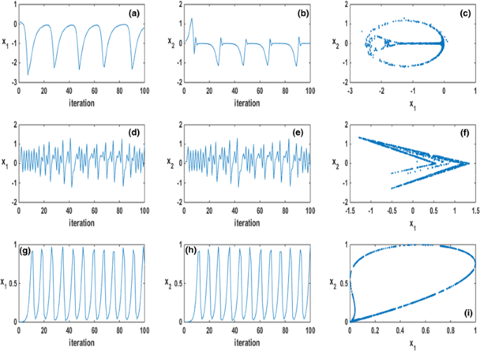

  

  Time-series and attractors of different chaotic maps: (a-c) Burger map, (d-f) Lozi map, and (g-i) Logistic map

• 2. Lozi map: this map can be mathematically expressed by:

  $$ \begin{aligned} \beta_{1} \left( {k + 1} \right) & = 1 - a.\beta_{1} \left( k \right) + b.\beta_{2} \left( k \right) \hfill \\ \beta_{2} \left( {k + 1} \right) & = \beta_{1} \left( k \right) \hfill \\ \end{aligned} $$

  (29)

  where the operating parameters a and b are equal to 1.7 and 0.5, respectively. Figure 7d–f indicate the attractor and time series of Lozi map for an initial condition β ₁ (0) = 0.1 and β ₂ (0) = 0.1.

• 3. Logistic map: this map can be mathematically indicated by:

  $$ \begin{aligned} \beta_{1} \left( {k + 1} \right) & = A.\beta_{1} \left( k \right)\left( {1 - \beta_{2} \left( k \right)} \right) \hfill \\ \beta_{2} \left( {k + 1} \right) & = \beta_{1} \left( k \right) \hfill \\ \end{aligned} $$

  (30)

  where the operating parameter A is equal to 2.27. Figure 7g–i indicate the attractor and time series of Logistic map for an initial condition β ₁ (0) = 0.001 and β ₂ (0) = 0.001.

The pseudo-code of CPSO with chaos is also depicted in Fig. 8.

Fig. 8

Algorithmic structure of the proposed solver

6 Results and discussion

This section is given into two subsections. In the first subsection, the steps required for fine tunings of the considered rival solvers and optimal controllers are discussed. The adopted performance evaluation metrics as well as the computational facilities used for the simulations are also presented. In the second subsection, the results of the numerical simulations are provided, and the obtained optimal controlling signals are used to regulate the performance of the considered engine over the coldstart period. Based on the presented results, it is demonstrated that the proposed intelligent optimal controller can cope with the nonlinearities associated with the operation of engine over the coldstart period.

6.1 Parameter settings and encoding procedure

For proceeding with the simulations, some parameter settings and setups should be done for both optimization and modeling modules. To ensure the efficient performance of ELM algorithm, a set of parametric studies is carried out. Through several trial-and-error efforts, the number of hidden nodes of 30 is used to form the hidden layer of ELM. Also, for the calculation of Tikhonov parameter, 10 different values are considered in the log-scale, and the BIC criterion suggests the use of the λ _T of 0.001 for this case study. The training process is conducted based on tenfold cross-validations in which the database is divided into 10 subgroups, and the experiments for each group are performed for 10 independent runs and then the average values are calculated. The average values of each of the tenfolds are again averaged and the final values are reported. To tune the parameters of ELM, 3 different experimentally collected signals are used for the estimations of T _exh and HC _raw which result in 6 different databases. The number of data points in each of the databases are 5001, 5001, 5001, 49209, 12001, and 12001, respectively, from which 80 % of the data points are used for the training/validation and the remaining 20 % data points are used for the testing phase. To evaluate the identification efficiency of ELM, the mean square error (MSE) metric is used. To evaluate the performance of the proposed optimization method as well as the solving algorithms, a number of rival techniques are taken into account. To demonstrate the computational power of CPSO with chaos (CPSO-C) for solving the system of equations resulting from the Hamiltonian function, a set of rival heuristic algorithms are considered. The rival optimization algorithms are PSO with inertia weight (PSO-w) [41], PSO with constriction factor (PSO-cf) [42], local version of PSO with inertia weight (PSO-w-local) [41], local version of PSO with constriction factor (PSO-cf-local) [42], unified PSO (UPSO) [43], fully informed PSO (FIPSO) [44], fitness distance ratio based PSO (FDPSO) [45], hybrid cooperative approach to PSO (CPSO-H) [46], and the standard cellular PSO (CPSO) [32]. Also, hereafter, CPSO with Lozi map, CPSO with Burger map, and CPSO with Logistic map are shown with CPSO-C-Loz, CPSO-C-Log, and CPSO-C-Burg, respectively. To mitigate the effects of the stochastic nature and randomness of the considered optimizers, and also, increase the reliability of the obtained results, the numerical experiments are executed for 30 independent runs with random initial seeds (based on the Monte-Carlo simulation). All of the algorithms transact the optimization procedure for 100,000 times of function evaluations (relatively equal to 1000 iteration). Also, to evaluate the exploration and exploitation capabilities and the power of the rival nature-inspired algorithms to converge to a unique solution, the convergence rate (CR) [33] metric is taken into account. The mathematical formulation of the CR is given below:

$$ fitness\,(ObjVal) = \left\{ \begin{aligned} \frac{1}{ObjVal + 1}\quad \quad ObjVal > 0 \hfill \\ \hfill \\ 1 + \left| {ObjVal} \right|\quad \quad ObjVal < 0 \hfill \\ \end{aligned} \right. $$

(31)

$$ Mean\;fitness = \frac{{\sum\limits_{i = 1}^{PopSize} {fitness(ObjVal(i))} }}{PopSize} $$

(32)

$$ Best\;fitness = \hbox{max} \left\{ {fitness(ObjVal(i))|\;i = 1, \ldots ,PopSize} \right\} $$

(33)

$$ CR = \frac{Mean\;fitness}{Best\;fitness} $$

(34)

Just like any other random procedure, it is necessary to find an expectation for the final value of CR with some initial conditions (for our case, the same initial seeding of the agents, which means an initial value of CR₀). The simulations are done for 30 runs, and E (CR|CR₀) is reported.

In general, the CR metric can take values within the range of unity [0, 1]. The CR value of 0 implies that the agents are completely diffused and there is a pure divergence, while the CR value of 1 indicates that the agents are converged to a unique solution state and the optimizer can neatly guide all of the agents towards the optimal solution. There is no doubt that the algorithmic functioning of standard PSO (and also most of its variants) forces the heuristic agents to converge to the same region with an increasing value of CR over the optimization procedure. We need to find out the speed of the convergence as well as the final CR value. Such elements are tested through the simulations to evaluate the performance of the rival methods.

It is necessary to present the encoding style required for solving the system of equations pertaining to the states, co-states, and controlling signals. As it was mentioned, there are 4 states, 4 co-states, and 2 controlling signals which should be optimally determined. These signals are discretized over 50 s, and by considering a time step of 1 s, each of these signals is divided and 500 nodal points are created which should be determined:

$$ {\mathbf{S}} = \left[ {\begin{array}{*{20}c} {{\mathbf{U}}^{*} \left( {k_{0} } \right)} & \cdots & {{\mathbf{U}}^{*} \left( {k_{f} } \right)} & {\begin{array}{*{20}c} {{\mathbf{X}}^{*} \left( {k_{0} } \right)} & \cdots & {{\mathbf{X}}^{*} \left( {k_{f} } \right)} & {\begin{array}{*{20}c} {\bar{\lambda }^{*} \left( {k_{0} } \right)} & \cdots & {\bar{\lambda }^{*} \left( {k_{f} } \right)} \\ \end{array} } \\ \end{array} } \\ \end{array} } \right] $$

(35)

Consider the system of equations obtained for the states, co-states, and controlling signals in Eqs. (A.1), (A.2), and (A.3), or in the compact form as stated in Eq. (22). Then, the decision variables should be obtained such that the functions below are minimized:

$$ \hbox{min} \left( \begin{aligned} \frac{{\partial {\mathbf{H}}\left( {{\mathbf{X}}^{*} \left( k \right),{\mathbf{U}}^{*} \left( k \right),\bar{\lambda }^{*} \left( {k + 1} \right)} \right)}}{{\partial x_{j}^{*} \left( k \right)}} + \lambda_{i}^{*} \left( k \right) + \frac{{\partial {\mathbf{H}}\left( {{\mathbf{X}}^{*} \left( k \right),{\mathbf{U}}^{*} \left( k \right),\bar{\lambda }^{*} \left( {k + 1} \right)} \right)}}{{\partial \lambda_{i}^{*} \left( k \right)}} - x_{j}^{*} \left( k \right) \hfill \\ \quad \quad \quad \quad \quad \quad + \frac{{\partial {\mathbf{H}}\left( {{\mathbf{X}}^{*} \left( k \right),{\mathbf{U}}^{*} \left( k \right),\bar{\lambda }^{*} \left( {k + 1} \right)} \right)}}{{\partial u_{q}^{*} \left( k \right)}} \hfill \\ \end{aligned} \right) $$

(36)

where i = 1, 2, 3, 4, j = 1, 3, 5, 6, and q = 1, 2. The system should be solved for k ₀ = 50 to k _f  = 50. A solver should try to minimize the above overall objective function. The following constraints also should be taken into account for the controlling signals (for each step-point during the control process):

$$ \left\{ \begin{aligned} & 40^{^\circ } \le u_{1} \left( k \right) \le 60^{^\circ } \hfill \\ & 10 \le u_{2} \left( k \right) \le 16 \hfill \\ \end{aligned} \right. $$

(37)

Furthermore, for assessing the performance of the proposed controller, which is, in fact, a CPSO based on fundamental theorem of calculus of variations optimal controller (CPSO-FT-OC), from now on, a classical optimal controller based on the Pontryagin’s minimum principle (PMP) [29] is also implemented for the same coldstart problem.

For the current simulations, three different pre-defined engine speed profiles (u ₃ ) are considered, which are depicted in Fig. 9.

Fig. 9

Considered engine speed profiles

All of the encodings, simulations, and numerical experiments are carried out in the Matlab software with Microsoft Windows 7 operating system on a PC with a Pentium IV, Intel core i7 CPU, and 4 GBs RAM.

6.2 Simulation results

Before proceeding with the control performance simulations, it is necessary to train the ELM to have a differentiable state-space representation of the system. Table 3 lists the training and testing errors for all of the six different cases. By comparing the obtained results with those from the model proposed in [8] versus the values obtained from a high-fidelity model developed at VDL lab, it can be easily inferred that the proposed differentiable neural model has an acceptable accuracy. It can be seen that for some of the cases, the estimation error is even less than the rival model. Figure 10 depicts the correlation results obtained using ELM. As can be seen, the estimation results and the measured ones are in a good agreement.

Table 3 Estimation error of ELM compared to the model developed in [8] for 3 different data sets versus values measured from a high-fidelity model

Fig. 10

Correlation plots obtained for the three different cases using ELM and those obtained from high fidelity model

The trained model is now used to derive the system of equations, which should be solved using the nature-inspired solvers. Here, the authors present the results of simulations regarding the calculation of optimal profiles using the rival optimization approaches. To capture the undesired effects of randomness and uncertainty, the simulations are repeated for 30 runs and the statistical results are presented in Tables 4, 5, and 6. By checking the obtained results, it can be seen that the cellular variants of PSO show much better results as compared to the other variants of PSO. Besides, the findings indicate that equipping the cellular transition rule with the chaos theory can further boost the performance. All in all, the obtained results demonstrate that CPSO-C-Burg and CPSO-C-Log can outperform the other rival methods. The std. values of all of the rival methods are relatively the same, which shows that all of the methods have an approximately similar robustness. The similar results are obtained for Cases 2 and 3; however, the difference pertains to the std. values of the rival methods. It is clear that the std. values of cellular variants of PSO are less than the other rival methods for the last two cases. Such observations bring the authors to the conclusion that, generally, the robustness of cellular PSO algorithms is more than the other rival methods. For the last two cases, the performance of CPSO-C-Burg is much better than the other rival methods, which suggests using this specific version of CPSO for the calculation of optimum controlling profiles. Figure 11 indicates the real-time evolution of the objective function, which results in a decrease of HC _cum . It can be seen that the final value for each case is different. In fact, the results show that, by increasing the engine speed, the value of HC _cum decreases. Such an observation is in a good agreement with the results of physical analysis reported in [47].

Table 4 Optimization results for the rival swam-based solvers for Case 1 for 30 independent runs

Table 5 Optimization results for the rival swam-based solvers for Case 2 for 30 independent runs

Table 6 Optimization results for the rival swam-based solvers for Case 3 for 30 independent runs

Fig. 11

Real-time evolution of the objective function obtained from CPSO-C-Burg

It is also necessary to evaluate the exploration/exploitation balance of the rival methods to find out whether the algorithms converge to a unique region with an acceptable quality. For this purpose, the performances of the rival methods are compared in terms of the convergence rate (CR) index. It is well-known that the standard PSO and most of its variants adaptively turn the exploration to an exploitation search. However, the key point is to find out whether a complete convergence occurs, and also, whether the method can optimally balance the exploration and exploitation capabilities to reach the CR value of 1 in a logical period of time. The speed of convergence is desirable if an algorithm can also converge to a solution with acceptable quality. Hence, the results of CR tests should be considered in tandem to the results of optimization performance. Figure 12a–c) indicates the real-time CR profiles for different optimization cases. To avoid any prejudice, all of the methods start the optimization with the same distribution of the agents corresponding to CR₀ of 0.1. As expected, all of the rival PSO variants have an increasing CR profile. However, it can be seen that CPSO and all of its variants can reach the CR value of 1 in a very short period of time. It can be also seen that FDPSO and PSO-w have acceptable convergence behavior over the optimization procedure. Figure 12d indicates the variation of CR profiles of CPSO-C-Burg for 4 independent runs. It can be seen that the obtained CR profiles have the relatively same path, and such an observation brings the authors to the conclusion that CPSO-C-Burg is robust in terms of the balance between exploration and exploitation capabilities. Given the results of this experiment and taking the accuracy experiment into account, one can easily infer that the performance of the CPSO-C-Burg is quite acceptable for solving the system of equations for the calculation of optimal profiles. The boxplots of the final obtained CR values of the rival methods over 30 independent runs are presented in Fig. 13. It can be seen that all of the considered methods show a trivial deviation of CR through the independent simulations. The results also reveal that PSO-cf-local and FIPSO do not have acceptable performances and their mean CR value is less than the other algorithms, which means that they often fail to converge to a unique solution through the independent runs.

Fig. 12

Real-time convergence profiles for: a Case 1, b Case 2, c Case 3, and d sensitivity of Burg-chaos-based CPSO for the three different cases over 4 independent runs

Fig. 13

Boxplots of the convergences of the rival methods for the three considered cases

Finally, the optimal control effort surfaces obtained by CPSO-C-Burg are given in Fig. 14. It can be seen that the overall shapes of the obtained surfaces are equal for the three controlling cases. However, it can be seen that the surfaces of Cases 2 and 3 cover a broader range with respect to the AFR control signal. The optimal state surfaces are also presented in Fig. 15. The differences of the calculated states are clear, and it can be seen that there is a remarkable difference when a surface is presented in terms of X₆.

Fig. 14

Different surfaces of the control efforts calculated by the optimal controller

Fig. 15

Different surfaces of the states calculated by the optimal controller

Figure 16 indicates the variations of exhaust gas temperature for the three cases with respect to the controlling signals. It is clear that the final value of T_exh profile is higher for the last case, and it is the lowest for Case 1. Such observations bring us to the conclusion that increasing the engine speed has a positive impact on the exhaust gas temperature. The relatively same behavior is observed for the engine-out hydrocarbon emissions (HC _raw-c ) (as indicated in Fig. 17). The catalytic converter efficiency profiles are also presented in Fig. 18. It can be seen that, for Case 1, the catalyst’s efficiency reaches the nominal value in a shorter period of time (in 20 s), and the required time for the same phenomenon is about 35 s for Case 3 which has the lowest engine speed profile.

Fig. 16

Variations of T _exh with respect to: a spark timing, and b air/fuel ratio

Fig. 17

Variations of HC _raw with respect to a spark timing, and b air/fuel ratio

Fig. 18

Catalytic converter efficiency profiles for the three cases

As an optimal controller, the performance of the proposed controller should also be compared with another high-performance rival method. In a previous work by the authors’ research group, it was demonstrated that PMP can show very promising result for the coldstart problem. Here, the authors compare their controller with the results obtained using PMP. The comparative results are presented in Table 7. It can be seen that the results of the proposed controller is acceptable as compared to those of PMP (which is among the most powerful optimal controllers). It can be seen that for Case 3, the obtained result is remarkably better than PMP, and for the other cases, the obtained results are comparable. Moreover, it is obvious that the proposed intelligent controller has a neural network at its heart which can neatly deal with disturbances and noises in practice as it can be retrained, if necessary, to increase the accuracy of the calculated controlling profiles.

Table 7 Comparison of the results obtained by PMP and CPSO-FT-OC

7 Concluding remarks

In this study, for an automotive engine during the coldstart period, a novel intelligent optimal control scheme was proposed using the Hamiltonian function, to formulate the objective function based on the engine system’s state-space model and an approximation method, known as extreme learning machine (ELM). ELM was used to estimate the values of exhaust gas temperature (T _exh ) and engine-out hydrocarbon emissions (HC _raw-c ) using the state values coming from a control-oriented model of the system. By formulating the nonlinear state, co-state and control input equations for the coldstart problem, a large-scale constraint optimization problem emerged which was solved by a cellular particle swarm optimization (CPSO) algorithm. The simulation results clearly demonstrated that the method is best suited for the calculation of the optimal controlling and state profiles for the considered problem. Indeed, the power of the optimization method enabled us to consider different operating cases and come up with practical results. Furthermore, the continuous differentiable formulation of ELM allowed us to develop some representative formulations for T _exh and HC _raw-c to calculate the optimal values based on the fundamental theorem of calculus of variations. To further demonstrate the efficacy of the proposed controller, as well as CPSO, different rival population-based solvers and also a powerful optimal controller based on the Pontryagin’s minimum principle (PMP) were taken into account. The results of the comparative study clearly demonstrated the efficacy and feasibility of the controlling commands obtained by the proposed intelligent optimal controller. The results also brought the authors to the conclusion that the adopted CPSO can yield a qualified solution compared to the other rival techniques. In general, our findings show that the proposed intelligent controller is best suited for the considered problem, which is one of the most critical issues from the automotive industry’s perspective.

Appendix A

Details of difference-based formulations of the proposed controller

The following difference-based system of equations is obtained for the co-states:

$$ \,\left\{ \begin{array}{l} \frac{{\partial {\mathbf{H}}\left( {{\mathbf{X}}^{*} \left( k \right),{\mathbf{U}}^{*} \left( k \right),\bar{\lambda }^{*} \left( {k + 1} \right)} \right)}}{{\partial x_{1}^{*} \left( k \right)}} = - \lambda_{1}^{*} \left( k \right) \hfill \\ \quad = - \,\,K_{{T_{exh} }} \sum\limits_{j = 1}^{N} {\left( {\omega_{j}^{1} {\kern 1pt} \frac{{\partial {\kern 1pt} g\left( {\alpha_{j}^{1} \Im_{1} \left( k \right) + \alpha_{j}^{2} \Im_{2} \left( k \right) + \alpha_{j}^{3} \Im_{1} \left( k \right) + b_{j}^{1} } \right)}}{{\partial {\kern 1pt} \Im_{1} \left( k \right)}} \cdot \frac{{\partial {\kern 1pt} \Im_{1} \left( k \right)}}{{\partial x_{1}^{*} \left( k \right)}}} \right)} - \left( {\frac{{k_{1} }}{{\tau_{1} }}\lambda_{1}^{*} \left( {k + 1} \right)} \right) \hfill \\ \frac{{\partial {\mathbf{H}}\left( {{\mathbf{X}}^{*} \left( k \right),{\mathbf{U}}^{*} \left( k \right),\bar{\lambda }^{*} \left( {k + 1} \right)} \right)}}{{\partial x_{3}^{*} \left( k \right)}} = - \lambda_{2}^{*} \left( k \right) \hfill \\ \quad = - \,K_{{T_{exh} }} \sum\limits_{j = 1}^{N} {\left( {\omega_{j}^{1} {\kern 1pt} \frac{{\partial {\kern 1pt} g\left( {\alpha_{j}^{1} \Im_{1} \left( k \right) + \alpha_{j}^{2} \Im_{2} \left( k \right) + \alpha_{j}^{3} \Im_{1} \left( k \right) + b_{j}^{1} } \right)}}{{\partial {\kern 1pt} \Im_{3} \left( k \right)}} \cdot \frac{{\partial {\kern 1pt} \Im_{3} \left( k \right)}}{{\partial x_{3}^{*} \left( k \right)}}} \right)} - \left( {\frac{{k_{3} }}{{\tau_{3} }}\lambda_{2}^{*} \left( {k + 1} \right)} \right) \hfill \\ \frac{{\partial {\mathbf{H}}\left( {{\mathbf{X}}^{*} \left( k \right),{\mathbf{U}}^{*} \left( k \right),\bar{\lambda }^{*} \left( {k + 1} \right)} \right)}}{{\partial x_{5}^{*} \left( k \right)}} = - \lambda_{3}^{*} \left( k \right) = \hfill \\ \quad = \;\;K_{HC} \sum\limits_{j = 1}^{N} {\left( {\omega_{j}^{2} {\kern 1pt} \frac{{\partial {\kern 1pt} g\left( {\kappa_{j}^{1} \Im_{4} \left( k \right) + \kappa_{j}^{2} \Im_{5} \left( k \right) + \kappa_{j}^{3} \Im_{6} \left( k \right) + b_{j}^{2} } \right)}}{{\partial {\kern 1pt} \Im_{5} \left( k \right)}} \cdot \frac{{\partial {\kern 1pt} \Im_{5} \left( k \right)}}{{\partial x_{5}^{*} \left( k \right)}}} \right)} - \left( {\frac{{k_{5} }}{{\tau_{5} }}\lambda_{3}^{*} \left( {k + 1} \right)} \right) \hfill \\ \frac{{\partial {\mathbf{H}}\left( {{\mathbf{X}}^{*} \left( k \right),{\mathbf{U}}^{*} \left( k \right),\bar{\lambda }^{*} \left( {k + 1} \right)} \right)}}{{\partial x_{6}^{*} \left( k \right)}} = - \lambda_{4}^{*} \left( k \right) = \hfill \\ \quad = \;\;K_{HC} \sum\limits_{j = 1}^{N} {\left( {\omega_{j}^{2} {\kern 1pt} \frac{{\partial {\kern 1pt} g\left( {\kappa_{j}^{1} \Im_{4} \left( k \right) + \kappa_{j}^{2} \Im_{5} \left( k \right) + \kappa_{j}^{3} \Im_{6} \left( k \right) + b_{j}^{2} } \right)}}{{\partial {\kern 1pt} \Im_{6} \left( k \right)}} \cdot \frac{{\partial {\kern 1pt} \Im_{6} \left( k \right)}}{{\partial x_{6}^{*} \left( k \right)}}} \right)} - \left( {\frac{{k_{6} }}{{\tau_{6} }}\lambda_{4}^{*} \left( {k + 1} \right)} \right) \hfill \\ \end{array} \right. $$

(A.1)

Moreover, the following difference-based system of equations is obtained for the states:

$$ \,\left\{ \begin{array}{l} \frac{{\partial {\mathbf{H}}\left( {{\mathbf{X}}^{*} \left( k \right),{\mathbf{U}}^{*} \left( k \right),\bar{\lambda }^{*} \left( {k + 1} \right)} \right)}}{{\partial \lambda_{1}^{*} \left( {k + 1} \right)}} = x_{1}^{*} \left( {k + 1} \right) = \delta t \cdot \frac{{u_{1} \left( k \right)}}{{\tau_{1} }} + \left( {1 - \frac{{\delta t \cdot k_{1} }}{{\tau_{1} }}} \right)x_{1} \left( k \right) \hfill \\ \frac{{\partial {\mathbf{H}}\left( {{\mathbf{X}}^{*} \left( k \right),{\mathbf{U}}^{*} \left( k \right),\bar{\lambda }^{*} \left( {k + 1} \right)} \right)}}{{\partial \lambda_{2}^{*} \left( {k + 1} \right)}} = x_{3}^{*} \left( {k + 1} \right) = \delta t \cdot \frac{{16 - u_{2} \left( k \right)}}{{\tau_{3} }} + \left( {1 - \frac{{\delta t \cdot k_{3} }}{{\tau_{3} }}} \right)x_{3} \left( k \right) \hfill \\ \frac{{\partial {\mathbf{H}}\left( {{\mathbf{X}}^{*} \left( k \right),{\mathbf{U}}^{*} \left( k \right),\bar{\lambda }^{*} \left( {k + 1} \right)} \right)}}{{\partial \lambda_{3}^{*} \left( {k + 1} \right)}} = x_{5}^{*} \left( {k + 1} \right) = \delta t \cdot \frac{{16 - u_{2} \left( k \right)}}{{\tau_{5} }} + \left( {1 - \frac{{\delta t \cdot k_{5} }}{{\tau_{5} }}} \right)x_{5} \left( k \right) \hfill \\ \frac{{\partial {\mathbf{H}}\left( {{\mathbf{X}}^{*} \left( k \right),{\mathbf{U}}^{*} \left( k \right),\bar{\lambda }^{*} \left( {k + 1} \right)} \right)}}{{\partial \lambda_{4}^{*} \left( {k + 1} \right)}} = x_{6}^{*} \left( {k + 1} \right) = \delta t \cdot \frac{{\left| {u_{1} \left( k \right) - 55} \right| + \left( {u_{1} \left( k \right) - 55} \right)}}{{2\tau_{6} }} + \left( {1 - \frac{{\delta t \cdot k_{6} }}{{\tau_{6} }}} \right)x_{6} \left( k \right) \hfill \\ \end{array} \right. $$

(A.2)

In addition, the following equations are derived for the control signals:

$$ \,\left\{ \begin{aligned} \frac{{\partial {\mathbf{H}}\left( {{\mathbf{X}}^{*} \left( k \right),{\mathbf{U}}^{*} \left( k \right),\bar{\lambda }^{*} \left( {k + 1} \right)} \right)}}{{\partial u_{1}^{*} \left( {k + 1} \right)}} = 0 = K_{HC} \sum\limits_{j = 1}^{N} {\left( {\omega_{j}^{2} {\kern 1pt} \frac{{\partial {\kern 1pt} g\left( {\kappa_{j}^{1} \Im_{4} \left( k \right) + \kappa_{j}^{2} \Im_{5} \left( k \right) + \kappa_{j}^{3} \Im_{6} \left( k \right) + b_{j}^{2} } \right)}}{{\partial {\kern 1pt} \Im_{6} \left( k \right)}} \cdot \frac{{\partial {\kern 1pt} \Im_{6} \left( k \right)}}{{\partial u_{1}^{*} \left( k \right)}}} \right)} \hfill \\ \quad \quad \quad \quad \quad \quad \quad \quad \quad \quad \quad \quad \quad \quad \quad - K_{{T_{exh} }} \sum\limits_{j = 1}^{N} {\left( {\omega_{j}^{1} {\kern 1pt} \frac{{\partial {\kern 1pt} g\left( {\alpha_{j}^{1} \Im_{1} \left( k \right) + \alpha_{j}^{2} \Im_{2} \left( k \right) + \alpha_{j}^{3} \Im_{3} \left( k \right) + b_{j}^{1} } \right)}}{{\partial {\kern 1pt} \Im_{1} \left( k \right)}} \cdot \frac{{\partial {\kern 1pt} \Im_{1} \left( k \right)}}{{\partial u_{1}^{*} \left( k \right)}}} \right)} \hfill \\ \quad \quad \quad \quad \quad \quad \quad \quad \quad + \frac{{\lambda_{1}^{*} \left( {k + 1} \right)}}{{\tau_{1} }} + \frac{{\lambda_{4}^{*} \left( {k + 1} \right)}}{{2\tau_{6} }}\left( {1 + \frac{1}{{\left| {u_{1}^{*} \left( k \right) - 55} \right|}}} \right) \hfill \\ \frac{{\partial {\mathbf{H}}\left( {{\mathbf{X}}^{*} \left( k \right),{\mathbf{U}}^{*} \left( k \right),\bar{\lambda }^{*} \left( {k + 1} \right)} \right)}}{{\partial u_{2}^{*} \left( {k + 1} \right)}} = 0 = K_{HC} \sum\limits_{j = 1}^{N} {\left( {\omega_{j}^{2} {\kern 1pt} \frac{{\partial {\kern 1pt} g\left( {\kappa_{j}^{1} \Im_{4} \left( k \right) + \kappa_{j}^{2} \Im_{5} \left( k \right) + \kappa_{j}^{3} \Im_{6} \left( k \right) + b_{j}^{2} } \right)}}{{\partial {\kern 1pt} \Im_{5} \left( k \right)}} \cdot \frac{{\partial {\kern 1pt} \Im_{5} \left( k \right)}}{{\partial u_{2}^{*} \left( k \right)}}} \right)} \hfill \\ \quad \quad \quad \quad \quad \quad \quad \quad \quad \quad \quad \quad \quad \quad \quad - K_{{T_{exh} }} \sum\limits_{j = 1}^{N} {\left( {\omega_{j}^{1} {\kern 1pt} \frac{{\partial {\kern 1pt} g\left( {\alpha_{j}^{1} \Im_{1} \left( k \right) + \alpha_{j}^{2} \Im_{2} \left( k \right) + \alpha_{j}^{3} \Im_{3} \left( k \right) + b_{j}^{1} } \right)}}{{\partial {\kern 1pt} \Im_{3} \left( k \right)}} \cdot \frac{{\partial {\kern 1pt} \Im_{3} \left( k \right)}}{{\partial u_{2}^{*} \left( k \right)}}} \right)} \hfill \\ \quad \quad \quad \quad \quad \quad + \frac{{\lambda_{2}^{*} \left( {k + 1} \right)}}{{\tau_{3} }} + \frac{{\lambda_{3}^{*} \left( {k + 1} \right)}}{{2\tau_{5} }} \hfill \\ \end{aligned} \right. $$

(A.3)

For Eqs. (A.1) to (A.3), the following differentiations should be employed:

$$ \begin{array}{l} \frac{{\partial {\kern 1pt} g\left( {\alpha_{j}^{1} \Im_{1} \left( k \right) + \alpha_{j}^{2} \Im_{2} \left( k \right) + \alpha_{j}^{3} \Im_{3} \left( k \right) + b_{j}^{1} } \right)}}{{\partial {\kern 1pt} \Im_{1} \left( k \right)}} = \frac{{\alpha_{j}^{1} \cdot e^{{ - \left( {\alpha_{j}^{1} \Im_{1} \left( k \right) + \alpha_{j}^{2} \Im_{2} \left( k \right) + \alpha_{j}^{3} \Im_{3} \left( k \right) + b_{j}^{1} } \right)}} }}{{\left( {1 + e^{{ - \left( {\alpha_{j}^{1} \Im_{1} \left( k \right) + \alpha_{j}^{2} \Im_{2} \left( k \right) + \alpha_{j}^{3} \Im_{3} \left( k \right) + b_{j}^{1} } \right)}} } \right)^{2} }} \hfill \\ \frac{{\partial {\kern 1pt} g\left( {\alpha_{j}^{1} \Im_{1} \left( k \right) + \alpha_{j}^{2} \Im_{2} \left( k \right) + \alpha_{j}^{3} \Im_{3} \left( k \right) + b_{j}^{1} } \right)}}{{\partial {\kern 1pt} \Im_{3} \left( k \right)}} = \frac{{\alpha_{j}^{3} \cdot e^{{ - \left( {\alpha_{j}^{1} \Im_{1} \left( k \right) + \alpha_{j}^{2} \Im_{2} \left( k \right) + \alpha_{j}^{3} \Im_{3} \left( k \right) + b_{j}^{1} } \right)}} }}{{\left( {1 + e^{{ - \left( {\alpha_{j}^{1} \Im_{1} \left( k \right) + \alpha_{j}^{2} \Im_{2} \left( k \right) + \alpha_{j}^{3} \Im_{3} \left( k \right) + b_{j}^{1} } \right)}} } \right)^{2} }} \hfill \\ \frac{{\partial {\kern 1pt} g\left( {\kappa_{j}^{1} \Im_{4} \left( k \right) + \kappa_{j}^{2} \Im_{5} \left( k \right) + \kappa_{j}^{3} \Im_{6} \left( k \right) + b_{j}^{2} } \right)}}{{\partial {\kern 1pt} \Im_{5} \left( k \right)}} = \frac{{\kappa_{j}^{2} \cdot e^{{ - \left( {\kappa_{j}^{1} \Im_{4} \left( k \right) + \kappa_{j}^{2} \Im_{5} \left( k \right) + \kappa_{j}^{3} \Im_{6} \left( k \right) + b_{j}^{2} } \right)}} }}{{\left( {1 + e^{{ - \left( {\kappa_{j}^{1} \Im_{4} \left( k \right) + \kappa_{j}^{2} \Im_{5} \left( k \right) + \kappa_{j}^{3} \Im_{6} \left( k \right) + b_{j}^{2} } \right)}} } \right)^{2} }} \hfill \\ \frac{{\partial {\kern 1pt} g\left( {\kappa_{j}^{1} \Im_{4} \left( k \right) + \kappa_{j}^{2} \Im_{5} \left( k \right) + \kappa_{j}^{3} \Im_{6} \left( k \right) + b_{j}^{2} } \right)}}{{\partial {\kern 1pt} \Im_{6} \left( k \right)}} = \frac{{\kappa_{j}^{3} \cdot e^{{ - \left( {\kappa_{j}^{1} \Im_{4} \left( k \right) + \kappa_{j}^{2} \Im_{5} \left( k \right) + \kappa_{j}^{3} \Im_{6} \left( k \right) + b_{j}^{2} } \right)}} }}{{\left( {1 + e^{{ - \left( {\kappa_{j}^{1} \Im_{4} \left( k \right) + \kappa_{j}^{2} \Im_{5} \left( k \right) + \kappa_{j}^{3} \Im_{6} \left( k \right) + b_{j}^{2} } \right)}} } \right)^{2} }} \hfill \\ \frac{{\partial {\kern 1pt} \Im_{1} \left( k \right)}}{{\partial x_{1}^{*} \left( k \right)}} = 1 - \frac{{\delta t \cdot k_{1} }}{{\tau_{1} }};\quad \frac{{\partial {\kern 1pt} \Im_{3} \left( k \right)}}{{\partial x_{3}^{*} \left( k \right)}} = 1 - \frac{{\delta t \cdot k_{3} }}{{\tau_{3} }};\quad \frac{{\partial {\kern 1pt} \Im_{5} \left( k \right)}}{{\partial x_{5}^{*} \left( k \right)}} = 1 - \frac{{\delta t \cdot k_{5} }}{{\tau_{5} }} \hfill \\ \frac{{\partial {\kern 1pt} \Im_{6} \left( k \right)}}{{\partial x_{6}^{*} \left( k \right)}} = 1 - \frac{{\delta t \cdot k_{6} }}{{\tau_{6} }};\quad \frac{{\partial {\kern 1pt} \Im_{1} \left( k \right)}}{{\partial u_{1}^{*} \left( k \right)}} = \frac{\delta t}{{\tau_{1} }};\quad \frac{{\partial {\kern 1pt} \Im_{6} \left( k \right)}}{{\partial u_{1}^{*} \left( k \right)}} = \frac{\delta t}{{2\tau_{6} }}\left( {1 + \frac{1}{{\left| {u_{1} \left( k \right) - 55} \right|}}} \right) \hfill \\ \frac{{\partial {\kern 1pt} \Im_{3} \left( k \right)}}{{\partial u_{2}^{*} \left( k \right)}} = \frac{ - \delta t}{{\tau_{3} }};\quad \frac{{\partial {\kern 1pt} \Im_{5} \left( k \right)}}{{\partial u_{2}^{*} \left( k \right)}} = \frac{ - \delta t}{{\tau_{5} }} \hfill \\ \end{array} $$

References

Rajmani R (2012) Vehicle dynamics and control. Springer-Verlag, Mech Eng Series
Taghavipour A, Azad NL, McPhee J (2015) Real-time predictive control strategy for a plug-in hybrid electric powertrain. Mechatronics. doi:10.1016/j.mechatronics.2015.04.020
Ulsoy AG, Peng H, Cakmakci M (2014) Automotive control systems. Cambridge Press, Cambridge
Zhai YJ, Yu DL (2009) Neural network model-based automotive engine air/fuel ratio control and robustness evaluation. Eng Appl Artif Intell 22:171–180
Taghavipour A, Azad NL, McPhee J (2012) An optimal power management strategy for power-split plug-in hybrid electric vehicles. Int J Veh Des 60(3/4):286–304
Asadi B, Vahidi A (2011) Predictive cruise control: utilizing upcoming traffic signal information for improving fuel economy and reducing trip time. IEEE Trans Control Syst Technol 19(3):707–714
Xiao L, Gao F (2010) A comprehensive review of the development of adaptive cruise control systems. Veh Syst Dyn 48(10):1167–1192
Azad NL, Sanketi PR, Hedrick JK (2012) Determining model accuracy requirements for automotive engine coldstart hydrocarbon emissions control. J Dyn Syst T ASME 134(5):051002
Vajedi M, Azad NL (2014) Ecological adaptive cruise controller for plug-in hybrid electric vehicles using nonlinear model predictive control. IEEE Trans Intell Trans Syst. doi:10.1109/TITS.2015.2462843
Qin G, Ge A, Lee JJ (2006) Fuzzy logic control for automobiles I: knowledge-based gear position decision. Adv Ind, Control, pp 145–157
Chen X, Wang Y, Haskara I, Zhu G (2014) Optimal air-to-fuel ratio tracking control with adaptive biofuel content estimation for LNT regeneration. IEEE Trans Contr Sys Tech 22(2):428–439
Cheng X, Jiang S, Wang S (2011) Design of a sliding mode controller for automotive engine speed regulation. In: IEEE Conference Industrial Electronics and Applications, Beijing, pp 1722–1725
Mozaffari A, Vajedi M, Azad NL (2015) A robust safety-oriented autonomous cruise control scheme for electric vehicles based on model predictive control and online sequential extreme learning machine with a hyper-level fault tolerance-based supervisor. Neurocomputing 151(2):845–856
Salehi R, Shahbakhti M, Hedrick JK (2014) Real-time hybrid switching control of automotive cold start hydrocarbon emission. J Dyn Syst T ASME 136:041002
Dextreit C, Kolmonovsky IV (2014) Game theory controller for hybrid electric vehicles. IEEE Trans Contr Sys Tech 22(2):652–663
Azad NL, Khajepour A, McPhee J (2007) Robust state feedback stabilization of articulated steer vehicles. Vehicle Syst Dyn 45(3):249–275
Zhang S, Zhang C, Han G, Wang Q (2014) Optimal control strategy design based on dynamic programming for a dual-motor coupling-propulsion system, Sci World J 2014: Article ID: 958239
Prokhorov DV (2008) Computational intelligence in automotive applications. Studies in Computational Intelligence. Springer-Verlag, Berlin
Zavala JC (2007) Engine modeling and control for minimization of hydrocarbon coldstart emissions in SI engine. Ph.D. Thesis, University of California, Berkeley, USA
Sanketi PR, Zavala JC, Hedrick JK (2006) Automotive engine hybrid modeling and control for reduction of hydrocarbon emissions. Int J Control 79(5):449–464
Wittka T, Muller V, Dittmann P, Pischinger S (2015) Development and investigation of diesel fuel reformer for LNT regeneration. Emiss Control Sci Technol. doi:10.1007/s40825-015-0017-8
Brijesh P, Sreedhara S (2013) Exhaust emissions and its control methods in compression ignition engines: a review. Int J Auto Tech-Kor 14(2):195–206
Shaw B, Hedrick JK (2003) Closed-loop engine coldstart control to reduce hydrocarbon emissions, American Control Conference 1392–1397
Sanketi PR, Zavala JC, Wilcutts M, Kaga T, Hedrick JK (2007) MIMO control for automotive coldstart. Fifth IFAC Symposium on Advances in Automotive Control, August
Zavala JC, Sanketi PR, Wilcutts M, Kaga T, Hedrick JK (2007) Simplified models of engine HC emissions, exhaust temperature and catalyst temperature for automotive coldstart, Fifth IFAC Symposium on Advances in Automotive Control, August
Mozaffari A, Azad NL (2014) Optimally pruned extreme learning machine with ensemble of regularization techniques and negative correlation penalty applied to automotive engine coldstart hydrocarbon emission identification. Neurocomputing 131:143–156
Mozaffari A, Azad NL (2014) A robust time delay auto-regressive exogenous fuzzy inference system for real-time estimation of catalyst temperature over engines coldstart operation: a multiobjective implementation scenario. Int J Dyn Control. doi:10.1007/s40435-014-0133-2
Mozaffari A, Azad NL (2015) Coupling Gaussian generalised regression neural network and mutable smart bee algorithm to analyse the characteristics of automotive engine coldstart hydrocarbon emission. J Exp Theor Artif Intell 27(3):253–272
Naidu DS (2003) Optimal control systems. CRC Press
Huang GB, Wang DH, Lan Y (2011) Extreme learning machines: a survey. Int J Mach Learn Cybern 2:107–122
Hastie T, Tibshirani R, Friedman J (2008) The elements of statistical learning: data mining, inference, and prediction, Springer Series in Statistics
Shi Y, Liu H, Gao L, Zhang G (2011) Cellular particle swarm optimization. Inf Sci 181:4460–4493
Fathi A, Mozaffari A (2014) Modeling a shape memory alloy actuator using an evolvable recursive black-box and hybrid heuristic algorithms inspired based on the annual migration of salmons in nature. Appl Soft Comput 14:229–251
Poli R, Kennedy J, Blackwell T (2007) Particle swarm optimization. Swarm Intell 1(1):33–57
Mozaffari A, Behzadipour S (2015) A modular extreme learning machine with linguistic interpreter and accelerated chaotic distributor for evaluating the safety of robot maneuvers in laparoscopic surgery. Neurocomputing 151(2):913–932
Emami M, Mozaffari A, Azad NL, Rezaie B (2014) An empirical investigation into the effects of chaos on different types of evolutionary crossover operators for efficient global search in complicated landscapes. Int J Comput Math. doi:10.1080/00207160.2014.985664
Mozaffari A, Emami M, Azad NL, Fathi A (2014) On the efficacy of chaos-enhanced heuristic walks with nature-based controllers for robust and accurate intelligent search, part A: an experimental analysis. J Exp Theor Artif Intell. doi:10.1080/0952813X.2014.954632
Metlicka M, Davendra D (2015) Chaos driven discrete artificial bee algorithm for location and assignment optimisation problems. Swarm Evol Comput. doi:10.1016/j.swevo.2015.03.002
Gandomi A, Yang XS (2014) Chaotic bat algorithm. J Comput Sci 5(2):224–232
Zelinka I, Celikovsky S, Richter H, Chen G (2010) Evolutionary algorithms and chaotic systems, studies in computational intelligence
Shi Y, Eberhart RC (1998) A modified particle swarm optimizer. Proc IEEE Int Conf Evol Comput Anchorage Alaska 1998:66–73
Clerc M, Kennedy J (2002) The particle swarm-explosion, stability, and convergence in a multidimensional complex space. IEEE Trans Evol Comput 6:58–73
Parsopoulos KE, Vrahatis MN (2004) UPSO: a unified particle swarm optimization scheme, Lecture Series on Computational Sciences, pp 868–873
Mendes R, Kennedy J, Neves J (2004) The fully informed particle swarm: simpler, maybe better. IEEE Trans Evol Comput 8:204–210
Peram T, Veeramachaneni K, Mohan CK (2003) Fitness–distance-ratio based particle swarm optimization, Proceedings of Swarm Intelligence Symposium, pp 174–181
Van den Bergh F, Engelbrecht AP (2004) A cooperative approach to particle swarm optimization. IEEE Trans Evol Comput 8(3):225–239
Azad NL (2015) On-line optimization of automotive engine coldstart hydrocarbon emissions control at idle conditions. Proc IMechE I J Sys Contr Eng 229(9):781–796
Mozaffari A (2015) Predictive control strategies for automotive engine coldstart emissions. MSc. Thesis, University of Waterloo, http://hdl.handle.net/10012/9673
Wong PK, Wong HC, Vong CM, Long TM, Wong KI, Gao X (2015) Fault tolerance automotive air-ratio control using extreme learning machine model predictive controller, Math Probl Eng 2015, Article ID: 317142
Vaughan A, Bohac SV (2015) Real-time, adaptive machine learning for non-stationary, near chaotic gasoline engine combustion time series. Neural Netw 70:18–26
Janakiraman VM, Nguyen XL, Sterniak J, Assanis D (2015) Identification of the dynamic operating envelope of HCCI engines using class imbalance learning. IEEE Trans Neural Netw Learn Syst 26(1):98–112
Wong PK, Wong KI, Vong CM, Cheung CS (2015) Modeling and optimization of biodiesel engine performance using kernel-based extreme learning machine and cuckoo search. Renew Energ 74:640–647
Wong KI, Vong CM, Wong PK, Luo J (2015) Sparse Bayesian extreme learning machine and its application to biofuel engine performance prediction. Neurocomputing 149:397–404
Wong PK, Vong CM, Gao XH, Wong KI (2014) Adaptive control using fully online sequential-extreme learning machine and a case study on engine air-fuel Ratio regulation, Math Probl Eng 2014, Article ID: 246964
Mozaffari A, Azad NL, Hedrick JK (2015) A hybrid switching predictive controller based on bi-level kernel-based ELM and online trajectory builder for automotive coldstart emissions reduction. Neurocomputing. doi:10.1016/j.neucom.2015.08.070
Wong PK, Wong HC, Vong CM, Xie Z, Huang S (2015) Model predictive engine air-ratio control using online sequential extreme learning machine. Neural Comput Appl. doi:10.1007/s00521-014-1555-7
Shaw B (2002) Modeling and control of automotive coldstart hydrocarbon emissions. Ph.D. Thesis, University of California, Berkeley, USA
Author information
Authors and Affiliations
Corresponding author