Efficient approaches to optimize energy consumption in 3D wireless video sensor network under the coverage and connectivity constraints

Abstract

Two advanced approaches (PA_1, and PA_2) based on a realistic 3D model of video sensor nodes (VSNs) deployed randomly over a 2D target area are proposed to minimize energy consumption in the network maintaining area coverage and connectivity. The reduction of the number of active VSNs decreases energy consumption but at the same time reduces the area coverage and connectivity. These conflicting issues are resolved and an optimal solution is obtained by using an integer linear programming-based approach (PA_1). But PA_1 is not tractable for large instances as the problem is NP-Hard. Hence, a heuristic approach (PA_2) based on an advanced genetic algorithm is also proposed in the present work for obtaining a near-optimal solution. Simulation studies are carried out to compare the performance of PA_1 and PA_2 with the other three state-of-the-art approaches (APP_5, APP_6, and ET_3). Among the three existing approaches, APP_6/(ET_3) is the best in energy consumption/(area coverage). It is observed that for the same simulation environment, both PA_1 and PA_2 guarantee higher network services, by reducing energy consumption by 40.85% and 33.34% respectively compared to the best existing approach APP_6; and as well as by increasing area coverage by 0.94% than the best existing approach ET_3 for the node density 150 on the target area of size 75x75 square meter. Between PA_1 and PA_2, PA_2 generates a suboptimal solution and PA_1 substantiates its superiority by reducing energy consumption by 11.26% than PA_2 without losing area coverage for the same simulation environment.

1 Introduction

A set of video sensor nodes (VSNs) furnished with miniature video cameras called CMOS [1, 2] cameras forms a wireless video sensor network (WVSN). Such sensors possess the function of capturing video and images and are extensively utilized in various applications like surveillance work, monitoring in the affected area with natural disasters, tracking, environment monitoring, etc. Operational by limited battery power, WVSN exhibits its challenging attitude in the profile of energy consumption as in almost all the cases the battery is not rechargeable, nor it is replaceable. Such VSNs can exhaust energy rapidly owing to constant sensing and transmission of video data. It lowers both monitoring quality and network lifetime.

The WVSN generally operates in an unfriendly environment, which requires VSNs to be deployed randomly with high density to ensure the smooth working of the application even if a few VSNs fail. But such densely deployed VSNs generate huge overlapping of coverage in the target area. The scheduling schemes of [1,2,3,4,5,6,7,8,9] utilize such overlapping coverage to cover the sensing area/region of a VSN and to shut such VSNs off for lowering the number of active VSNs which results in the reduction of energy consumption in the target area, without losing the percentage of initial area coverage by the VSNs significantly (termed as coverage constraint). But, the minimization (optimization) of the number of active VSNs (or, minimization of energy consumption by the active VSNs) is not addressed in [1,2,3,4,5,6,7,8,9]. Moreover, the connectivity among VSNs and between VSN and the base station (BS) (termed as connectivity constraints) are not addressed in [1,2,3,4,5,6,7,8,9]. The issue of minimizing the number of active VSNs (or energy consumption in the target area) while satisfying coverage constraint and also connectivity constraints is addressed by proposing new approaches (PA_1, PA_2) in this work. Both approaches use the 3D coverage model of VSNs.

PA_1 uses a single-objective optimization technique Integer Linear Program (ILP) for a system of linear constraints, with the objective to minimize the total number of active 3D VSNs for a particular random distribution of 3D VSNs. ILP generates the optimal solution but is intractable for large instances as the problem is NP-Hard [10]. PA_2, a heuristic approach based on the Advanced Genetic Algorithm (AGA) [11, 12] solves the same problem to produce the near-optimal solution, which runs in polynomial time and provides the solution for a large problem size.

A single base station (BS) is set up by the side of the target area both in PA_1 and PA_2 and the location of the BS in the target area is supplied to all the VSNs before their deployment. The BS is connected to WVSN via some VSNs that are inside the communication range of the BS. Each VSN in both approaches executes the neighbor discovery phase, registration phase, and duty cycling phase sequentially in the target area. In the neighbor discovery phase, each VSN identifies the position and also orientation of its neighbor VSNs by exchanging messages among themselves. It then inserts such neighbor information in a neighbor table both in PA_1 and PA_2. In the phase of registration, each VSN in both PA_1 and PA_2 transmits its position and orientation for itself to the BS. The BS inserts such type of information into a table named a base table (BT). During the duty cycling phase, the BS in PA_1/(PA_2) executes a centralized algorithm. The centralized algorithm is ILP/(AGA) based for PA_1/(PA_2). The BS identifies an optimal/(near-optimal) number of active VSNs and sends a sleep message to all the identified VSNs for shutting them off. Such VSNs then enter sleep mode.

The qualitative and quantitative performance of PA_1 and PA_2 are studied. The qualitative performance is assessed considering communication, storage, and computation overhead. The quantitative performance is studied during simulation by noting the variation of the number of active 3D VSNs (Act_VSN), total energy consumption by the set of active VSNs (E_Tot), total residual energy (E_Res), percentage of area coverage by the set of active VSNs (Per_CoV) and network lifetime with the density of VSNs in the target area. The qualitative and quantitative performance of PA_1 and PA_2 are compared with the three existing approaches, APP_5 [14], APP_6 [14], and ET_3 (upgraded 3D version of [13]). ET_3 is evolved by replacing 2D VSNs with 3D VSNs. In all the approaches PA_1, PA_2/(APP_5, APP_6, ET_3) each VSN executes the neighbor discovery phase, registration phase, and duty cycling phase/(scheduling phase) sequentially. In the scheduling phase of (APP_5, APP_6), each VSN has to undergo two sub-phases — backup set computation and duty cycling [14]. Each VSN has to undergo two sub-phases — redundancy judgment and duty cycling in the scheduling phase of ET_3 [13]. The neighbor discovery phase and the registration phase are the same for PA_1, PA_2, APP_5, and APP_6 as the same coverage model (3D coverage model) of VSN has been used in all the approaches. ET_3 differs from APP_5 and APP_6 in the registration phase and the scheduling phase while in the neighbor discovery phase, they are the same. The duty cycling phase/(sub-phase) of PA_1, PA_2/(APP_5 and APP_6) is handled in a centralized manner. In ET_3 a hybrid (combination of distributed and centralized) duty cycling technique based on grids is adopted.

It has been observed during simulation that the number of VSNs which are going into sleep mode is optimum (maximum) in PA_1 and hence, PA_1 performs much better with respect to energy consumption compared to PA_2, APP_5, APP_6, and ET_3. Both PA_1 and PA_2 work with the objective to minimize energy consumption while considering connectivity and coverage constraints. Both PA_1 and PA_2 reduce communication overhead compared to APP_5, APP_6, and ET_3.

The most important contributions of this paper are as provided below:

• A practical coverage model of VSNs is explained by adopting 3D VSNs which are projected on a 2D plane surface.

• Then, the ILP-based optimization technique (PA_1) has been applied for getting an optimal value of the objective function which is the number of active 3D VSNs, i.e., energy consumption subject to connectivity and coverage constraints. Coverage constraint assumes the value of area coverage to remain constant after the deployment of sensor nodes in the target area.

• The heuristic approach (PA_2) based on the optimization technique (AGA) is proposed for getting near-optimal values of the number of active 3D VSNs (or, energy consumption by all the active VSNs in the target area), subject to connectivity as well as coverage constraints.

In this paper, related works are provided in Section 2. The coverage model, network model, energy consumption model, and some definitions are discussed in Section 3. Section 4 explains the proposed work. Section 5 examines the qualitative performance of PA_1, PA_2, and the existing works APP_5, APP_6, and ET_3. Section 6 demonstrates the simulation experiments, quantitative performance evaluation, experimental analysis, and summary of observation. Finally, Section 7 draws the conclusion of the paper and suggests the future scope followed by references.

2 Related work

A distributed approach of the duty cycling technique is proposed in [2,3,4,5,6,7,8,9]. Each VSN produces two activity messages, specifying its active/inactive status, and sends those two messages to its neighbors. The VSN sends one activity message to its neighbors when it is a deciding factor of whether to slip into sleep mode or stay active. It sends the other activity message to its neighbors after deciding to stay active or go into sleep mode. A huge message loss is caused during such transmission and reception, as no order is maintained. In [1], two duty cycling approaches (APP_1 and APP_2) are proposed. A mingling of a small percentage (40%) of static active/inactive VSN (AIVSN) and a large percentage (60%) of static all-time active VSN (ATVSN) are deployed in a random manner in the target area both in APP_1 and APP_2. It is a significant development over the duty cycling approach as revealed in [2] and in other approaches [3,4,5,6,7,8,9]. Only AIVSNs in APP_1 and APP_2 take part in the duty cycling approach. This brings down collision among messages and as a result, more VSNs enter sleep mode. But, both in APP_1 and APP_2 only AIVSNs (40% of total VSNs) are permitted to enter the sleep mode. Besides, all the approaches consider 2D modeling of the sensing region/Field of View (FoV) of VSN. But, the 2D modeling of FoV does not indicate a realistic model for camera coverage. A novel scheduling algorithm among sensor nodes is suggested in [13]. The scheduling algorithm in [13] is based on the redundancy among Wireless Sensor Nodes (WSNs). It is a hybrid algorithm (i.e., mingling of centralized and distributed) and grid-based for shutting off WSNs. But heuristics in [13] have used the 2D Omnidirectional sensing model of WSNs, not a practical camera coverage model. Two centralized approaches (APP_5 and APP_6) having an advanced duty cycling technique are suggested in [14]. These two approaches are successful in lowering the number of active VSNs, and total energy consumption by the active VSNs more compared to the existing approaches (EX_1, EX_2, EX_3). EX_1, EX_2 and EX_3 are the upgraded 3D version of [1], [2] and [13] respectively as revealed in [14]. Consequently, the loss of coverage by the active VSNs is also more in [14] compared to EX_1, EX_2, and EX_3. But, the scheduling schemes in [1,2,3,4,5,6,7,8,9, 13, 14] are able to reduce the number of active VSNs and in turn energy consumption at the cost of a reduction in the percentage of coverage. They fail to produce an optimized (minimized) value of the number of active VSNs and energy consumption without losing area coverage. In order to gather images having visual correlation efficiently, a scheduling framework based on differential coding has been proposed [15]. This framework is composed of two components which include Maximum Lifetime Scheduling and Min-Max Degree Hub Location. The proposed scheduling scheme based on differential coding can effectively enhance the energy efficiency of camera sensors and the network throughput. But, the problem of Maximum Lifetime Scheduling is an NP-Hard problem. In [16] two problems have been dealt with. One problem deals with camera scheduling, i.e., the selection of a set of cameras among available possibilities for allowing the required coverage at each instant of time. The second problem addresses energy allocation, i.e., how the total available energy is distributed among the camera sensor nodes. The problem of energy allocation is constructed as a min-max optimization problem that targets maximizing the coverage duration for the most critical region of the target area, where the availability of energy is the minimum. But the min-max optimization problem is an NP-Hard problem that can only be solved for the problem of small size. In [17] a real-time dynamic scheduling algorithm has been proposed based on priority for wireless multimedia sensor networks. The scheme in [17] does not possess any scheduling mechanism at the application level among VSNs and consequently, all VSNs stay in active mode. In [18] a scheduling algorithm based on priority has been suggested to increase the network lifetime. A mixture of static and movable VSNs has been used in [18]. As some VSNs are movable, it results in a huge waste of energy. In [19] an optimal point of partitioning with intelligence between the central BS and the sensor node has been selected. Outcomes in [19] suggest that sending zipped images after segmentation increases the lifetime of the sensor node. But, there still remains a huge wastage of energy and data redundancy because all VSNs stay active both in [17, 19] in the target area. A two-phase algorithm is proposed in [20]. The Binary Integer Programming-based algorithm is able to solve the problem of optimal camera placement for a placement space greater than that of the recent study. This study helps to solve the problem in three-dimensional space which is a more realistic scenario. A binary particle swarm optimization (BPSO)-based algorithm is proposed in [21] for solving a planned placement problem of a homogeneous camera sensor network. But both [20, 21] deal with the deployment of VSNs in a planned way in the target area. In the post-disaster scenario, the planned deployment of camera sensors is not possible. Many works like [22,23,24,25] deal with target coverage where sensor nodes are to cover a few target points instead of the whole area of the target. But in a post-disaster scenario, the whole area needs to be monitored. A PSO collaborative evolution-based sleep scheduling mechanism for WSN is proposed in [23]. A hierarchical structure prevails between the ordinary nodes and the backbone nodes [23]. But such a hierarchical structure is unsuitable in the post-disaster scenario where the random deployment of sensor nodes is the only possibility. A PSO-based sleep scheduling algorithm is proposed in [26]. The method used in [26] is able to bring down the number of active WSNs and energy consumption ensuring an adequate percentage of coverage. An improved immune fuzzy genetic algorithm (IIFGA) is suggested in [27] to remove redundancy among WSNs and to select a set of working WSNs without lowering the quality of the coverage much. Both [26, 27] lower the number of active WSNs in the target area though they are unable to produce an optimal (minimum) value of the number of active WSNs. Besides, the coverage model of 2D WSNs is used in [22,23,24,25,26,27]. Being Omnidirectional (circular), the coverage model of 2D WSN is very simple, but it cannot be implemented in reality.

Both the approaches (PA_1 and PA_2) which utilize the 3D coverage model of VSN are a more realistic model of camera coverage than the 2D coverage model of VSN as considered in [1,2,3,4,5,6,7,8] and 2D Omnidirectional coverage model of WSN as considered in [13, 22,23,24,25,26,27]. Besides, the proposed approaches (PA_1 and PA_2) provide optimal and near-optimal values for the number of active VSNs and energy consumption respectively unlike [1,2,3,4,5,6,7,8,9, 13, 14, 17]. PA_2 can run in polynomial time unlike [15, 16]. All the VSNs do not stay active in the target area as present in [17, 19]. Both the approaches (PA_1 and PA_2) shut off VSNs to optimize (minimize) the number of active VSNs and energy consumption in the duty cycling phase without losing coverage and hence, the same quantity of video data is collected with less data redundancy unlike in [17, 19]. Unlike [18], the usage of static VSNs further minimizes energy consumption owing to the mobility of VSNs. The deployment of 3D VSNs in a random manner in the target area unlike [20, 21] is suitable when it is difficult for the human being to reach first the target area. Unlike [22,23,24,25], in the present work, the whole area needs to be monitored and the motivation of the present work is to minimize the number of 3D active VSNs without losing initial area coverage which is the percentage of coverage when all VSNs were active. The approach PA_1/(PA_2) of the work proposed in this paper is able to minimize the number of active VSNs under the coverage and connectivity constraints unlike [26, 27] while PA_1/(PA_2) provides an optimal/(near-optimal) solution.

The list of acronyms used in this paper is displayed in Table 1. Proposed works and several very current related works are summed up in Table 2.

Table 1 Nomenclature Table

Table 2 Comparative study among proposed works and related works

3 Coverage model, network model, energy consumption model and some definitions

3.1 Coverage model and network model

PA_1, PA_2, APP_5, APP_6, ET_3 follow the same coverage and network model as in [14]. Figure 1a (Fig. 3a in [14]) shows the 3D directional sensing model of a VSN v. Figure 1b and c (Fig. 3b and c in [14] respectively) show the FoV of the VSN v when it is projected on the target area, which is a 2D plane surface. When a large number of 3D VSNs are deployed to monitor a 2D target area, their trapezoidal sensing regions over the target area overlap with each other as shown in Fig. 2. Additionally, the BS represents the target area (A) by some uniform random points to make the coverage problem computationally manageable.

Fig. 1

a 3D Directional sensing model (source [14]). b The projected trapezoidal area on the target 2D plane (source [14]). c Details of 3D directional sensing model (source [14])

Fig. 2

Randomly deployed 3D VSNs and BS over a 2D plane

3.2 Energy consumption model

The energy consumption model of PA_1 and PA_2 is the same as described in [14].

Calculation of energy consumption (E_Tot)

E_Tot is the total energy consumption by Act_VSN in Joule during the simulation time 0 to t s. E_Tot is calculated for only Act_VSN. Let E_va be the total energy consumption by the VSN v during the simulation time 0 to t s. Therefore, as stated by the model for energy consumption described in [14], E_Tot is calculated at simulation time t s using Eq. 1 assuming that all VSNs are deployed at t = 0.

$$ E_{Tot} = E_{va} X Act\_VSN $$

(1)

3.3 Some definitions

Definition 1

The mathematical structure of the general ILP formulation of a single-objective optimization problem is as follows:

Optimize F$^{\prime }$(decs₁, decs₂,.....decs_n)

subject to G$^{\prime }_{~\mathrm {j}^{\prime }}$ (decs₁, decs₂,......decs_n) (≤/ = / ≥) 0, 1 ≤ j$^{\prime }$ ≤ J$^{\prime }$

where

• F$^{\prime }$ represents the objective function to be optimized

• (decs₁, decs₂,.....decs_n) are the n decision variables and decs_n is the n^th decision variable

• Furthermore, the problem is subjected to J$^{\prime }$ number of inequality/equality constraints. G′ _j′ is the j′^th constraint

• Additionally, each decision variable has an upper and/or lower bound associated with it, e.g., 1st decision variable (decs₁) has an upper and/or lower bound (decs₁^(U) and/or decs₁^(L)), 2nd decision variable (decs₂) has an upper and/or lower bound (decs₂^(U) and/or decs₂^(L)), and so on. decs₁^(L) ≤ decs₁ ≤ decs₁^(U), decs₂^(L) ≤ decs₂ ≤ decs₂^(U) ..... decs_n^(L) ≤ decs_n ≤ decs_n^(U)

Definition 2

Optimization of the objective function, either minimization or maximization.

Definition 3

The constraints and the objective function are the linear functions of these decision variables.

Definition 4

A set of values of decision variables (decs₁, decs₂,....decs_n) is a solution.

Definition 5

A solution that satisfies the set of constraints and variable bounds is called a feasible solution. All feasible solutions form a feasible decision space.

Definition 6

An optimal solution is a feasible solution that optimizes the objective function. The optimal solution produces the optimal value of the objective function.

4 Present work

Both approaches (PA_1, PA_2) are elaborated on in this section. The three phases, neighbor discovery phase, registration phase and duty cycling phase are executed by each VSN in the target area sequentially. PA_1 and PA_2 differ in the duty cycling phase. Figure 3 briefs the flow of execution of the proposed approaches. The neighbor discovery phase and the registration phase of PA_1 and PA_2 are the same and described in Section 1. In the registration phase, each VSN in the target area selects a route from itself to the BS using GPSR routing protocol with tunable MAC [28] which is utilized in multi-hop-based routing.

Fig. 3

Flow of execution of the proposed approaches

4.1 Duty cycling phase

The BS in both approaches executes a centralized algorithm for duty cycling, coverage and connectivity control (DCC). DCC₁/(DCC₂) are the DCC algorithm for PA_1/(PA_2). Both in DCC₁ and DCC₂, the objective function (Obj_F which minimizes Act_VSN) depends on decision variables which are the status of VSNs. The BS formulates single-objective optimization for the objective function and constraints in the ILP format before the execution of both DCC₁ and DCC₂ as shown below.

Min Obj_F(Status₁, Status₂,...... Status$_{T\_N}$)

Subject to the following two constraints:

$$ \begin{array}{@{}rcl@{}} Obj\_F &=& Act\_VSN = {\sum ^{T\_N}}_{v=1}(Status_{v} = 1)\\ &\geq& {Act\_VSN}_{min} \end{array} $$

(2)

$$ Per\_CoV \geq Init\_CoV \geq Th_{coverage} $$

(3)

(where Th_coverage is the threshold value of percentage of area coverage [14]), Init_CoV is Per_CoV by Init_Ran which indicates the scenario after the initial random deployment of VSNs when all VSNs are in active mode. Act_VSN_min is the least number of active VSNs that cannot be shut off to satisfy the connectivity constraint. T_N is the total number of VSNs deployed in the target area. Here, Obj_F is the proposed objective function. Status_v is the status of v^th VSN where 1 ≤ v ≤ T_N. Status_v ∈ (0, 1), Status_v is 1 if v^th VSN is active and 0 otherwise. Status₁, Status₂,.....Status$_{T\_N}$ are the status of deployed VSNs and also the decision variables of the objective function. Act_VSN ≥ Act_VSN_min and Per_CoV ≥ Init_CoV ≥ Th_coverage are the connectivity constraint and coverage constraint respectively that need to be satisfied. The value of Act_VSN_min is calculated by considering 𝜖= 0.3 using Eq. 5[29].

$$ R_{c} = \sqrt{((1+\epsilon)ln A/(\pi \lambda))} $$

(4)

Here R_c is the communication range, λ is the number of 3D VSNs per unit area and 𝜖 is a constant whose value lies between 0 and 0.5. Now, λ is calculated by considering 𝜖= 0.3 using Eq. 4 for a given R_c and A, Act_VSN_min is calculated as (λ*A), i.e.,

$$ Act\_VSN_{min}=(\lambda*A) $$

(5)

The corresponding E_Tot is measured using Eq. 1. in Joule during the simulation time 0 to t s.

$$ \begin{array}{@{}rcl@{}} Per\_CoV&=& (CoV\_Randpoints/Tot\_Randpoints)\\ &&* 100 \% \end{array} $$

(6)

where CoV_Randpoints is the total number of random points covered by all VSNs in the proposed area of size A and Tot_Randpoints is the total number of random points created by the base station.

Let n_v be the number of random points covered by the FoV of v^th VSN then

$$ CoV\_Randpoints = {\bigcup_{v=1}}^{T\_N} (n_{v}*Status_{v}) $$

(7)

Illustrative example

Let for a given value of A and Rc, Act_VSN_min is computed as 2 using Eqs. 4 and 5. Act_VSN_min basically ensures connectivity in the network. Let us consider also that the desired threshold coverage value (Th_coverage) is 50%. Let 100010010 denote a particular solution that consists of the status of VSNs in the network. 1/(0) in the solution indicates the activeness/(inactiveness) of the particular VSN in the network. Act_VSN is 3 in this solution. Let Per_CoV by the active VSNs be 60% which is computed by using Eq. 7. It is clear from this solution that Act_VSN > Act_VSN_min and Per_CoV > Th_coverage. Therefore, this solution (in which coverage and connectivity constraints are satisfied) is a feasible one. There may exist many feasible solutions to the problem. Out of these solutions, the solution which provides the least value of Act_VSN is accepted as the desired solution which minimizes energy consumption in the networks while maintaining the coverage and connectivity constraints.

4.2 DCC₁

The BS minimizes (Obj_F). The corresponding ILP format of the proposed single-objective optimization is discussed in Section 4.1 The BS solves this single-objective optimization problem as stated below.

Step 1: :

DCC₁ calls a Python-based package (PuLP)[30] which calls a solver (a program), a coin-or branch cut (CBC) to solve the above single-objective ILP problem for getting an optimal solution and optimal value of the objective function, (Obj_F) corresponding to the optimal solution.

Step 2: :

The BS stores this optimal solution as a set of values for the status of VSNs in a list, L_opt. Each value in L_opt is either 0 (for inactive VSN) or 1 (for active VSN). L_opt stores such values for all the VSNs in the network (T_N) and hence, the size of L_opt (Size_L_opt) is T_N bits. The value Status_v is in the v^th location of L_opt. The BS uses a counter to count the number of $1^{\prime }$ in L_opt and the count value of this counter is the optimal value of Act_VSN (Act_VSN_opt).

For example, Fig. 4 shows L_opt for T_N = 10. The number of logic 1 in L_opt is 6 and hence the optimal value of the objective function (Obj_F) is 6, i.e., Act_VSN_opt = 6. The BS computes the optimal value of E_Tot (Energy$_{Tot\_opt}$) using the value of Act_VSN_opt and Eq. 1.

Fig. 4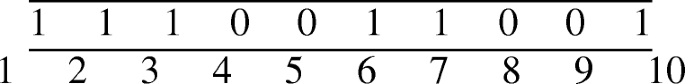

A snapshot of L_opt of size 10 at the BS at the end of step 2

Step 3: :

The BS determines the identification of active VSNs using the position of logic 1 in L_opt. The BS searches the BT to find the records corresponding to the identification of the active VSNs as obtained from L_opt, reads position and orientation from these records to generate FoV of these active VSNs. The BS counts the number of random points in the target area that are inside the FoV of active VSNs as CoV_Randpoints using Eq. 7, uses Eq. 6 to compute the value of Per_CoV using the value of Tot_Randpoints and CoV_Randpoints. Per_CoV should not be less than Init_CoV when Obj_F is equal to Act_VSN_opt. Init_CoV should also be greater than Th_coverage so that WVSN may remain functional. The BS stores Act_VSN_opt as the optimal value of the objective functions Obj_F and Energy$_{Tot\_opt}$ in two separate variables.

Step 4: :

The BS determines the identification of inactive VSNs using the position of logic 0 in L_opt. The BS searches the BT to find the records corresponding to the identification of the inactive VSNs as obtained from L_opt, reads the position from these records and sends sleep messages to these inactive VSNs. The BS also updates these records in the BT by replacing the value of “isVSNActive” Boolean variable from 1 to 0.

4.3 DCC₂

DCC₂ utilizes AGA[12] based single-objective optimization technique to minimize Obj_F subject to connectivity constraint and coverage constraint. AGA is a special category of genetic algorithm (GA) that has characteristics like self-adaptive crossover and mutation operation, scale reproduction etc [12]. AGA adaptively varies the mutation and crossover probability following different conditions of solutions to prevent premature convergence, preserve the solution diversity, to enhance the speed of calculation and the algorithm precision while searching for the optimum value of the objective function. In DCC₂, each solution (also known as a chromosome) belonging to a population of size N_P is of length T_N. The value of Status_v is in the v^th location in the solution. All the solutions in the population are encoded in binary format as the status of each VSN is a binary variable. It is called the genetic representation of a solution. The general format of the genetic representation of a solution is shown in Fig. 5.

Fig. 5

Genetic representation of a solution

Algorithm 1

GA_OPT(N_P, Gen_Max, p^mu, p^cr).

DCC₂ is divided into two parts

Part 1 finds the near-optimal solution and near-optimal value of Obj_F and Part 2 finds shutting off the maximum number of VSNs in the target area.

Part 1: :

To find the near-optimal solution, Procedure GA_OPT() is executed.

Part 2: :

Shutting off the maximum number of VSNs on the target area

Step 2.1: The BS determines the identification of inactive VSNs using the position of logic 0 in L_opt. The BS searches the BT to find the records corresponding to the identification of the inactive VSNs as obtained from L_opt, reads position from these records and sends sleep messages to these inactive VSNs. The BS also updates these records in the BT by replacing the value of the “isVSNActive” Boolean variable from 1 to 0.

4.4 Post duty cycling scenario

A maximum number of VSNs enter into sleep mode after the execution of DCC₁/(DCC₂) by the BS. Now, the BS computes T_N, number of VSNs in sleep mode (say ${\Gamma }_{\max \limits }$) and Act_VSN_opt (=(T_N –${\Gamma }_{\max \limits }$)) from L_opt for the target area. The BS also calculates Per_CoV by Act_VSN_opt in the target area from the BT. In the case of (Per_CoV < Th_coverage ), the BS stops gathering data from WVSN since WVSN is no more operational now. Suppose VSN v is in active mode and (Per_CoV ≥ Th_coverage), the VSN v begins monitoring the target area. Owing to the continuous dissipation of energy, VSN v dies after a certain time. Its energy having been reduced to the value, a little more than zero, the VSN v transmits and routes (utilizing GPSR) dead messages [14] to its neighbors and the BS respectively. The size of the dead message (Size_D) is 17 bits [14]. The BS searches the BT using the id of the VSN v after receiving the dead message from it, updating the values, isVSNActive [14] and isVSNDead [14] to 0 and 1 respectively for VSN v. VSN v₁ (a neighbor VSN of the VSN v say) becomes active when it receives a dead message from the VSN v. These phenomena will happen for all dead VSNs and consequently, the sleeping VSNs belonging to ${\Gamma }_{\max \limits }$ become active. The BS now searches for records of sleeping VSNs (belonging to the set ${\Gamma }_{\max \limits }$) in the BT with the observation of values of “isVSNActive” and “isVSNDead” set as 0 and 0 respectively. VSNs being active now, the BS updates the values of “isVSNActive” and isVSNDead to 1 and 0 respectively.

All the sleeping VSNs (∈ ${\Gamma }_{\max \limits }$) being active, the BS again calculates Per_CoV by ${\Gamma }_{\max \limits }$(=(T_N -Act_VSN_opt)) number of VSNs. The BS will stop collecting data from WVSN at this point if Per_CoV is less than Th_coverage. Otherwise, Act_VSN (∈ Γ_max) will go on monitoring the target area till they die owing to energy deficiency.

5 Qualitative performance

The evaluation of the qualitative performance is carried out with respect to communication overhead (CM_OV), computation overhead (CP_OV), and storage overhead (ST_OV) for the two schemes (PA_1 and PA_2). The existing approach, ET_3 corresponds to EX_3 of [14]. The CM_OV, CP_OV, and ST_OV of APP_5, APP_6, and ET_3 are already evaluated in [14] and are shown in Tables 3 and 4. In the worst case, each VSN in the target area for PA_1 and PA_2 has (T_N-1) number of neighbor VSNs. The overheads are studied in the worst case in the target area.

Table 3 Comparative study of CM_OV and ST_OV Among PA_1, PA_2, APP_5, APP_6 and ET_3 for T_N = 70

Table 4 Comparative study of CM_OV and ST_OV Among PA_1, PA_2, APP_5, APP_6 and ET_3 for T_N = 100

CM_OV: CM_OV of PA_1 and PA_2 is the summation of the communication overhead in the neighbor discovery phase (CM_OV₁), registration phase (CM_OV₂) and duty cycling phase (CM_OV₃).

CM_OV₁: In PA_1 and PA_2 each VSN sends a packet of size Size_Rec_NT bits [14] to its (T_N-1) number of neighbors. Therefore, CM_OV₁ in PA_1 and PA_2 is (Size_Rec_NT*T_N*(T_N-1)) bits

CM_OV₂: In PA_1 and PA_2 each VSN routes a packet of size Size_Rec_NT bits [14] to the BS. So CM_OV₂ in PA_1 and PA_2 is (Size_Rec_NT*T_N) bits

CM_OV₃: In PA_1 and PA_2 the BS routes sleep message of size Size_id bits to (T_N-Act_VSN_min) number of VSNs. A dead message of size Size_D is sent by each VSN to its (T_N-1) number of neighbors and to the BS respectively in PA_1 and PA_2. Hence, CM_OV₃ is (Size_id)*(T_N- Act_VSN_min) + (Size_D)*T_N*(T_N-1)+(Size_D)*(T_N) bits for PA_1 and PA_2

ST_OV: ST_OV of PA_1 and PA_2 is the summation of the storage overhead in the neighbor discovery phase (ST_OV₁), registration phase (ST_OV₂) and duty cycling phase (ST_OV₃).

ST_OV₁: Each VSN stores T_N number of records each of size Size_Rec_NT bits [14] in PA_1 and PA_2. So ST_OV₁ in PA_1 and PA_2 are (Size_Rec_NT*T_N*T_N) bits.

ST_OV₂: In PA_1 and PA_2, the BS stores T_N number of records in the BT. Each record has (Tot_Param+ 2) number of parameters [14] of size (Size_Rec_NT+ 2) bits [14]. So, ST_OV₂ in PA_1 and PA_2 is (Size_Rec_NT+ 2)*T_N bits.

ST_OV₃: The BS stores the optimal solution in L_opt after the execution of DCC₁ in PA_1 and DCC₂ in PA_2. Size_L_opt is T_N bits, i.e., (1/8)*T_N bytes. The BS stores (Act_VSN_opt, Energy$_{Tot\_opt}$) in two separate variables both in PA_1 and PA_2. The data type of the variable which holds the value of Act_VSN_opt is int. The data type of the variable which holds the value of Energy$_{Tot\_opt}$ is float. Therefore, the total size needed to hold Act_VSN_opt and Energy$_{Tot\_opt}$ is (2 + 4) bytes, i.e., 6 bytes. So, ST_OV₃ both in PA_1 and PA_2 are ((1/8)*T_N + 6) bytes.

CP_OV: CP_OV of PA_1 and PA_2 is the summation of the computation overhead in the neighbor discovery phase (CP_OV₁), registration phase (CP_OV₂) and duty cycling phase (CP_OV₃).

CP_OV₁: Each VSN inserts T_N number of records in its neighbor table in the two schemes. In PA_1 and PA_2, each record consists of Tot_Param [14] number of parameters. So, CP_OV₁ in PA_1 and PA_2 is O(Tot_Param*T_N), i.e., O(T_N)

CP_OV₂: The BS inserts T_N number of records in the BT in PA_1 and PA_2. Each record in the BT contains (Tot_Param + 2) number of parameters. So, CP_OV₂ in PA_1 and PA_2 is O((Tot_Param+ 2)*T_N)), i.e., O(T_N)

CP_OV₃: The computation overhead of PA_1 in the duty cycling phase is due to the computation overhead of DCC₁ executed by the BS. DCC₁ employs the ILP-based optimization technique. In this phase, 2$^{T\_N}$ number of possible values to the decision variables (Status₁, Status₂, ...... Status$_{T\_N}$) are assigned in a non-deterministic manner. The computation overhead to check the feasibility of each solution is O(T_N) and to evaluate the value of the objective function for each solution is O(T_N).

The computation overhead of PA_2 in the duty cycling phase is due to the computation overhead of DCC₂ executed by the BS. The computation overhead of AGA utilized by DCC₂ is O(population size * length of each chromosome * number of generations), i.e., O(N_P * T_N * Gen_MAX). The BS stores the near-optimal solution in L_opt with a computation overhead is O(1). The BS computes (Act_VSN_opt and Energy$_{Tot\_opt}$) corresponding to the near-optimal solution in L_opt and inserts them in two separate variables with computation overhead O(T_N).

So, CP_OV₃ in

• PA_1 is 2$^{T\_N}$ x {O(T_N) + O(T_N)}, i.e., O(2$^{T\_N}$ * T_N), i.e., exponential

• PA_2 is O(N_P * T_N * Gen_MAX) + O(1) + O(T_N), i.e., O(N_P * T_N * Gen_MAX) + O(T_N), i.e., polynomial in nature.

  Therefore, CP_OV in

• PA_1 is O(T_N) + O(T_N) + O(2$^{T\_N}$ * T_N), i.e., O(T_N x 2$^{T\_N}$), i.e., exponential in nature.

• PA_2 is O(T_N) + O(T_N) + O(N_P * T_N * Gen_MAX) + O(T_N), i.e., O(T_N) + O(N_P * T_N * Gen_MAX), i.e., polynomial in nature.

• APP_5 [14] and APP_6 [14] is O(T_N⁶) [14]

• ET_3 is O(T_N²) [14]

CP_OV is the highest in PA_1 (exponential) and the lowest in ET_3. CP_OV of APP_5 and APP_6 are the same. CP_OV of ET_3 is lesser than that of APP_5, APP_6. CP_OV of PA_2 cannot be compared with PA_1, APP_5, APP_6, and ET_3 as CP_OV of PA_2 depends on two other variables, Gen_MAX and N_P apart from T_N unlike CP_OV of the rest of the approaches.

CM_OV and ST_OV for the five schemes are calculated and shown in Tables 3 and 4 respectively when T_N is 70 and 100.

It is observed from Tables 3 and 4 that CM_OV is the least and the same for PA_1 and PA_2. CM_OV is the highest in ET_3. CM_OV is less in APP_5 and APP_6 than in ET_3. It is also observed from Tables 3 and 4 that ST_OV is the least in PA_1 and PA_2, the highest in APP_5 and APP_6, and less in ET_3 than in APP_5 and APP_6.

6 Quantitative performance

Both PA_1 and PA_2 are simulated using OMNET+ + Castalia simulator [31]. WVSN−v4 framework [32] which supports the modeling of video sensor coverage contains a simulation model of WVSN. A particular VSN possessing a larger processing capability is supposed to be the BS both in PA_1 and PA_2. The BS utilizes pulp [30] and pymoo [33] (both are python-based packages) to get an optimal solution and a near-optimal solution respectively in the duty cycling phase. Pymoo is a python-based package for solving the problem of optimization utilizing different stochastic methods like GA, NSGA-II, PSO, etc. The performance of PA_1 and PA_2 is compared with APP_5 and APP_6 in [14]. Hence, the basic simulation environment, simulation environment for energy consumption, tunable MAC parameters, and GPSR protocol parameters as in [14] are summarized in Tables 5¹, 6, 7, and 8 respectively. Tables 5, 6, 7, and 8 correspond to Tables 5, 6, 7, and 8 in [14] respectively. Table 9 summarizes the parameters used in DCC₂.

Table 5 The basic experimental parameters for PA_1 & PA_2

Table 6 The experimental parameters for energy consumption in PA_1 and PA_2

Table 7 Tunable MAC parameters for PA_1 and PA_2

Table 8 GPSR protocol parameters for PA_1 and PA_2

Table 9 Parameters used in DCC₂ of PA_2

6.1 Simulation metric

The quantitative performance of PA_1 and PA_2 is studied based on Act_VSN, E_Tot (in Joule), E_Res (in Joule), Per_CoV (in percentage), network lifetime (in seconds) and R_T (in seconds) in the target area. R_T is the execution time (in seconds) of PA_1, PA_2 excluding the execution time of the neighbor discovery phase and registration phase.

The quantitative performance of PA_2 is also studied based on Act_VSN for studying the convergence of GA_ OPT to the optimum value of Act_VSN, i.e., Act_VSN_opt.

With the increase in the total number of deployed VSNs in the target area (node density) Act_VSN increases and as a result of which E_Tot, Per_CoV, E_Res and network lifetime also increase. Therefore, the variation of Act_VSN, E_Tot, E_Res, Per_CoV and network lifetime is studied with the variation of the node density during simulation. With the increase in node density, R_T increases as a result of which network lifetime also increases. Therefore, the variation of R_T is studied with the variation of the node density during simulation. The increase in the total number of function evaluations (Function Evaluation) defined as the product of population size and the number of generations in GA_OPT decreases Act_VSN if GA_OPT converges to the optimum value of Act_VSN, i.e., Act_VSN_opt. Therefore, the variation of Act_VSN is examined by varying Function Evaluation during simulation.

6.2 Simulation results and performance evaluation

Five simulation experiments are conducted to compare the performance of PA_1 and PA_2 with APP_5, APP_6, ET_3 and Init_Ran. The sixth simulation experiment is conducted to compare the performance of PA_1 and PA_2 with APP_5, APP_6 and ET_3. The seventh simulation experiment is also conducted during the simulation of PA_2 for studying the convergence of GA_OPT to Act_VSN_opt. All the simulation experiments except the fifth, sixth and seventh simulation experiments have been conducted for the duration (0–700) s. The fifth simulation experiment is conducted for (0–1500) s.

6.2.1 Act_VSN versus node density

The first simulation experiment is conducted for observing the variation of Act_VSN with node density. The plot of Act_VSN vs. node density for Init_Ran, PA_1, PA_2, APP_5, APP_6, and ET_3 is shown in Fig. 6.

Fig. 6

Act_VSN vs node density

Observation from Fig. 6

Act_VSN increases with node density for all the six schemes (Init_Ran, PA_1, PA_2, APP_5, APP_6, ET_3), which is quite obvious. Act_VSN is the highest for Init_Ran and the least for PA_1, less in PA_2 than in APP_5, APP_6, and ET_3, less in APP_6 than in APP_5, ET_3, less in APP_5 than in ET_3 (for node density > 100).

6.2.2 E_Tot versus node density

The second simulation experiment is conducted for observing the variation of E_Tot with node density. The plot of E_Tot vs. node density for Init_Ran, PA_1, PA_2, APP_5, APP_6 and ET_3 is shown in Fig. 7.

Fig. 7

E_Tot vs node density

Observation from Fig. 7

E_Tot increases with node density for all the six schemes (Init_Ran, PA_1, PA_2, APP_5, APP_6, ET_3). E_Tot is the largest for Init_Ran and the minimum for PA_1, less in PA_2 than in APP_5, APP_6 and ET_3, less in APP_6 than in APP_5, ET_3, less in APP_5 than in ET_3 (for node density > 100). This result is obvious from the nature of graphs shown in Fig. 6 which plots Act_VSN vs. node density since E_Tot is directly proportional to Act_VSN according to Eq. 1.

6.2.3 E_Res versus node density

The third simulation experiment is conducted for observing the variation of E_Res with node density. The plot of E_Res vs. node density for Init_Ran, PA_1, PA_2, APP_5, APP_6, and ET_3 is shown in Fig. 8.

Fig. 8

E_Res vs node density

Observation from Fig. 8

E_Res increases with node density for all the six schemes (Init_Ran, PA_1, PA_2, APP_5, APP_6, ET_3). E_Res is the least for Init_Ran and the largest for PA_1, greater in PA_2 than in APP_5, APP_6 and ET_3, greater in APP_6 than in APP_5, ET_3, greater in APP_5 than in ET_3 (for node density > 100). This result is obvious from the nature of the graphs shown in Fig. 7 which plots E_Tot vs. node density since E_Res is equal to (Total Initial Energy of VSNs − E_Tot)

6.2.4 Per_CoV versus node density

The fourth simulation experiment is conducted for observing the variation of Per_CoV with node density. The plot of Per_CoV vs. node density for Init_Ran, PA_1, PA_2, APP_5, APP_6 and ET_3 is shown in Fig. 9.

Fig. 9

Per_CoV vs node density

Observation from Fig. 9

Per_CoV increases with node density for all the six schemes (Init_Ran, PA_1, PA_2, APP_5, APP_6, ET_3). Per_CoV is the largest for Init_Ran, PA_1, PA_2 and the lowest for APP_6, less in APP_5 than ET_3 (for node density > 100). The nature of graphs in Fig. 6 explains the nature of graphs in Fig. 9.

6.2.5 Network lifetime versus node density

The fifth simulation experiment is conducted for observing the variation of network lifetime with node density. The plot of network lifetime vs. node density for Init_Ran, PA_1, PA_2, APP_5, APP_6 and ET_3 is shown in Fig. 10.

Fig. 10

Network lifetime vs node density

Observation from Fig. 10

Network lifetime is the least in Init_Ran and ET_3 (770 s) and the highest in PA_1 and PA_2 (1500 s) for all node density. It is lesser in APP_6 than in PA_1 and PA_2 for the node density less than equal to 80. It is lesser in APP_5 than in PA_1, PA_2 and APP_6 for all node densities except node densities 120 and 150. The nature of graphs in Fig. 8 explains the nature of graphs in Fig. 10.

6.2.6 Comparison among PA_1, PA_2, APP_5, APP_6 and ET_3 with respect to R_T

The sixth simulation experiment is conducted for observing the variation of R_T with node density. Tables 10 and 11 describe R_T of PA_1, PA_2, APP_5, APP_6 and ET_3. R_T for these approaches in ascending order for all objective functions considered here is described as follows: R_T of ET_3 < R_T of APP_5 < R_T of APP_6 < R_T of PA_1 << R_T of PA_2 << R_T of PA_1(Theoretical). It is small for APP_5, APP_6, and ET_3, as they are greedy approaches, and the largest for PA_1(Theoretical)(Theoretical value of R_T of PA_1) as the computational complexity of ILP is exponential in nature theoretically (as discussed in CP_OV₃ of Section 5). It is small for PA_1 as it uses CBC solver to solve ILP. Modern solvers like CBC can solve single-objective ILP of large problem size within 4 seconds [34]. R_T value is moderate for PA_2 as it uses AGA heuristic. Tables 10 and 11 clearly show that with the increase in the number of generations (gen) in PA_2, R_T increases which is obvious. It is to be noted that, a small network of 3D VSNs (16–18) VSNs on a 25m X 25 m target area) is created to measure R_T of all the approaches as the computational complexity of PA_1(Theoretical) is exponential.

Table 10 R_T (in s) of PA_1, PA_2, APP_5, APP_6 and ET_3 for Tot_VSN= 16

Table 11 R_T (in s) of PA_1, PA_2, APP_5, APP_6 and ET_3 for Tot_VSN= 18

6.2.7 Act_VSN versus function evaluation

The seventh simulation experiment is conducted for observing the variation of Act_VSN with Function Evaluation in PA_2. The plot of Act_VSN versus Function Evaluation for PA_2 is shown in Figs. 11 and 12 when node density equals 70 and 80 respectively.

Fig. 11

Act_VSN vs function evaluation (Node Density= 70) for PA_2

Fig. 12

Act_VSN vs function evaluation (Node Density= 80) for PA_2

Observation from Figs. 11 and 12

Act_VSN decreases with Function Evaluation. It is also observed from Figs. 11 and 12 that Act_VSN becomes almost parallel to the Function Evaluation axis when Function Evaluation is greater than 1500 and 4500 respectively. It means Act_VSN has already reached its optimal value (Act_VSN_opt) at Function Evaluation greater than 1500 (or Gen_Max > 15) and greater than 4500 (or Gen_Max > 45) in Figs. 11 and 12 respectively.

6.3 Experimental analysis

In PA_1, PA_2, APP_5, and APP_6 the collision among messages and consequently loss in messages is reduced by tunable MAC protocol which utilizes CSMA/CA for reducing the message collision. As a result, the BS receives all the messages from VSNs in the registration phase. The BS in PA_1, PA_2/(APP_5, APP_6) sends a sleep message again using tunable MAC protocol for turning off T_N-Act_VSN_opt number of/(a set of) VSNs. This results in the minimization of Act_VSN as observed in Fig. 6 and minimization of E_Tot as observed in Fig. 7 which leads to the maximization of E_Res (as observed in Fig. 8) and in turn network lifetime (as observed from Fig. 10) both in PA_1 and PA_2. This also results in the reduction in Act_VSN, E_Tot, Per_CoV and an increase in E_Res, network lifetime in the case of APP_5 (for node density > 100) and APP_6 in comparison to ET_3 as observed from Figs. 6, 7, 9, 8 and 10 respectively. The four BSs operate simultaneously in APP_6. Hence, the BS in APP_6 receives most of the request messages from the VSNs in the target area. This reduces Act_VSN, E_Tot, Per_CoV and enhances E_Res, and network lifetime more in APP_6 than in APP_5 and ET_3. The minimization of Act_VSN both in PA_1 and PA_2 (Fig. 6) results in no reduction of Per_CoV from Init_CoV as observed in Fig. 9. Therefore, Per_CoV is the highest in PA_1 and PA_2 and it is the same as Init_Ran.

No message-passing takes place in the duty cycling phase of PA_1 and PA_2. Therefore, CM_OV of PA_1 and PA_2 is the least as observed in Tables 3 and 4. Act_VSN_opt in PA_1 is optimal (minimum) and Act_VSN_opt in PA_2 is near-optimal. Therefore, Act_VSN_opt and Energy$_{Tot\_opt}$ in PA_1 are lesser than Act_VSN_opt and Energy$_{Tot\_opt}$ in PA_2 as observed from Figs. 6 and 7 respectively. E_Res in PA_1 is greater than E_Res in PA_2 for the same reason as observed from Fig. 8. PA_2 being based on AGA produces very good results in terms of minimizing Act_VSN and E_Tot, and maximizing E_Res and network lifetime while maintaining Per_CoV equal to Init_CoV compared to that obtained by using APP_5, APP_6 and ET_3 (as observed from Figs. 6, 7, 8, 9 and 10 (respectively).

The group leader [13] in the grid sends a sleep message to the two VSNs belonging to the q^th grid having the highest and second-highest weight respectively in ET_3. The VSNs get the sleep message from the corresponding group leader and broadcast the SAM message [13] to their corresponding neighbors. There is a collision between the sleep messages and the SAM message although sleep messages do not collide with each other across the grids in the target area. This results in a loss of sleep message. The loss of sleep message owing to collision enhances with the enhancement of deployed VSNs in the target area. A huge number of VSNs having the highest or second-highest weight in several grids do not receive sleep messages from their corresponding group leader and consequently, those VSNs remain active although they fulfill the condition of redundant coverage [13, 14]. This enhances Act_VSN (Fig. 6), E_Tot (Fig. 7) and Per_CoV (Fig. 9) and decreases E_Res (Fig. 8) and network lifetime (Fig. 10) in ET_3 compared to APP_5 (for node density > 100).

6.4 Summary of major observation

It is observed that APP_6 produces a better result than that of (APP_5, APP_6, and ET_3) with regard to E_Tot. ET_3 shows the best results among these three state-of-the-art works with regard to Per_CoV. Act_VSN is lesser in PA_1 compared to PA_2. PA_1 and PA_2 are able to reduce E_Tot by 40.85% and 33.34% respectively from the existing best approach APP_6 (with respect to E_Tot) for 150 deployed VSNs over the target area. With the reduction in Act_VSN, E_Tot also decreases but at the expense of reduced Per_CoV in APP_5, APP_6, and ET_3. But the reduction in Act_VSN does not cause a reduction in Per_CoV in PA_1 and PA_2. For the same node density, both PA_1 and PA_2 gain a little amount of Per_CoV (i.e., 0.94%) than the existing better approach ET_3 (in terms of Per_CoV). Both PA_1 and PA_2 have the same CM_OV. Both of them show better results by 0.32%/(4.25%) from (APP_5 & APP_6)/(ET_3) in terms of CM_OV for 100 deployed VSNs on the same target area. Finally, PA_1 reveals its superiority concerning reduced E_Tot (11.26%) over that of PA_2 without losing Per_CoV for 150 deployed VSNs.

7 Conclusions

In this paper, two advanced approaches, PA_1 and PA_2 have been proposed to minimize the number of active 3D video sensor nodes monitoring the 2D target area without losing area coverage and ensuring network connectivity in the target area with randomly deployed VSNs. The total energy consumption by the video sensor nodes being proportional to the number of active video sensor nodes, PA_1 and PA_2 is designed for minimizing energy consumption. PA_1 produces the optimal value of energy consumption, while PA_2 produces a near-optimal value of energy consumption, subject to coverage and connectivity constraints. APP_5, APP_6, and ET_3 are the existing state-of-the-art approaches with which PA_1 and PA_2 are compared both with regard to energy consumption and area coverage. It is observed that both PA_1 and PA_2 produce much better results while minimizing energy consumption and also maintaining the initial coverage compared to APP_5, APP_6, and ET_3.

A new approach can be developed in the future to address the above-mentioned conflicting issues in the presence of heterogeneous 3D video sensor nodes where all video sensor nodes will have different communication and sensing ranges.

References

Bairagi K, Mitra S, Bhattacharya U (2020) Coverage aware dynamic scheduling strategies for wireless video sensor nodes to reduce energy consumption. In: 11th International conference on computing, communication and networking technologies (ICCCNT). IEEE, pp 1–7. https://doi.org/10.1109/ICCCNT49239.2020.9225516
Bairagi K, Bhattacharya U (2019) Resource constrained coverage model of a video sensor node to reduce energy consumption. In: International conference on electrical, computer and communication technologies (ICECCT), Coimbatore, India. IEEE, pp 1–7. https://doi.org/10.1109/ICECCT.2019.8869026
Bendimerad N, Kechar B (2015) Rotational wireless video sensor networks with obstacle avoidance capability for improving disaster area coverage. J Inform Process Syst 11 (4):509–527. https://doi.org/10.3745/JIPS.03.0034
Bendimerad N, Kechar B (2014) Coverage enhancement with rotatable sensors in Wireless Video Sensor Networks for post-disaster management. In: 1st International conference on information and communication technologies for disaster management (ICT-DM), Algiers. IEEE, pp. 1–7. https://doi.org/10.1109/ICT-DM.2014.6918584
Salim A, Osamy W, Khedr A (2018) Effective scheduling strategy in wireless multimedia sensor networks for critical surveillance applications. Appl Math Inform Sci 12(1):101–111. https://doi.org/10.18576/amis/120109
Makhoul A, Abdallah, Pham C (2009) Dynamic scheduling of cover-sets in randomly deployed wireless video sensor networks for surveillance applications. In: 2nd IFIP wireless days. IEEE, pp 1–6. https://doi.org/10.1109/WD.2009.5449700
Ukani V, Patel K, Zaveri T (2015) In: IEEE Region 10 Symposium, Ahmedabad. IEEE, pp 37–40. https://doi.org/10.1109/TENSYMP.2015.23
Benzerbadj A, Kechar B (2013) Redundancy and criticality based scheduling in wireless video sensor networks for monitoring critical areas. Procedia computer science (ELSEVIER) 21(2013):234–241. https://doi.org/10.1016/j.procs.2013.09.031
Ukani V, Patel K, Zaveri T (2015) A realistic coverage model with backup set computation for wireless video sensor network. Nirma Univ J Eng Technol 4(1):1–5
Integer programming. Retrieved June 16, 2021 from. https://en.wikipedia.org/wiki/Integer_programming
Mehboob U, Qadir J, Ali S et al (2016) Genetic algorithms in wireless networking: techniques, applications, and issues. Soft Comput 20(2016):2467–2501. https://doi.org/10.1007/s00500-016-2070-9
Tian J, Gao M, Ge G (2016) Wireless sensor network node optimal coverage based on improved genetic algorithm and binary ant colony algorithm. J Wireless Com Network 2016(1):104. https://doi.org/10.1186/s13638-016-0605-5
Zhang K, Chen J, Shen C, Chen Y, Long K, Aslam BU (2019) Node Scheduling Algorithm Based on Grid for Wireless Sensor Networks. In: 19th International conference on communication technology (ICCT). IEEE, pp 987–990. https://doi.org/10.1109/ICCT46805.2019.8947095
Bairagi K, Mitra S, Bhattacharya U (2021) Coverage aware scheduling strategies for 3D wireless video sensor nodes to enhance network lifetime. IEEE Access 9:124176–124199. https://doi.org/10.1109/ACCESS.2021.3110271
Wang P, Dai R, Akyildiz If (2013) A differential coding-based scheduling framework for wireless multimedia sensor networks. IEEE Trans Multimedia 15(3):684–697. https://doi.org/10.1109/TMM.2012.2236304
Yu C, Sharma G (2010) Camera scheduling and energy allocation for lifetime maximization in user-centric visual sensor networks. IEEE Trans Image Process 19(8):2042–2055. https://doi.org/10.1109/TIP.2010.2046794
Jamshed MA, Khan MF, Rafique K, Khan MI, Faheem K, Shah SM, Rahim A (2015) An energy efficient priority based wireless multimedia sensor node dynamic scheduler. 12th International Conference on High-capacity Optical Networks and Enabling/Emerging Technologies (HONET), Islamabad. IEEE, pp 1–4. https://doi.org/10.1109/HONET.2015.7395435
Bhosale VD, Satao RA (2015) Lifetime maximization in mobile visual sensor network by priority assignment. International Conference on Control, Instrumentation, Communication and Computational Technologies (ICCICCT), Kumaracoil. IEEE, pp 695–698. https://doi.org/10.1109/ICCICCT.2015.7475368
Khursheed K, Imran M, O′Nils M, Lawal N (2010) Exploration of local and central processing for a wireless camera-based sensor node. In: ICSES international conference on signals and electronic circuits, Gliwice. IEEE, pp 147–150
Jun-Woo Ahn, Tai-Woo Chang, Sung-Hee Lee, Won Seo Yong (2016) Two-phase algorithm for optimal camera placement. Scientific Programming (Hindawi), vol. 2016. ArticleID 4801784:16. https://doi.org/10.1155/2016/4801784
Fu Y, Zhou J, Deng L (2014) Surveillance of a 2D Plane Area with 3D deployed cameras. Sensors 14(2):1988–2011. https://doi.org/10.3390/s140201988
Xu Y, Jiao W, Tian M (2020) Energy-efficient connected-coverage scheme in wireless sensor networks. Sensors 20(21):6127. https://doi.org/10.3390/s2021612
Saadaldeen Razan SM, Ahmed Yousif EE, Osman Abdalla A (2020) An Approach to Efficient Data Redundancy Reduction While Preserving the Full Coverage in a WSN. IRJET 7(7):780–790
Qin N, Chen J (2018) An area coverage algorithm for wireless sensor networks based on differential evolution. Int J Distrib Sens Netw 14(8):1–11. https://doi.org/10.1177/1550147718796734
Shanti DL, Prasanna K (2021) Computational Intelligence based WSN lifetime extension with maximizing the disjoint Set K-Cover. Turkish J Comput Math Educ 12(11):3832–3849
Dong L, Tao H, Doherty W, Young M (2015) A sleep scheduling mechanism with PSO collaborative evolution for wireless sensor networks. Int J Distrib Sens Netw 11(3):1–12. https://doi.org/10.1155/2015/517250
Zhou J, Xu M, Lu Yi, Yang R (2020) Research on coverage control algorithm based on wireless sensor network. MATEC Web Conf. EDP Sciences, France 309:03003. https://doi.org/10.1051/matecconf/202030903003
Karp B, Kung HT (2000) GPSR: greedy perimeter stateless routing for wireless networks. In: Proceedings of the 6th annual international conference on Mobile computing and networking (MobiCom ’00), pp 243–254
Philips TK, Panwar SS, Tantawi AN (1989) Connectivity properties of a packet radio network model. IEEE Trans Inf Theory 35(5):1044–1047
Mitchell S, O’Sullivan M, Dunning I (2011) PuLP: a linear programming toolkit for python. The University of Auckland, Auckland, New Zealand. Retrieved Jun. 16, 2021, from. http://www.optimization-online.org/DB_FILE/2011/09/3178.pdf
Pham C (2015) A video sensor simulation model with OMNET++, Castalia Extension. Retrieved Sep. 25, 2016, from. http://cpham.perso.univ-pau.fr/WSN-MODEL/wvsn-castalia.html
Pham C (2011) A video sensor simulation model with OMNET++. Retrieved Sep. 25, 2016, from. http://cpham.perso.univ-pau.fr/WSN-MODEL/wvsn.html
Blank J, Deb K (2020) Pymoo: multi-objective optimization in python. IEEE Access 8:8949–89509. https://doi.org/10.1109/ACCESS.2020.2990567
Veerapen N, Ochoa G, Harman M, Burke E (2015) An integer linear programming approach to the single and bi-objective next release problem. Inf Softw Technol 65(2015):1–13. https://doi.org/10.1016/j.infsof.2015.03.008
Author information
Authors and Affiliations
Corresponding author
Ethics declarations
Competing interests
The authors declare no competing interests.
Additional information
Availability of data
The data underlying this article will be shared on reasonable request to the corresponding author.
Publisher’s note
Springer Nature remains neutral with regard to jurisdictional claims in published maps and institutional affiliations.
Rights and permissions
Springer Nature or its licensor (e.g. a society or other partner) holds exclusive rights to this article under a publishing agreement with the author(s) or other rightsholder(s); author self-archiving of the accepted manuscript version of this article is solely governed by the terms of such publishing agreement and applicable law.
About this article
Cite this article
Bairagi, K., Mitra, S. & Bhattacharya, U. Efficient approaches to optimize energy consumption in 3D wireless video sensor network under the coverage and connectivity constraints. Ann. Telecommun. 78, 329–346 (2023). https://doi.org/10.1007/s12243-023-00947-w
Received:
Accepted:
Published:
Issue Date:
DOI: https://doi.org/10.1007/s12243-023-00947-w