Differential uniformity and linearity of S-boxes by multiplicative complexity

Abstract

A cryptographic primitive with low multiplicative complexity (MC) makes various applications efficient, but it may lead to cryptographic vulnerabilities. To find a trade-off between cryptographic resistance and MC, we propose a new tool called A-box, which is constructed using AND gates. In this paper, we prove several important properties of A-boxes, which provide the theoretical lower bounds of differential uniformity and linearity of corresponding S-boxes by MC. Specifically, we show that the differential uniformity (resp. linearity) of an (n, m)-bit S-box is at least 2^n−l, where its MC is $\lfloor \frac {n-1}{2}\rfloor +l$ (resp. m − 1 + l). Furthermore, we develop an algorithm to find S-boxes with differential uniformity equal to the bounds with respect to their MC. We improve the algorithm previously proposed by Zajac and Jókay (Cryptogr. Commun. 6(3), 255–277, 2014), which is applicable only to S-boxes of size lower than 5 bits, whereas ours can run on larger-sized S-boxes. We found a bijective (8,8)-bit S-box with differential uniformity 16, linearity 128, and 8 nonlinear gates: this has better cryptographic security than the SKINNY S-box with differential uniformity 64, linearity 128, and 8 nonlinear gates. We believe that our results provide a better understanding of the relationship between cryptographic resistance and MC of S-boxes.

1 Introduction

Reducing the number of nonlinear gates when implementing cryptographic primitives, especially using block ciphers, is an important concern in various fields [2, 34] such as post quantum zero-knowledge (PQZK) proofs, multi-party computation (MPC) protocols [23], fully homomorphic encryption (FHE), and side-channel attacks (SCAs) [29]. In PQZK proofs based on “MPC-in-the-head,” the signature size increases proportionally to the number of nonlinear gates used in the underlying block cipher [18]. The computational complexity in the MPC protocol based on Yao’s garbled circuit [32, 35] using the free-XOR technique depends on the number of nonlinear gates [30]. For FHE, an AND gate in the underlying block cipher is more expensive than an XOR gate and may generate noise during calculations [26]. Furthermore, the smaller the number of nonlinear gates required to implement the block cipher, the more efficient the SCA countermeasure technique that can be implemented. This is because the cost of Boolean masking increases sharply when it is applied to nonlinear gates rather than linear ones. Therefore, cryptographic primitives that can be implemented using a small number of nonlinear gates have many advantages in various applications.

The multiplicative complexity (MC) of a vectorial Boolean function is the minimal number of AND gates needed to implement it over the basis {AND, XOR, NOT} (called an XOR-AND circuit [13]). As stated above, obtaining a primitive with low MC is important for performance; however, such a primitive may have potential cryptographic vulnerabilities. For example, block ciphers based on an S-box with low MC may be vulnerable to cryptanalysis [16].

In this paper, we discuss security against differential and linear cryptanalyses (DC and LC, respectively) in an S-box based on its MC [6, 31]. As DC and LC are the most influential techniques among block cipher cryptanalyses [27], the differential uniformity and linearity of an S-box are considered the most important cryptographic properties. For an efficient and secure cryptographic primitive design, it is essential to clarify the trade-off between the MC and differential uniformity/linearity of an S-box.

The lower bounds of differential uniformity and linearity independent of MC have been revealed. While the differential uniformity has an obvious lower bound [5], there are several bounds of linearity: the covering radius bound, Sidelnikov–Chabaud–Vaudenay’s bound [17], and three types of linearity bounds in [16]. Zajac and Jókay investigated the MC of all the affine classes of bijective (4,4)-bit S-boxes [37]. Their investigation used an expansion-compression method to accurately calculate the MC of S-boxes. This leads to the following two facts about bijective (4, 4)-bit S-boxes.

• A bijective (4,4)-bit S-box with optimal differential uniformity 4 has MC at least 4.

• A bijective (4,4)-bit S-box with optimal linearity 8 has MC at least 4.

Božilov et al. investigated the MC of all the affine classes of quadratic (5, 5)-bit S-boxes [14]. There are many open issues for the existence of S-boxes, such as (5, 5)-bit S-boxes with MC 6 and differential uniformity 2 (this study shows that there is no such (5, 5)-bit S-box, which will be explained below). In [10], Boyar and Find found that the number of AND gates, linearity, and the length of the shortest linear code are related. The bounds they found were proved in the ΣπΣ circuit, which consists of sequential XOR, AND, and XOR layers.

Contributions

In this paper, we present a new cryptographic tool called A-box, motivated by the work of Zajac and Jókay [37]. While their expansion function consists of AND and identity parts, we restrict it to only the AND part to define the A-box. Specifically, an S-box can be divided into an A-box (as a nonlinear function) and linear functions. We used several properties of A-boxes to prove the theoretical lower bounds of differential uniformity and linearity of the corresponding S-boxes by MC.

We show that the differential uniformity (resp. linearity) of an (n, m)-bit S-box is at least 2^n−l, where its MC is $\lfloor \frac {n-1}{2}\rfloor +l$ (resp. m − 1 + l). Furthermore, we develop an algorithm to search for A-boxes with differential uniformity equal to our bounds with respect to their MC. Those A-boxes lead to S-boxes with the same differential uniformity as theirs. Table 1 presents the lowest differential uniformity we found, within (n, n)-bit S-boxes with MC k where 3 ≤ n ≤ 8 and 1 ≤ k ≤ 7. Our investigation reveals the following properties:

• A (5, 5)-bit S-box with differential uniformity 2 has MC at least 7.

• A (6,6)-bit S-box with differential uniformity 4 has MC at least 7.

• An (8,8)-bit S-box with differential uniformity 32 has MC at least 7.

Compared to differential uniformity, a relatively large MC is required to reduce linearity. The new S-boxes constructed by our method are compared with existing ones in Table 2. Either they have better differential uniformity or linearity than those of existing S-boxes with respect to the same nonlinear gates or less, or they achieve our lower bounds of both differential uniformity and linearity with respect to MC which is the same as implemented nonlinear gates. The detailed implementation codes are provided in Appendix A.

Table 1 Differential uniformity of (n, n)-bit S-boxes found by our experiments

Table 2 Comparision of (n, n)-bit S-boxes*

Organization

The remainder of this paper is organized as follows. In Section 2, we introduce the expansion-compression method of [37], based on which we define the A-box, and we observe several properties of A-boxes. In Section 3, we use them to prove the theoretical lower bounds of the differential uniformity and linearity of S-boxes by MC. In Section 4, we present an S-box search process in terms of MC and low differential uniformity. We conclude this paper in Section 5.

Preliminary

The following notations and definitions are used throughout this paper.

Table 3

For the convenience of notation, an n-dimensional vector is considered to be a column-matrix when performing matrix multiplication. Therefore, it is defined as follows.

Any linear function can be expressed as the multiplication of a matrix. We indicate the matrix related to the linear function in the subscript of $\mathcal {T}$. For example, the matrix expression of the linear function is an m × n matrix M and we denote for . The dot product of and is denoted by , and its matrix expression is . I_n is the n × n identity matrix. The k LSBs and k MSBs of are expressed as and , respectively. 0⁽ⁿ⁾ is the zero vector of , and 0^(n×m) is the zero matrix of size n × m.

2 A-box and its equivalence classes

2.1 Definition of A-box

Consider an XOR-AND circuit of an S-box. The AND gates on the circuit are made as per the following rule. The inputs of the i^th AND gate are calculated as the linear combinations of three types of bits: the inputs of the S-box, the outputs of the previous i − 1 AND gates, and the constant 1. In addition, the outputs of the circuit are calculated as the linear combinations of three types of bits: the inputs of the circuit, the outputs of the sufficient number of AND gates, and the constant 1. In particular, an S-box with 0↦0 can be constructed with a circuit without using NOT gates. Zajac and Jókay constructed an XOR-AND circuit of such an S-box as the expansion–compression method for expansion function and compression function [37]. As the expansion function is helpful for understanding the concept of the A-box, we explain it first.

For two vectors and an input , the expansion function E_i is defined as follows.

That is, E_i is a function that concatenates the output of one AND gate to the MSB of the input . The for j ∈{0, 1} means a linear combination of input bits. Zajac and Jókay constructed the following function with by composing k expansion functions from E_n to E_n+k− 1.

$$ E_{n+k-1}\circ E_{n+k-2}\circ\cdots\circ E_{n}. $$

(1)

This function (1) describes a circuit using k AND gates. By setting and of each E_n+i, the linear combination of the inputs of each i^th AND gate will be determined. We define as a partner vector and the 2k-tuple that consists of all in order as a partner tuple. By applying a linear function (which is called the compression function in [37]) to function (1), we obtain the following function with ,

$$ \mathcal{T}_{C}\circ E_{n+k-1}\circ E_{n+k-2}\circ\cdots\circ E_{n}. $$

(2)

By Lemma 6 of [37], function (2) expresses any (n, m)-bit S-box with 0↦0. In this method, a circuit with k = C_∧(S) always exists. By XORing function (2) with a constant , we obtain an (n, m)-bit S-box expression with no necessary conditions.

(3)

The output of function (1) consists of a k-bit (called the AND part) and n-bit (called the identity part); the latter n-bit represents the original input. The AND part becomes a type of (n, k)-bit S-box, which we define as an A-box (refer to Fig. 2). Naturally, the MC of an (n, k)-bit A-box is less than or equal to k. To avoid any confusing context, we denote an S-box as S and the corresponding A-box as S_A. The mathematical definition of the A-box is given in Definition 1.

Definition 1

Let and be the input and output, respectively, of an (n, k)-bit S-box S_A. For 2k vectors that satisfy the following inductive properties, S_A is called an (n,k)-bit A-box.

• .

• For 1 ≤ i < k, .

For an (n, k)-bit A-box S_A, and are called i^th partner vectors for all i, and is called the partner tuple of S_A.

A-boxes can be taken from existing S-boxes. For example, Fig. 1 shows an A-box construction taken from the GIFT S-box.

Fig. 1

Process of obtaining an A-box from the implementation of GIFT S-box

We often write the ANF of an A-box S_A as (f_k− 1, ⋯ , f₀). The ANF function f_i satisfies c_∧(f_i) ≤ i + 1. We also denote the components of the i^th partner vectors as follows.

Note that an A-box can have multiple partner tuples. For example, the output of the i^th AND gate of the A-box is invariant even though and are swapped.

2.2 Equivalence classes

For an S-box S and three affine functions A, B, and C, (B ∘ S ∘ A) ⊕ C is called an extended affine transformation (EA transformation). Let $S^{\prime }=(B\circ S\circ A)\oplus C$; then, S is the extended affine equivalent (EA equivalent) to $S^{\prime }$. Furthermore, the set of all S-boxes that are EA equivalent to S is called the extended affine equivalence class (EA class) of S [15]. Similarly, linear equivalence is defined by $S^{\prime }=B\circ S\circ A$ for two linear functions A and B. It is known that MC, differential uniformity, and linearity are invariant under EA transformation [15, 36].

Consider an (n, m)-bit S-box S. By using the form (3), S is given as

(4)

for an (n, k)-bit A-box S_A. As $\mathcal {T}_{C}$ is a linear function, we can decompose into two linear functions, i.e., and . Accordingly, function (4) is transformed as follows.

The matrix $N^{\prime }$ can be decomposed by matrix multiplication of the m × k matrix M in reduced row echelon form (RREF) and the invertible m × m matrix D. Now, we obtain

(5)

This is depicted in Fig. 2. Note that in this figure each rectangle box located to the right of the partner vectors is a linear operator that generates two inputs of the AND gate. Specifically, for the i^th AND gate, the corresponding rectangle box computes the two inputs and .

Fig. 2

Input and output of an (n, m)-bit S-box and an (n, k)-bit A-box

As and are affine functions, S and $\mathcal {T}_{M} \circ S_{A}$ are EA equivalent. Therefore, the following theorem holds.

Theorem 1

For any (n, m)-bit S-box S and k ≥ c_∧(S), there exist an m × k matrix M in RREF and an (n, k)-bit A-box S_A such that $\mathcal {T}_{M} \circ S_{A}$ is EA equivalent to S. If k = c_∧(S), S_A is called suitable for S.

Next, we consider the linear equivalence of an A-box. Let L and $L^{\prime }$ be linear functions on and , respectively. Then, $\mathcal {T}_{L^{\prime }}\circ S_{A} \circ \mathcal {T}_{L}$ is linear equivalent to S_A. Recall that our ultimate goal is to get the S-box, not the A-box. By substituting S_A for $\mathcal {T}_{L^{\prime }}\circ S_{A} \circ \mathcal {T}_{L}$, the $\mathcal {T}_{D}\circ \mathcal {T}_{M}\circ S_{A}$ in (5) is changed to

$$ \begin{array}{@{}rcl@{}} \mathcal{T}_{D}\circ\mathcal{T}_{M}\circ \mathcal{T}_{L^{\prime}}\circ S_{A}\circ \mathcal{T}_{L}=\mathcal{T}_{D^{\prime}}\circ\mathcal{T}_{M^{\prime}}\circ S_{A}\circ\mathcal{T}_{L}, \end{array} $$

for $\mathcal {T}_{D^{\prime }}\circ \mathcal {T}_{M^{\prime }}=\mathcal {T}_{D}\circ \mathcal {T}_{M}\circ \mathcal {T}_{L^{\prime }}$ where $D^{\prime }$ is an invertible m × m matrix, and $M^{\prime }$ is an m × k matrix in RREF. Thus, we just consider $\mathcal {T}_{L}$.

For any n × n invertible matrix $\mathcal {T}_{L}$, the $S_{A}\circ \mathcal {T}_{L}$ is well defined as A-box by the following theorem. This fact will be effectively used to search for linear classes of A-boxes in our algorithm (cf. Section 4).

Theorem 2

For an (n, k)-bit A-box S_A and a linear permutation , let $S_{A}^{\prime }=S_{A}\circ \mathcal {T}_{L}$, which is an A-box linear equivalent to S_A. If is a partner tuple of S_A, then the following is a partner tuple of $S_{A}^{\prime }$ such that

where $L_{i}=\begin {pmatrix}I_{i}&0^{(i\times n)}\\0^{(n\times i)}&L\end {pmatrix}$ for 0 ≤ i < k.

Proof

Suppose S_A has a partner tuple . Furthermore, let (y_k− 1, ⋯ , y₀) and . As the definition of A-box is inductive, we treat z₀ first. We obtain

and become new partner vectors. We now denote and as follows.

Then, we obtain

where $L_{1}=\begin {pmatrix}1&0^{(1\times n)}\\0^{(n\times 1)}&L\end {pmatrix}$. We denote and as follows.

By repeating this process, the variables z_i for i(< k) are shown below.

Finally, we obtain an (n, k)-bit A-box $S_{A}^{\prime }=(z_{k-1},\cdots ,z_{0})$. Thus, the theorem holds. □

3 Theoretical lower bounds on the differential uniformity and linearity of S-boxes by MC

As mentioned before, the differential uniformity and linearity of S-boxes are invariant under EA transformation. Thus, we consider an (n, m)-bit S-box $S=\mathcal {T}_{M}\circ S_{A}$ with suitable A-box S_A where M is a matrix in RREF.

3.1 Bounds for differential uniformity

For a difference , we obtain the following equation.

Therefore, for a difference ,

As $\delta (\mathcal {T}_{M}\circ S_{A})\ge \delta _{S}({{\varDelta }} a,\mathcal {T}_{M}({{\varDelta }} b))\ge \delta _{S_{A}}({{\varDelta }} a,{{\varDelta }} b)$ holds for all differences Δa and Δb by the above relation, the property $\delta (\mathcal {T}_{M}\circ S_{A})\ge \delta (S_{A})$ holds. Therefore, the differential uniformity of an (n, m)-bit S-box with MC k is greater than or equal to the differential uniformity of a suitable (n, k)-bit A-box. The lower bounds of differential uniformity of (n, k)-bit A-boxes become those of S-boxes with MC k.

The differential uniformity of the S-box, which has at least one input difference that induces only one output difference, is 2ⁿ. In order to lower the differential uniformity, this input difference must be eliminated. In an A-box, if all AND gates have zero input differences, the differential uniformity becomes 2ⁿ. The input differences make a space and we define the space as a complementable space. The word ‘complementable’ is taken from [12].

Lemma 1

Let S_A be an (n, k)-bit A-box. Define the set $\mathcal {C}_{S_{A}}$ of Δa satisfying for all partner vectors to be a complementable space of S_A. The complementable space $\mathcal {C}_{S_{A}}$ has the following properties.

• For ${{\varDelta }} a\in \mathcal {C}_{S_{A}}$, S_A(Δa) = 0^(k).

• For ${{\varDelta }} a\in \mathcal {C}_{S_{A}}$ and , .

• If there is a nonzero difference in $\mathcal {C}_{S_{A}}$, then δ(S_A) = 2ⁿ.

Proof

Let Δa be a difference in $\mathcal {C}_{S_{A}}$ and S_A = (f_k− 1, ⋯ , f₀). From f₀(Δa) , we obtain

by mathematical induction for all i > 0. Therefore, S_A(Δa) = 0^(k) holds.

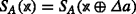
Let and . We use mathematical induction to prove that $y_{i}^{\prime }=y_{i}$ for all i. In the base step, we obtain $y_{0}^{\prime }=y_{0}$ through the equation below.

In the inductive step, we assume $y_{i}^{\prime }=y_{i}$ for all i(< t − 1) such that t < k, and we show that $y_{t}^{\prime }=y_{t}$ through the equation below.

This fact indicates that holds, regardless of . Therefore, $\delta (S_{A})=\delta _{S_{A}}({{\varDelta }} a, 0^{(k)})=2^{n}$. □

We observe how large a k is needed to eliminate all nonzero elements in the complementable space. First, let us define a matrix below.

The complementable space $\mathcal {C}_{S_{A}}$ can be defined as a homogeneous linear system as follows.

As k increases by 1, the number of rows in A increases by 2. The size of the solution space of the system A(Δa) = 0⁽ⁿ⁾ is at least 2^n− 2k. In order to become $\mathcal {C}_{S_{A}}=\{0\}$, the number of rows in A must be n or more. Since $2^{n-2\lfloor \frac {n-1}{2}\rfloor }>1$, an (n, k)-bit A-box with $k\leq \lfloor \frac {n-1}{2}\rfloor$ holds δ(S_A) = 2ⁿ by Lemma 1. Therefore, we can derive Theorem 3 as follows.

Theorem 3

Let S_A be an (n, k)-bit A-box. If $k\le \lfloor \frac {n-1}{2}\rfloor$, then δ(S_A) = 2ⁿ.

Consider an input difference Δa and an output difference Δb that comprise the differential uniformity of an A-box. When an AND gate is added, the best case is that Δa activates the last AND gate and halves the differential uniformity.

Theorem 4

Let S_A be an (n, k)-bit A-box. If $k = \lfloor \frac {n-1}{2}\rfloor +l$, then δ(S_A) ≥ 2^n−l for all l ≥ 0.

Proof

We use mathematical induction to prove this theorem from l = 0. By Theorem 3, if $k= \lfloor \frac {n-1}{2}\rfloor$, then δ(S_A) = 2ⁿ. Assume that this theorem holds when l = t. Let S_A be an (n, k + 1)-bit A-box for $k=\lfloor \frac {n-1}{2}\rfloor +t$. Then the (n, k)-bit A-box S_A|_k satisfies δ(S_A|_k) ≥ 2^n−t based on the assumption. There are two differences Δa and Δb such that $\delta _{S_{A}|_{k}}({{\varDelta }} a, {{\varDelta }} b)\ge 2^{n-t}$. We obtain the following equation.

Either $\delta _{S_{A}}({{\varDelta }} a, 0||{{\varDelta }} b)\ge 2^{n-t-1}$ or $\delta _{S_{A}}({{\varDelta }} a, 1||{{\varDelta }} b)\ge 2^{n-t-1}$ holds by the pigeonhole principle. Thus, we have δ(S_A) ≥ 2^n−t− 1. □

As previously considered, the bound of the A-box becomes the bound of the S-box. Corollary 1 follows from Theorems 1, 3, and 4.

Corollary 1

Let S be an (n, m)-bit S-box. The following properties hold.

• If $c_{\wedge }(S)\leq \lfloor \frac {n-1}{2}\rfloor$, then δ(S) = 2ⁿ.

• If $c_{\wedge }(S)=\lfloor \frac {n-1}{2}\rfloor +l$, then δ(S) ≥ 2^n−l for l ≥ 0.

3.2 Bounds for linearity

While the theoretical relationship between MC and differential uniformity has not been studied, the theoretical relationship between MC and linearity has been previously studied [10]. Boyar and Find studied the relationship using linear codes and ΣπΣ circuit. To have low linearity, more AND gates must be used than the length of the shortest corresponding linear code. For example, an (n, n)-bit S-box with linearity $2^{\frac {n-1}{2}}$ should use $L(n,\frac {n-1}{2})$ or more AND gates in the ΣπΣ circuit, where $L(n,\frac {n-1}{2})$ is the length of the shortest linear n-dimensional code over with a distance $\frac {n-1}{2}$. For a sufficiently large n, $L(n,\frac {n-1}{2})>2.32n$. However, it remains to be determined how large n must be, which makes this result difficult to apply directly to the construction of an S-box in practice. Therefore, we will more clearly present the lower bounds of linearity by MC.

For two maskings and , the linear equation of (n, m)-bit S-box S is followed.

(6)

If k < m, the last row of M is a zero row. In this case, it is easily shown that ${\mathscr{L}}_{S}({{\varLambda }} a,{{\varLambda }} b)=2^{n}$ when Λa = 0⁽ⁿ⁾ and Λb = 0^(m− 1)||1. The following theorem has been proved.

Theorem 5

Let S be an (n, m)-bit S-box. If c_∧(S) ≤ m − 1, then ${\mathscr{L}}(S)=2^{n}$.

Assume that k = m + l − 1 for l ≥ 1. Then, M is decomposed as follows.

$$ M=\begin{pmatrix} M_{0} & M_{1} \end{pmatrix} $$

where M₀ and M₁ are m × (m − 1) and m × l partition matrices, respectively. Note that the last row of M₀ is a zero row (Fig. 3).

Fig. 3

m × k matrix M decomposed by two partition matrices m × (m − 1) M₀ and m × l M₁

The (6) is expressed by

(7)

when Λb = 0^(m− 1)||1. We denote the n-variable Boolean function f as . We refer to the following theorem, which is proved in [10].

Theorem 6

Let f be an n-variable Boolean function. Then ${\mathscr{L}}(f)\ge 2^{n-c_{\wedge }(f)}$ [10].

By the definition of A-box, the MC of f is less than or equal to l. This means ${\mathscr{L}}(f)\geq 2^{n-l}$. For such that ${\mathscr{L}}(f)={\mathscr{L}}_{f}({{\varLambda }} a, 1)$, we get

$$ \begin{array}{@{}rcl@{}} \mathcal{L}(S)\geq \mathcal{L}_{S}({{\varLambda}} a, 0^{(m-1)}||1)=\mathcal{L}_{f}({{\varLambda}} a, 1)=\mathcal{L}(f)\geq2^{n-l}. \end{array} $$

We have proved Theorem 7.

Theorem 7

Let S be an (n, m)-bit S-box. If c_∧(S) = m + l − 1, then ${\mathscr{L}}(S)\ge 2^{n-l}$ for l ≥ 0.

4 Method for searching for S-boxes with low differential uniformity by MC

In [37], Zajac and Jókay presented an algorithm to construct bijective (4,4)-bit S-boxes with minimal nonlinear gates. Since their method performs an exhaustive search for S-boxes regardless of their cryptographic properties such as differential uniformity and linearity, it would be computationally difficult to apply to search for S-boxes with a size larger than 4 bits. In order to search for S-boxes with a larger size, we focus on the S-boxes with low differential uniformity. We adopt the branch-and-bound technique for our algorithm to investigate S-boxes with larger sizes.

We say that an A-box (or S-box) has a theoretically optimal differential uniformity when its differential uniformity equals the lower bound presented in Corollary 1. That is, the theoretically optimal differential uniformity of an (n, k)-bit A-box is 2^n−l for $k=\lfloor \frac {n-1}{2}\rfloor +l$.

The phases for searching the S-box with k nonlinear gates, differential uniformity δ and linearity ${\mathscr{L}}$ are as follows.

Phase 1.:

Find an (n, k)-bit A-box S_A with the desired differential uniformity δ.

• (a) Collect $(n,\lfloor \frac {n-1}{2}\rfloor +1)$-bit A-boxes with theoretically optimal differential uniformity 2^n− 1 (cf. Section 4.1).

• (b) Extend them to $(n,\lfloor \frac {n-1}{2}\rfloor +l)$-bit A-boxes with theoretically optimal differential uniformity 2^n−l, where l > 1 (cf. Algorithm 1 in Section 4.2).

• (c) Choose $(n,\lfloor \frac {n-1}{2}\rfloor +l)$-bit A-boxes with the lowest differential uniformity when Phase 1-(b) fails with respect to l. (cf. Section 4.2).

Phase 2.:

Find an m × k matrix M in RREF to make $\mathcal {T}_{M}\circ S_{A}$ with the desired differential uniformity δ and linearity ${\mathscr{L}}$ (cf. Section 4.3).

Phase 3.:

(Optional) Find an n × n matrix N to make an (n, n)-bit S-box $\mathcal {T}_{M}\circ S_{A}\oplus \mathcal {T}_{N}$ bijective, where n = m (cf. Section 4.3).

The above process is described in Fig. 4.

Fig. 4

Constructing an S-box from an A-box

4.1 $(n,\lfloor \frac {n-1}{2}\rfloor +1)$-bit A-boxes with theoretically optimal differential uniformity 2^n− 1

In order to have differential uniformity 2^n− 1, the complementable space must be {0}. That is, the rows of matrix A in Section 3.1 span the dimension n. This fact induces the following lemma.

Lemma 2

For $k=\lfloor \frac {n-1}{2}\rfloor +1$, let S_A be an (n, k)-bit A-box. If δ(S_A) = 2^n− 1, then restricted partner vectors span the dimension n.

If n vectors span dimension n, the vectors are linearly independent. These vectors can be transformed on a standard basis by operating an appropriate matrix. Note Theorem 2. If we compose $\mathcal {T}_{L}$ on the input of the S_A, we can get a linear equivalent A-box that has the matrix-operated partner vectors. Specifically, the restricted partner vector is transformed into for all i ≥ 0. In Lemma 2, if n is even, the restricted partner vectors span the dimension n. All of the n vectors can be transformed on a standard basis through an appropriate $\mathcal {T}_{L}$. However, if n is odd, the n + 1 vectors span the dimension n, so they are linearly dependent. In this case, it can be resolved by removing the vector that causes the linear dependence. Owing to this difference, the partner vectors have a different form depending on whether n is even or odd.

Theorem 8

Let n = 2p for p > 0. For k = p, let S_A be an (n, k)-bit A-box such that δ(S_A) = 2^n− 1. Then, there is an A-box $S_{A}^{\prime }$, which is linear equivalent to S_A and has a partner tuple such that

where e_i is the n-bit value whose bits are all zeros except for the i^th-bit (e.g., e₀ = (0, ⋯ , 0, 1)).

Proof

Let us define an n × n matrix B as follows using the partner vectors of S_A.

According to Lemma 2, spans the dimension n and B is invertible. holds for all i(< n), because it is the i^th column of the identity matrix. By Theorem 2, the A-box $S_{A}^{\prime }=S_{A}\circ \mathcal {T}_{B^{-T}}$ is an A-box linear equivalent to S_A.

By the same theorem, we know that and . Note that the A-box S_A is invariant when and are swapped. We Assume, without loss of generality, for 0 < i < p in integer form. $S_{A}^{\prime }$ satisfies all required conditions. □

Theorem 9

Let n = 2p + 1 for p > 0. For k = p + 1, let S_A be an (n, k)-bit A-box such that δ(S_A) = 2^n− 1. Then, there is an A-box $S_{A}^{\prime }$, which is linear equivalent to S_A and has a partner tuple such that

where is a j-bit string and j is the largest subscript that causes linear dependence for a set of n + 1 vectors: .

Proof

As the n + 1 vectors are linearly dependent, there exist some such that

(8)

Let c_j be the nonzero coefficient with the highest subscript j. We obtain the following:

If j is 0, then and y₀ = 0. As this induces c_∧(S_A) ≤ p − 1, we obtain δ(S_A) ≥ 2^n+ 1 by Corollary 1. However, this contradicts the assumption. If j = 1, then . When c₀ = 0, we have the same case as when j = 0. c₀ = 1 makes y₀ a linear function, as shown below.

This induces c_∧(S_A) ≤ p + l − 1 and causes a contradiction, too. Therefore, we have found that j ≥ 2.

are linearly independent because they span the dimension n by Lemma 2. Let us make the following invertible matrix C

where ρ_j(i) = { i for i < j i + 1 for i ≥ j. We know that for i(< n). By Theorem 2, $S_{A}^{\prime }=S_{A}\circ \mathcal {T}_{C^{-T}}$ is an A-box that is linear equivalent to S_A. $S_{A}^{\prime }$ also satisfies the first required condition.

Next, let us see what form becomes. Let for . Then, the property below follows.

As the above property must hold for every , we obtain

Since j must be the highest subscript in the equation, we get

$$ d_{n-1}=d_{n-2}=\cdots=d_{j}=0. $$

Therefore,

As in the previous proof, assuming for i≠j, j + 1 and 0 < i ≤ p, $S_{A}^{\prime }$ satisfies all required conditions. □

These theorems enable us to significantly reduce the search space for possible $(n,\lfloor \frac {n-1}{2}\rfloor +1)$-bit A-boxes with differential uniformity 2^n− 1 (Fig. 5). Table 3 presents the A-box search space, which excludes duplication, and the number of A-boxes with theoretically optimal differential uniformity.

Fig. 5

A-boxes defined by Theorems 8 and 9

Table 3 $(n,\lfloor \frac {n-1}{2}\rfloor +1)$-bit A-box search

4.2 Extending A-boxes with theoretically optimal differential uniformity by MC

We extend A-boxes by increasing AND gates step by step. Adding one AND gate to an (n, k)-bit A-box is the same as determining two additional partner vectors and . In order to obtain an extended A-box with theoretically optimal differential uniformity, the A-box in a previous step must have theoretically optimal differential uniformity. This condition follows from the below theorem.

Theorem 10

For $k=\lfloor \frac {n-1}{2}\rfloor +l$, let S_A be an (n, k)-bit A-box for l ≥ 0. If δ(S_A) = 2^n−l, then δ(S_A|_k−p) = 2^n−l+p for all p ≤ l.

Proof

Note that the A-box S_A|_k−p is constructed by removing the last p-bits (p MSBs) generated from the S_A. As S_A|_k−p is an (n, k − p)-bit A-box, δ(S_A|_k−p) ≥ 2^n−l+p holds by Theorem 4. Assume that $\delta (S_{A}|_{k-p})\gneq 2^{n-l+p}$. There are two differences Δa and Δb such that $\delta (S_{A}|_{k-p})=\delta _{S_{A}|_{k-p}}({{\varDelta }} a,{{\varDelta }} b)$. According to the definition of an A-box, the following equation holds.

Next, we obtain

As $\delta _{S_{A}|_{k-p}}({{\varDelta }} a,{{\varDelta }} b)>2^{n-l+p}$, there is a vector that satisfies

by the pigeonhole principle. As a result, we have , but this contradicts the assumption. □

Therefore, we can accelerate the investigation by checking whether the differential uniformity of the A-boxes constructed in each step is theoretically optimal.

In Section 4.1, we obtained a set of $(n,\lfloor \frac {n-1}{2}\rfloor +1)$-bit A-boxes with theoretically optimal differential uniformity 2^n− 1. We call this set $\mathcal {A}$ and refer to A-boxes of $\mathcal {A}$ as parent nodes. A child node is an A-box with one AND gate added to a parent node. The number of child nodes per parent node is as many as two additional partner vectors and are possible for adding k^th AND gate (cf. Fig. 6). To count the number of A-boxes per depth, our algorithm performs a breadth-first search. The detailed process is described in Algorithm 1.

Fig. 6

A-box extension ((n, k + 1)-bit $S_{A}^{\prime }$ extended from (n, k)-bit S_A)

In the algorithm, the partner vectors and are handled in integer form. There are two reasons why starts at :

• Since , generality is not lost even if .

• Since , the case does not need to be investigated.

The number of A-boxes with theoretically optimal differential uniformity at each step is listed in Table 4. For 5-, 6-, and 8-bit sizes, our algorithm shows the following facts. The symbol ‘∗’ means that any number is possible.

• A (5,∗)-bit S-box with differential uniformity 2 has MC at least 7.

• A (6,∗)-bit S-box with differential uniformity 4 has MC at least 7.

• An (8,∗)-bit S-box with differential uniformity 32 has MC at least 7.

Table 4 Number of partner tuples that construct A-boxes with theoretically optimal differential uniformity

This result also shows that Phase 1-(b) can fail. In this case, we chose the A-boxes with the lowest differential uniformity to construct the corresponding S-boxes.

4.3 Construction of S-boxes by A-boxes

Generating the m × k matrix M in RREF is simple. If k ≤ m, M consists only of pivot columns. The differential uniformity of $\mathcal {T}_{M}\circ S_{A}$ equals the differential uniformity of S_A. The linearity is at most 2ⁿ − 1 as per Theorem 7. Let k > m. The columns of M are divided into m pivot columns and k − m other columns. We randomly select the pivot columns and then randomly generate other columns. After arranging the pivot columns in order of subscript, the other columns are inserted randomly to generate a matrix. When M is generated, we calculate whether the differential uniformity and linearity of $\mathcal {T}_{M}\circ S_{A}$ are the desired values.

A bijective S-box is more useful than a non-bijective one when it has the same cryptographic properties. In particular, for the efficiency of side-channel masking, it is recommended to use an S-box with low MC as the primitive. For example, the block cipher Pyjamask [24], proposed in the recent NIST lightweight encryption competition, uses small S-boxes of (3,3)-bit and (4,4)-bit sizes to improve the side-channel masking efficiency. Fantomas and Robin [25] proposed LS-designs, which use bijective (8,8)-bit S-boxes generated from an extension structure to reduce the number of nonlinear gates.

Let S be an (n, n)-bit S-box. Note that where N is an n × n matrix. We denote the entry of row i and column j of N by N_{i, j}. As $\mathcal {T}_{D}$ is bijective, the expression of S can be transformed as follows.

In the equation above, the bijectivity of S is expressed by $\mathcal {T}_{M}\circ S_{A}\oplus \mathcal {T}_{D}^{-1}\circ \mathcal {T}_{N}$. Finding $\mathcal {T}_{D}^{-1}\circ \mathcal {T}_{N}$ is the same as finding the n × n matrix, so we can regard it as $\mathcal {T}_{N}$. Therefore, our goal is to find the $\mathcal {T}_{N}$ that makes $\mathcal {T}_{M}\circ S_{A}\oplus \mathcal {T}_{N}$ bijective.

A bijective S-box has the characteristic that any combination of output bits is balanced. The new (n, d)-bit S-box (f_σ(d− 1), ⋯ , f_σ(0)), generated by choosing d random f_i for the bijective (n, n)-bit S-box S = (f_n− 1, ⋯ , f₀), is balanced (σ is a permutation of ). Let and . Then, for i(< n), z_i is as follows:

$$ \begin{array}{@{}rcl@{}} z_{i}=y_{i}\oplus \bigoplus_{j=0}^{n-1} N_{j,i}x_{j} \end{array} $$

We first investigate (N_{n− 1, n− 1}, ⋯ , N_n− 1,1, N_{n− 1, 0}) where is balanced. Second, we investigate (N_{n− 1, n− 1}, ⋯ , N_n− 1,1, N_{n− 1, 0}) and (N_{n− 2, n− 1}, ⋯ , N_n− 2,1, N_{n− 2, 0}) where is balanced. By repeating this process, we can find the N where becomes bijective.

5 Conclusions

In this paper, we proved the theoretical lower bounds of differential uniformity and linearity of S-boxes by MC. We also presented an algorithm to search A-boxes with theoretically optimal differential uniformity by MC. The constructed A-boxes lead to S-boxes through our process. Some of the bijective S-boxes we found have better differential uniformity than those of existing bijective S-boxes with respect to the same nonlinear gates and linearity. Using our process, cryptography designers can make a trade-off between the implementation efficiency and security of the S-box, and they can reduce the complexity of S-box investigation because the minimum MC of the S-box having the desired security is known in advance based on this paper.

In future work, it would be interesting to investigate the following research topics:

• From a hardware point of view, is there a way to construct A-box to have high security but low AND depth?

• Is there a better way than a random process to construct S-boxes from a fixed A-box?

• How does bijectivity theoretically relate to A-boxes?

• How do the nonlinear gates of an A-box relate to other cryptographic properties such as algebraic degree, fixed points, or other properties?

Appendix A: Bitsliced implementations of our S-boxes

In this appendix, the method to implement the S-boxes presented in Table 2, which we found by experiments, is shown in Listing 1∼7.

Listing 1

5-bit S-box with MC 4 (Differential uniformity 8, Linearity 32

These are written in the C language. In each listing, X is an input bit string, Y is an output bit string, and T is a temporary bit string.

Listing 2

6-bit S-box with MC 6 (Differential uniformity 8, Linearity 32)

Listing 3

6-bit S-box with MC 7 (Differential uniformity 4, Linearity 16)

Listing 4

7-bit S-box with MC 5 (Differential uniformity 32, Linearity 128)

Listing 5

7-bit S-box with MC 10 (Differential uniformity 4, Linearity 32)

Listing 6

8-bit S-box with MC 8 (Differential uniformity 16, Linearity 128)

Listing 7

8-bit S-box with MC 10 (Differential uniformity 8, Linearity 128)

References

Adomnicai, A., Berger, T.P., Clavier, C., Francq, J., Huynh, P., Lallemand, V., Le Gouguec, K., Minier, M., Reynaud, L., Thomas, G.: Lilliput-AE: a new lightweight tweakable block cipher for authenticated encryption with associated data. Submitted to NIST Lightweight Project (2019)
Albrecht, M.R., Rechberger, C., Schneider, T., Tiessen, T., Zohner, M.: Ciphers for MPC and FHE. In: Oswald, E., Fischlin, M. (eds.) Advances in Cryptology - EUROCRYPT 2015 - 34th Annual International Conference on the Theory and Applications of Cryptographic Techniques, Sofia, Bulgaria, April 26-30, 2015, Proceedings, Part I, Lecture Notes in Computer Science, vol. 9056, pp. 430–454. Springer. https://doi.org/10.1007/978-3-662-46800-5_17 (2015)
Andreeva, E., Bilgin, B., Bogdanov, A., Luykx, A., Mendel, F., Mennink, B., Mouha, N., Wang, Q., Yasuda, K.: PRIMATEs v1.02. CAESAR submission. http://competitions.cr.yp.to/round2/primatesv102.pdf (2015)
Beierle, C., Jean, J., Kölbl, S., Leander, G., Moradi, A., Peyrin, T., Sasaki, Y., Sasdrich, P., Sim, S.M.: The SKINNY family of block ciphers and its low-latency variant MANTIS. In: Robshaw, M., Katz, J. (eds.) Advances in Cryptology - CRYPTO 2016 - 36th Annual International Cryptology Conference, Santa Barbara, CA, USA, August 14-18, 2016, Proceedings, Part II, Lecture Notes in Computer Science, vol. 9815, pp. 123–153. Springer. https://doi.org/10.1007/978-3-662-53008-5_5(2016)
Berger, T.P., Canteaut, A., Charpin, P., Laigle-Chapuy, Y.: On almost perfect nonlinear functions over \(\text {F}_{2}^{\text {n}}\). IEEE Trans. Inf. Theory 52 (9), 4160–4170 (2006). https://doi.org/10.1109/TIT.2006.880036
Biham, E., Shamir, A.: Differential cryptanalysis of DES-like cryptosystems. In: Menezes, A., Vanstone, S.A. (eds.) Advances in Cryptology - CRYPTO ’90, 10th Annual International Cryptology Conference, Santa Barbara, California, USA, August 11-15, 1990, Proceedings, Lecture Notes in Computer Science, vol. 537, pp. 2–21. Springer. https://doi.org/10.1007/3-540-38424-3_1 (1990)
Bilgin, B., Meyer, L.D., Duval, S., Levi, I., Standaert, F.: Low AND depth and efficient inverses: a guide on S-boxes for low-latency masking. IACR Trans. Symmetric Cryptol. 2020(1), 144–184 (2020). https://doi.org/10.13154/tosc.v2020.i1.144-184
Bilgin, B., Nikova, S., Nikov, V., Rijmen, V., Stütz, G.: Threshold implementations of all 3 ×3 and 4 ×4 S-boxes. In: Prouff, E., Schaumont, P. (eds.) Cryptographic Hardware and Embedded Systems - CHES 2012 - 14th International Workshop, Leuven, Belgium, September 9-12, 2012. Proceedings, Lecture Notes in Computer Science, vol. 7428, pp. 76–91. Springer. https://doi.org/10.1007/978-3-642-33027-8_5 (2012)
Bogdanov, A., Knudsen, L.R., Leander, G., Paar, C., Poschmann, A., Robshaw, M.J.B., Seurin, Y., Vikkelsoe, C.: PRESENT: An ultra-lightweight block cipher. In: Paillier, P., Verbauwhede, I. (eds.) Cryptographic Hardware and Embedded Systems - CHES 2007, 9th International Workshop, Vienna, Austria, September 10-13, 2007, Proceedings, Lecture Notes in Computer Science, vol. 4727, pp. 450–466. Springer. https://doi.org/10.1007/978-3-540-74735-2_31 (2007)
Boyar, J., Find, M.G.: Multiplicative complexity of vector valued Boolean functions. Theor. Comput. Sci. 720, 36–46 (2018). https://doi.org/10.1016/j.tcs.2018.02.023
Boyar, J., Matthews, P., Peralta, R.: Logic minimization techniques with applications to cryptology. J. Cryptol. 26(2), 280–312 (2013). https://doi.org/10.1007/s00145-012-9124-7
Boyar, J., Peralta, R.: Concrete multiplicative complexity of symmetric functions. In: Kralovic, R., Urzyczyn, P. (eds.) Mathematical Foundations of Computer Science 2006, 31st International Symposium, MFCS 2006, Stará Lesná, Slovakia, August 28-September 1, 2006, Proceedings, Lecture Notes in Computer Science, vol. 4162, pp. 179–189. Springer. https://doi.org/10.1007/11821069_16 (2006)
Boyar, J., Peralta, R., Pochuev, D.: On the multiplicative complexity of Boolean functions over the basis (∧, ⊕, 1). Theor. Comput. Sci. 235(1), 43–57 (2000). https://doi.org/10.1016/S0304-3975(99)00182-6
Bozilov, D., Bilgin, B., Sahin, H.A.: A note on 5-bit quadratic permutations’ classification. IACR Trans. Symmetric Cryptol. 2017(1), 398–404 (2017). https://doi.org/10.13154/tosc.v2017.i1.398-404
Canteaut, A., Perrin, L.: On CCZ-equivalence, extended-affine equivalence, and function twisting. Finite Fields Their Appl. 56, 209–246 (2019). https://doi.org/10.1016/j.ffa.2018.11.008
Carlet, C., Ding, C.: Nonlinearities of S-boxes. Finite Fields Their Appl. 13(1), 121–135 (2007). https://doi.org/10.1016/j.ffa.2005.07.003
Chabaud, F., Vaudenay, S.: Links between differential and linear cryptanalysis. In: Santis, A.D. (ed.) Advances in Cryptology - EUROCRYPT ’94, Workshop on the Theory and Application of Cryptographic Techniques, Perugia, Italy, May 9-12, 1994, Proceedings, Lecture Notes in Computer Science, vol. 950, pp. 356–365. Springer. https://doi.org/10.1007/BFb0053450 (1994)
Chase, M., Derler, D., Goldfeder, S., Orlandi, C., Ramacher, S., Rechberger, C., Slamanig, D., Zaverucha, G.: Post-quantum zero-knowledge and signatures from symmetric-key primitives. In: Thuraisingham, B.M., Evans, D., Malkin, T., Xu, D. (eds.) Proceedings of the 2017 ACM SIGSAC Conference on Computer and Communications Security, CCS 2017, Dallas, TX, USA, October 30 - November 03, 2017, pp. 1825–1842. ACM. https://doi.org/10.1145/3133956.3133997 (2017)
Courtois, N., Mourouzis, T., Hulme, D.: Exact logic minimization and multiplicative complexity of concrete algebraic and cryptographic circuits. Int. J. Adv. Intell. Syst. 6(3), 165–176 (2013)
Courtois, N.T.: How fast can be algebraic attacks on block ciphers? In: Biham, E., Handschuh, H., Lucks, S., Rijmen, V. (eds.) Symmetric Cryptography, 07.01. - 12.01.2007, Dagstuhl Seminar Proceedings, vol. 07021. Internationales Begegnungs- und Forschungszentrum fuer Informatik (IBFI), Schloss Dagstuhl, Germany. http://drops.dagstuhl.de/opus/volltexte/2007/1013 (2007)
Courtois, N.T., Hulme, D., Mourouzis, T.: Solving Circuit Optimisation Problems in Cryptography and Cryptanalysis. IACR Cryptol. ePrint Arch. 2011, 475. http://eprint.iacr.org/2011/475 (2011)
Daemen, J., Rijmen, V.: The block cipher rijndael. In: Quisquater, J., Schneier, B. (eds.) Smart Card Research and Applications, This International Conference, CARDIS ’98, Louvain-la-Neuve, Belgium, September 14-16, 1998, Proceedings, Lecture Notes in Computer Science, vol. 1820, pp. 277–284. Springer. https://doi.org/10.1007/10721064_26 (1998)
Giacomelli, I., Madsen, J., Orlandi, C.: ZKBoo: Faster zero-knowledge for boolean circuits. In: Holz, T., Savage, S. (eds.) 25th USENIX Security Symposium, USENIX Security 16, Austin, TX, USA, August 10-12, 2016, pp. 1069–1083. USENIX Association. https://www.usenix.org/conference/usenixsecurity16/technical-sessions/presentation/giacomelli (2016)
Goudarzi, D., Jean, J., Kölbl, S., Peyrin, T., Rivain, M., Sasaki, Y., Sim, S.M.: Pyjamask: Block Cipher and Authenticated Encryption with Highly Efficient Masked Implementation. IACR Trans. Symmetric Cryptol. 2020 (S1), 31–59 (2020). https://doi.org/10.13154/tosc.v2020.iS1.31-59
Grosso, V., Leurent, G., Standaert, F., Varici, K.: LS-designs: Bitslice encryption for efficient masked software implementations. In: Cid, C., Rechberger, C. (eds.) Fast Software Encryption - 21st International Workshop, FSE 2014, London, UK, March 3-5, 2014. Revised Selected Papers, Lecture Notes in Computer Science, vol. 8540, pp. 18–37. Springer. https://doi.org/10.1007/978-3-662-46706-0_2 (2014)
Halevi, S., Shoup, V.: Algorithms in HElib. In: Garay, J.A., Gennaro, R. (eds.) Advances in Cryptology - CRYPTO 2014 - 34th Annual Cryptology Conference, Santa Barbara, CA, USA, August 17-21, 2014, Proceedings, Part I, Lecture Notes in Computer Science, vol. 8616, pp. 554–571. Springer. https://doi.org/10.1007/978-3-662-44371-2_31 (2014)
Hatzivasilis, G., Fysarakis, K., Papaefstathiou, I., Manifavas, C.: A review of lightweight block ciphers. J. Cryptogr. Eng. 8(2), 141–184 (2018). https://doi.org/10.1007/s13389-017-0160-y
Kim, H., Jeon, Y., Kim, G., Kim, J., Sim, B., Han, D., Seo, H., Kim, S., Hong, S., Sung, J., Hong, D.: A New Method for Designing Lightweight S-boxes with High Differential and Linear Branch Numbers, and Its Application. IACR Cryptol. ePrint Arch. 2020, 1582. https://eprint.iacr.org/2020/1582 (2020)
Kocher, P.C.: Timing attacks on implementations of Diffie-Hellman, RSA, DSS, and other systems. In: Koblitz, N. (ed.) Advances in Cryptology - CRYPTO ’96, 16th Annual International Cryptology Conference, Santa Barbara, California, USA, August 18-22, 1996, Proceedings, Lecture Notes in Computer Science, vol. 1109, pp. 104–113. Springer. https://doi.org/10.1007/3-540-68697-5_9 (1996)
Kolesnikov, V., Schneider, T.: Improved garbled circuit: Free XOR gates and applications. In: Aceto, L., Damgård, I., Goldberg, L.A., Halldórsson, M.M., Ingólfsdóttir, A., Walukiewicz, I. (eds.) Automata, Languages and Programming, 35th International Colloquium, ICALP 2008, Reykjavik, Iceland, July 7-11, 2008, Proceedings, Part II - Track B: Logic, Semantics, and Theory of Programming & Track C: Security and Cryptography Foundations, Lecture Notes in Computer Science, vol. 5126, pp. 486–498. Springer. https://doi.org/10.1007/978-3-540-70583-3_40 (2008)
Matsui, M.: Linear Cryptanalysis Method for DES Cipher. In: Helleseth, T. (ed.) Advances in Cryptology - EUROCRYPT ’93, Workshop on the Theory and Application of of Cryptographic Techniques, Lofthus, Norway, May 23-27, 1993, Proceedings, Lecture Notes in Computer Science, vol. 765, pp. 386–397. Springer. https://doi.org/10.1007/3-540-48285-7_33 (1993)
Songhori, E.M., Hussain, S.U., Sadeghi, A., Schneider, T., Koushanfar, F.: TinyGarble: Highly Compressed and Scalable Sequential Garbled Circuits. In: 2015 IEEE Symposium on Security and Privacy, SP 2015, San Jose, CA, USA, May 17-21, 2015, pp. 411–428. IEEE Computer Society. https://doi.org/10.1109/SP.2015.32 (2015)
Stoffelen, K.: Optimizing s-box implementations for several criteria using SAT solvers. In: Peyrin, T. (ed.) Fast Software Encryption - 23rd International Conference, FSE 2016, Bochum, Germany, March 20-23, 2016, Revised Selected Papers, Lecture Notes in Computer Science, vol. 9783, pp. 140–160. Springer. https://doi.org/10.1007/978-3-662-52993-5_8 (2016)
Testa, E., Soeken, M., Amarù, L. G., Micheli, G.D.: Reducing the Multiplicative Complexity in Logic Networks for Cryptography and Security Applications. In: Proceedings of the 56th Annual Design Automation Conference 2019, DAC 2019, Las Vegas, NV, USA, June 02-06, 2019, p. 74. ACM. https://doi.org/10.1145/3316781.3317893 (2019)
Yao, A.C.: How to generate and exchange secrets (extended abstract). In: 27th Annual Symposium on Foundations of Computer Science, Toronto, Canada, 27-29 October 1986, pp. 162–167. IEEE Computer Society. https://doi.org/10.1109/SFCS.1986.25(1986)
Zajac, P.: Constructing S-boxes with low multiplicative complexity. Stud. Sci. Math. Hung. 52(2), 135–153 (2015)
Zajac, P., Jókay, M.: Multiplicative complexity of bijective 4×4 S-boxes. Cryptogr. Commun. 6 (3), 255–277 (2014). https://doi.org/10.1007/s12095-014-0100-y
Acknowledgements
This work was supported by Institute for Information & communications Technology Promotion(IITP) grant funded by the Korea government(MSIT) (No.2017-0-00520, Development of SCR-Friendly Symmetric Key Cryptosystem and Its Application Modes)
Author information
Authors and Affiliations
Corresponding author
Additional information
Publisher’s note
Springer Nature remains neutral with regard to jurisdictional claims in published maps and institutional affiliations.