Natural Deduction for Quantum Logic

Abstract

This paper presents a natural deduction system for orthomodular quantum logic. The system is shown to be provably equivalent to Nishimura’s quantum sequent calculus. Through the Curry–Howard isomorphism, quantum $\lambda$-calculus is also introduced for which strong normalization property is established.

1 Introduction

This paper presents a natural deduction system for orthomodular quantum logic. The main contributions of the system are as follows. First, thanks to its intrinsic and straightforward appearance, we can understand the meaning of inference in quantum logic deeply by comparing the system with those for other logics (e.g. intuitionistic logic or classical logic). Second, we can also introduce the corresponding quantum $\lambda$-calculus, which allows us to further investigate computational theories based on quantum logic, via the Curry–Howard isomorphism. Third, we can establish a desirable property regarding normalization of proofs, or equivalently, termination of computation.

As an earlier study for quantum natural deduction, we need to mention Delmas-Rigoutsos’s double deduction system [5], which incorporates a concept of compatibility into a natural deduction system for classical logic. Differently from this approach, we define a natural deduction system that directly corresponds to GOM, Nishimura’s quantum sequent calculus [13].

Besides GOM, a few systems for quantum sequent calculus have been proposed by Cutland and Gibbins [3] and Nishimura [14]. Furthermore, an extended logical system containing quantum logic called basic logic along with its sequent calculus has been studied by Sambin et al. [19], Faggian and Sambin [7], and Dalla Chiara and Giuntini [4]. These systems, however, are all inadequate for being translated into natural deduction forms due to their complex treatment of negation ($\lnot$) and cut.

It is known that quantum logic has no satisfactory implication operation ($\rightarrow$) as in the case of intuitionistic logic or classical logic. Indeed, Nishimura’s GOM only adopts conjunction ($\wedge$) and negation ($\lnot$) as the basic set of operations. On the other hand, it is almost inevitable to include implication in the basic set of operations for the purpose of developing a natural deduction system and the corresponding $\lambda$-calculus. To handle such a contradiction, we employ the Sasaki hook, a kind of quasi-implication, as one of the basic operations of our system. Although it fails to satisfy the deduction theorem, the Sasaki hook still enjoys some expected properties of implication such as modus ponens. The problem of implication in quantum logic is what has been largely addressed in the literature; for details, the reader is referred to Hardegree [9], Herman et al. [11], Pavičić [15], Malinowski [12], Pavičić and Megill [16], Roman and Zuazua [18], Ying [22], Chajda and Halaš [1], Harding [10], Chajda [2], and Younes and Schmitt [23].

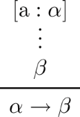
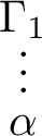
Another problem that we encounter when associating GOM with a natural deduction system is how to treat assumptions in a deduction process. In the usual natural deduction system for intuitionistic logic or classical logic, assumptions that are not used in the application of a rule may be omitted. That is, for example:

(1)

In this case, it is legitimate that assumptions other than $\alpha$ are not explicitly stated even if they exist. The point becomes clear when we express this situation in the sequent calculus form:

Here, all (undischarged) assumptions other than $\alpha$ are explicitly written as $\Gamma$, a (possibly empty) set of formulas.

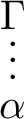
In quantum logic, however, the introduction rule of implication (the Sasaki hook) is subject to a restriction due to the failure of the deduction theorem. That is, the introduction rule of implication (1) can only be applied if there exist no assumptions other than $\alpha$. Again, we view this as a sequent calculus form:

Taking this restriction into account, we will use the following convention in defining and applying rules of our natural deduction system: the assumptions that are not explicitly stated must not exist. When written in this style, the introduction rule of implication (1) in intuitionistic logic or classical logic would become as follows:

(2)

Let us give an example of a proof diagram. The following proof is legitimate in intuitionistic or classical logic:

Here, $\mathrm {a}$, $\mathrm {b}$, and $\mathrm {c}$ are labels, which are used to identify assumptions to be discharged.

However, the proof above is illegitimate in quantum logic, as the rule labeled by ($\mathrm {a}$) must not be applied due to the existence of assumptions $\mathrm {b}$ and $\mathrm {c}$ remaining undischarged at this point:

Indeed, the proposition $(\alpha \rightarrow \beta ) \rightarrow ((\beta \rightarrow \gamma ) \rightarrow (\alpha \rightarrow \gamma ))$ is not a theorem of quantum logic. It can therefore be said that quantum logic is non-monotonic in the sense that adding assumptions might interfere with a deduction process.

A difference in the treatment of assumptions between natural deduction and sequent calculus has been mentioned in Restall [17]. Monotonicity in quantum logic has been pointed out in the context of quantum uncertainty in Engesser et al. [6].

Once a natural deduction system for quantum logic is obtained, the corresponding quantum $\lambda$-calculus can be introduced via the Curry–Howard isomorphism: the proofs of the natural deduction system can be reversibly translated into the terms of the $\lambda$-calculus, respectively. Finally, we will prove the strong normalization property for the quantum $\lambda$-calculus, which claims that any computation in the quantum $\lambda$-calculus eventually terminates.

The quantum $\lambda$-calculus introduced in this paper is based on orthomodular quantum logic, while several other systems based on intuitionistic linear logic have also been studied under the name quantum $\lambda$-calculus [20, 21]. The proof of the strong normalization property presented in this paper follows that of Girard et al. [8].

The organization of this paper is as follows: Sect. 2 provides a formal definition of NQ, a natural deduction system for quantum logic. Section 3 shows the equivalence between NQ and GOM. Section 4 introduces the corresponding quantum $\lambda$-calculus together with the Curry–Howard isomorphism from NQ. Section 5 establishes a rigorous proof of the strong normalization property for the quantum $\lambda$-calculus. The last section draws a conclusion.

2 Formal Definition of NQ

This section provides a formal definition of NQ, a natural deduction system for quantum logic. To begin with, we construct formulas over a countable set of propositional variables and a propositional constant $\bot$.

Definition 2.1

(Formula). Formulas are inductively defined as follows:

• $\alpha$ is a formula if $\alpha$ is a propositional variable.

• $\alpha$ is a formula if $\alpha$ is $\bot$.

• $(\alpha \wedge \beta )$ is a formula if $\alpha$ and $\beta$ are formulas.

• $(\alpha \rightarrow \beta )$ is a formula if $\alpha$ and $\beta$ are formulas.

• Only strings obtained by finitely many applications of the above rules are formulas.

Parentheses are omitted if there is no ambiguity.

We employ $\wedge$ (conjunction) and $\rightarrow$ (implication) as the basic connectives, and introduce the following as abbreviations:

• $\alpha \vee \beta \equiv \lnot (\lnot \alpha \wedge \lnot \beta )$ (disjunction)

• $\lnot \alpha \equiv \alpha \rightarrow \bot$ (negation)

The lower-case Greek letters $\alpha , \beta , \gamma , \delta$ and those with subscripts like $\alpha _1, \alpha _2, \dots$ are used to denote metavariables representing formulas; the upper-case Greek letters $\Gamma , \Delta , \Pi , \Sigma$ and those with subscripts like $\Gamma _1, \Gamma _2, \dots$ are used to denote metavariables representing finite (possibly empty) sets of formulas. $\{ \alpha \}$ and $\{ \alpha \} \cup \Gamma$ are usually abbreviated to $\alpha$ and $\alpha , \Gamma$, respectively. $\lnot \Gamma$ is a shorthand notation for $\{ \lnot \alpha \mid \alpha \in \Gamma \}$.

Definition 2.2

(Subformula). Let $\alpha$ be a formula. $\beta$ is said to be a subformula of $\alpha$ if $\beta$ is a substring of $\alpha$ and $\beta$ itself is a formula.

Definition 2.3

(Label). Labels are used to indicate assumptions in a proof. $\mathrm{a}:\alpha$ denotes an assumption where $\mathrm{a}$ is a label and $\alpha$ is a formula.

We fix a countable set of labels, so that different formulas correspond to different labels.

Definition 2.4

(Proof of NQ). In NQ, a conclusion $\alpha$ is said to be provable from a set $\Gamma$ of assumptions if there exists a proof diagram that derives $\alpha$ from $\Gamma$. Proof diagrams (or simply proofs) of NQ are inductively defined by the following rules.

• Assumption rule

  $$\begin{aligned} \mathrm{a}:\alpha \end{aligned}$$

  or

  $$\begin{aligned} \alpha \end{aligned}$$

  when the label is omitted, is a (trivial) proof that derives $\alpha$ from $\alpha$. This proof is referred to as $\mathbf {ASM}($a$:\alpha /\alpha )$.

• $\bot$-rule If

  

  is a proof, say P, that derives $\bot$ from $\Gamma$, then

  

  is a proof that derives $\alpha$ from $\Gamma$. This proof is referred to as $\mathbf{EFQ}(P/\alpha )$.

• $\mathrm{\wedge El}$-rule If

  

  is a proof that derives $\gamma$ from $\{\mathrm{a}:\alpha \} \cup \Gamma _1$, and if

  

  is a proof that derives $\alpha \wedge \beta$ from $\Gamma _2$, then

  

  is a proof that derives $\gamma$ from $\Gamma _1 \cup \Gamma _2$. Here, $[\mathrm{a}:\alpha ]$ represents a discharged assumption. This rule can be replaced by the following simpler one. If

  

  is a proof, say P, that derives $\alpha \wedge \beta$ from $\Gamma$, then

  

  is a proof that derives $\alpha$ from $\Gamma$. This proof is referred to as $\mathbf{\wedge El}(P/\alpha )$.

• $\mathrm{\wedge Er}$-rule If

  

  is a proof that derives $\gamma$ from $\{\mathrm{a}:\beta \} \cup \Gamma _1$, and if

  

  is a proof that derives $\alpha \wedge \beta$ from $\Gamma _2$, then

  

  is a proof that derives $\gamma$ from $\Gamma _1 \cup \Gamma _2$. This rule can be replaced by the following simpler one. If

  

  is a proof, say P, that derives $\alpha \wedge \beta$ from $\Gamma$, then

  

  is a proof that derives $\beta$ from $\Gamma$. This proof is referred to as $\mathbf{\wedge Er}(P/\beta )$.

• $\mathrm{\wedge I}$-rule If

  

  is a proof, say $P_1$, that derives $\alpha$ from $\Gamma _1$, and if

  

  is a proof, say $P_2$, that derives $\beta$ from $\Gamma _2$, then

  

  is a proof that derives $\alpha \wedge \beta$ from $\Gamma _1 \cup \Gamma _2$. This proof is referred to as $\mathbf{\wedge I}(P_1, P_2/\alpha \wedge \beta )$.

• $\mathrm{\rightarrow E}$-rule (Modus Ponens) If

  

  is a proof, say $P_1$, that derives $\alpha \rightarrow \beta$ from $\Gamma _1$, and if

  

  is a proof, say $P_2$, that derives $\alpha$ from $\Gamma _2$, then

  

  is a proof that derives $\beta$ from $\Gamma _1 \cup \Gamma _2$. This proof is referred to as $\mathbf{\rightarrow E}(P_1, P_2/\beta )$.

• $\mathrm{\rightarrow I}$-rule If

  

  is a proof, say P, that derives $\beta$ from $\alpha$, then

  

  is a proof that derives $\alpha \rightarrow \beta$ from no assumptions. This proof is referred to as $\mathbf{\rightarrow I}(P[\mathrm{a}:\alpha ]/\alpha \rightarrow \beta )$. As noted in Sect. 1, no assumptions other than $\mathrm{a}:\alpha$ are allowed to be made when this rule is applied.

• MT (Modus Tollens) If

  

  is a proof, say $P_1$, that derives $\alpha \rightarrow \beta$ from no assumptions, and if

  

  is a proof, say $P_2$, that derives $\beta \rightarrow \bot$ from $\Gamma$, then

  

  is a proof that derives $\alpha \rightarrow \bot$ from $\Gamma$. This proof is referred to as $\mathbf{MT}(P_1, P_2/\alpha \rightarrow \bot )$.

• $\mathrm{\lnot \lnot E}$-rule If

  

  is a proof that derives $\gamma$ from $\{\mathrm{a}:\alpha \} \cup \Gamma _1$, and if

  

  is a proof that derives $(\alpha \rightarrow \bot ) \rightarrow \bot$ from $\Gamma _2$, then

  

  is a proof that derives $\gamma$ from $\Gamma _1 \cup \Gamma _2$. This rule can be replaced by the following simpler one. If

  

  is a proof, say P, that derives $(\alpha \rightarrow \bot ) \rightarrow \bot$ from $\Gamma$, then

  

  is a proof that derives $\alpha$ from $\Gamma$. This proof is referred to as $\mathbf{\lnot \lnot E}(P/\alpha )$.

• $\mathrm{\lnot \lnot I}$-rule If

  

  is a proof, say P, that derives $\alpha$ from $\Gamma$, then

  

  is a proof that derives $(\alpha \rightarrow \bot ) \rightarrow \bot$ from $\Gamma$. This proof is referred to as $\mathbf{\lnot \lnot I}(P/(\alpha \rightarrow \bot ) \rightarrow \bot )$.

3 Equivalence Between NQ and GOM

This section shows the equivalence between NQ and Nishimura’s GOM (Theorems 3.5 and 3.6).

Definition 3.1

(GOM [13]).¹

• Axioms

  

• Rules

  

In GOM, we regard $\alpha \rightarrow \beta$ as a shorthand for $\lnot (\alpha \wedge \lnot (\alpha \wedge \beta ))$ (the Sasaki hook). Then, the following proposition holds:

Proposition 3.2

O-modular can be replaced by the following MP rule.

Proof

First, the following diagram verifies that O-modular can be derived from MP:

Second, the following diagram verifies that MP can be derived from O-modular:

$\square$

Additionally, we regard $\bot$ as a shorthand for $\alpha \wedge \lnot \alpha$. The following proposition assures that $\alpha$ can be an arbitrary formula.

Proposition 3.3

In GOM, $\alpha \wedge \lnot \alpha$ and $\beta \wedge \lnot \beta$ are provably equivalent.

Proof

The following diagram verifies that $\alpha \wedge \lnot \alpha \vdash \beta \wedge \lnot \beta$ is provable in GOM.

Similarly, $\beta \wedge \lnot \beta \vdash \alpha \wedge \lnot \alpha$ is provable in GOM. $\square$

Proposition 3.4

In GOM, $\alpha \rightarrow \bot$ and $\lnot \alpha$ are provably equivalent.

Proof

First, the following diagram verifies that $\alpha \rightarrow \bot \vdash \lnot \alpha$ is provable in GOM.

Second, the following diagram verifies that $\lnot \alpha \vdash \alpha \rightarrow \bot$ is provable in GOM.

$\square$

Theorem 3.5

(Admissibility of the rules of NQ in GOM). The rules of NQ are provable in GOM.

Proof

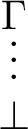
Suppose $\alpha$ is provable from $\Gamma$ in NQ:

We then show that $\Gamma \vdash \alpha$ is provable in GOM by induction on n, the number of rules applied.

• Case $n=1$. The only rule applied is Assumption rule, that is,

  $$\begin{aligned} \mathrm{a}:\alpha \end{aligned}$$

  Then, $\alpha \vdash \alpha$ is provable in GOM. Indeed,

  

  is a proof in GOM.

• Case $n > 1$. We proceed by case analysis on the last rule applied.

  • Case $\bot$-rule. By the induction hypothesis, $\Gamma \vdash \beta \wedge \lnot \beta$ is provable in GOM. Then, $\Gamma \vdash \alpha$ is provable in GOM. Indeed,

    

    is a proof in GOM.

  • Case $\mathrm{\wedge El}$-rule. By the induction hypothesis, $\alpha , \Gamma _1 \vdash \gamma$ and $\Gamma _2 \vdash \alpha \wedge \beta$ are provable in GOM. Then, $\Gamma _1, \Gamma _2 \vdash \gamma$ is provable in GOM. Indeed,

    

    is a proof in GOM.

  • Case $\mathrm{\wedge Er}$-rule. Similar to Case $\mathrm{\wedge El}$-rule.

  • Case $\mathrm{\wedge I}$-rule. By the induction hypothesis, $\Gamma _1 \vdash \alpha$ and $\Gamma _2 \vdash \beta$ are provable in GOM. Then, $\Gamma _1, \Gamma _2 \vdash \alpha \wedge \beta$ is provable in GOM:

    

  • Case $\mathrm{\rightarrow E}$-rule. By the induction hypothesis, $\Gamma _1 \vdash \alpha \rightarrow \beta$ and $\Gamma _2 \vdash \alpha$ are provable in GOM. Then, $\Gamma _1, \Gamma _2 \vdash \beta$ is provable in GOM:

    

  • Case $\mathrm{\rightarrow I}$-rule. By the induction hypothesis, $\alpha \vdash \beta$ is provable in GOM. Then, $\vdash \alpha \rightarrow \beta$ is provable in GOM:

    

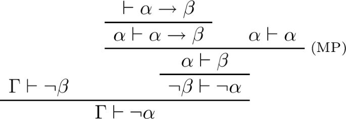
  • Case MT. By the induction hypothesis, $\vdash \alpha \rightarrow \beta$ and $\Gamma \vdash \lnot \beta$ are provable in GOM. Then, $\Gamma \vdash \lnot \alpha$ is provable in GOM:

    

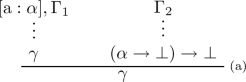
  • Case $\mathrm{\lnot \lnot I}$-rule. By the induction hypothesis, $\alpha , \Gamma \vdash \gamma$ is provable in GOM. Then, $\lnot \lnot \alpha , \Gamma \vdash \gamma$ is provable in GOM:

    

  • Case $\mathrm{\lnot \lnot E}$-rule. By the induction hypothesis, $\Gamma \vdash \alpha$ is provable in GOM. Then, $\Gamma \vdash \lnot \lnot \alpha$ is provable in GOM:

    

    $\square$

Theorem 3.6

(Admissibility of the axioms and rules of GOM in NQ). The axioms and the rules of GOM are provable in NQ.

Proof

We say that a sequent $\Gamma \vdash \Delta$ is normal if $\Delta$ consists of at most one formula. Then, the following holds (Theorem 2.5.a in [13]): If $\Gamma \vdash \Delta$ is provable in GOM, then there exists a proof of $\Gamma \vdash \Delta '$ for some $\Delta ' \subseteq \Delta$ and all the sequents occurring in that proof are normal. Using this theorem, we may only consider normal sequents. Suppose $\Gamma \vdash \Delta$ is normal and provable in GOM. Then, letting $\alpha$ be

$$\begin{aligned}{\left\{ \begin{array}{ll} \text {the single formula in } \Delta \text { if } \Delta \not \equiv \emptyset \\ \bot \text { if } \Delta \equiv \emptyset \end{array}\right. } \end{aligned}$$

we show that $\alpha$ is provable from $\Gamma$ in NQ:

by induction on n, the number of rules applied.

• Case $n = 0$. The proof is of the form:

  

  Then, $\alpha$ is provable from $\{\alpha \}$ in NQ:

  

  where $\mathrm{a}$ is arbitrarily chosen.

• Case $n > 0$. We proceed by case analysis on the last rule applied.

  • Case extension. First, we consider the case where the succedent is weakened:

    

    By the induction hypothesis, $\bot$ is provable from $\Gamma$ in NQ:

    

    Then, $\alpha$ is provable from $\Gamma$ in NQ:

    

    Second, we consider the case where the antecedent is weakened:

    

    where $\Pi \not \equiv \emptyset$. By the induction hypothesis, $\gamma$ is provable from $\Gamma$ in NQ:

    

    where $\gamma$ is either the single formula in $\Delta$, or $\bot$. Let $\Pi \equiv \{ \delta _1, \delta _2, \dots , \delta _n \}$. By applying $\mathrm{\wedge I}$-rule and $\mathrm{\wedge El}$-rule alternately:

    

    we finally observe that $\delta _1$ is provable from $\Pi$ in NQ:

    

    Then, $\gamma$ is provable from $\Gamma \cup \Pi$ in NQ:

    

    We omit the other cases where both/neither the succedent and/nor the antecedent are weakened.

  • Case cut. By the induction hypothesis, $\alpha$ is provable from $\Gamma _1$ in NQ:

    

    and $\gamma$ is provable from $\{\alpha \} \cup \Gamma _2$ in NQ:

    

    Then, $\gamma$ is provable from $\Gamma _1 \cup \Gamma _2$ in NQ:

    

  • Case $\mathrm{\wedge l_1}$. By the induction hypothesis, $\gamma$ is provable from $\{\alpha \} \cup \Gamma$ in NQ:

    

    Then, $\gamma$ is provable from $\Gamma \cup \{\alpha \wedge \beta \}$ in NQ:

    

  • Case $\mathrm{\wedge l_2}$. Similar to Case $\mathrm{\wedge l_1}$.

  • Case $\mathrm{\wedge r}$. By the induction hypothesis, $\alpha$ is provable from $\Gamma$ in NQ:

    

    and $\beta$ is provable from $\Gamma$ in NQ:

    

    Then, $\alpha \wedge \beta$ is provable from $\Gamma$ in NQ:

    

  • Case $\mathrm{\lnot l}$. By the induction hypothesis, $\alpha$ is provable from $\Gamma$ in NQ:

    

    Then, $\bot$ is provable from $\{\alpha \rightarrow \bot \} \cup \Gamma$ in NQ:

    

  • Case $\mathrm{\lnot r}$. By the induction hypothesis, $\gamma$ is provable from $\{\alpha \}$ in NQ:

    

    Then, $\alpha \rightarrow \bot$ is provable from $\{\gamma \rightarrow \bot \}$ in NQ:

    

  • Case $\mathrm{\lnot \lnot l}$. By the induction hypothesis, $\gamma$ is provable from $\{\alpha \} \cup \Gamma$ in NQ:

    

    Then, $\gamma$ is provable from $\{(\alpha \rightarrow \bot ) \rightarrow \bot \} \cup \Gamma$ in NQ:

    

  • Case $\mathrm{\lnot \lnot r}$. By the induction hypothesis, $\alpha$ is provable from $\Gamma$ in NQ:

    

    Then, $(\alpha \rightarrow \bot ) \rightarrow \bot$ is provable from $\Gamma$ in NQ:

    

  • Case O-modular. By Proposition 3.2, O-modular can be replaced by MP. By the induction hypothesis, $\alpha \rightarrow \beta$ is provable from $\Gamma$ in NQ:

    

    and $\alpha$ is provable from $\Gamma$ in NQ:

    

    Then, $\beta$ is provable from $\Gamma$ in NQ:

    

    $\square$

4 Quantum $\lambda$-Calculus

This section introduces the corresponding quantum $\lambda$-calculus together with the Curry–Howard isomorphism from NQ: the proofs of NQ can be expressed as the typed $\lambda$-terms, and vice versa (Theorem 4.7). To begin with, we construct types over a countable set of type variables and a type constant $\bot$.

Definition 4.1

(Type). Types of $\lambda$-terms are inductively defined as follows:

• $\alpha$ is a type of rank 0 if $\alpha$ is a type variable.

• $\alpha$ is a type of rank 0 if $\alpha$ is $\bot$.

• $(\alpha \times \beta )$ is a type of rank $m+n+1$ if $\alpha$ and $\beta$ are types of rank m and n, respectively.

• $(\alpha \rightarrow \beta )$ is a type of rank $m+n+1$ if $\alpha$ and $\beta$ are types of rank m and n, respectively.

• Only strings obtained by finitely many applications of the above rules are types.

Parentheses are omitted if there is no ambiguity. The rank of $\alpha$ is written as $\mathbf{rank}(\alpha )$.

Next, we construct $\lambda$-terms over a countable set of term variables.

Definition 4.2

(Typed Variable). For a term variable x and a type $\alpha$, $x:\alpha$ is said to be a typed variable.

Definition 4.3

(Environment). A finite (possibly empty) set of typed variable is said to be an environment, and is denoted by the upper-case Greek letters $\Gamma , \Delta , \Pi , \Sigma$ and those with subscripts like $\Gamma _1, \Gamma _2, \dots$.

Definition 4.4

($\textit{Typed } \lambda \textit{-Term}$). Typed $\lambda$-terms (or simply $\lambda$-terms), are inductively defined as follows:

• $x:\alpha$ is a $\lambda$-term under $\Gamma$ if $x:\alpha \in \Gamma$.

• $\varepsilon (M):\alpha$ is a $\lambda$-term under $\Gamma$ if $M:\bot$ is a $\lambda$-term under $\Gamma$ ($\alpha$ is an arbitrary type).

• $\pi _1(M):\alpha$ and $\pi _2(M):\beta$ are $\lambda$-terms under $\Gamma$ if $M:\alpha \times \beta$ is a $\lambda$-term under $\Gamma$.

• $\langle M,N \rangle : \alpha \times \beta$ is a $\lambda$-term under $\Gamma _1 \cup \Gamma _2$ if $M:\alpha$ is a $\lambda$-term under $\Gamma _1$ and $N:\beta$ is a $\lambda$-term under $\Gamma _2$, where the set of typed free variables occurring in M and N are consistent, that is, different types are not assigned to the same variables.

• $(\lambda x.M):\alpha \rightarrow \beta$ is a $\lambda$-term under $\Gamma$ if $M:\beta$ is a $\lambda$-term under $\{x:\alpha \}$, where the set of typed free variables occurring in M and $\{x:\alpha \}$ are consistent.

• $(MN):\beta$ is a $\lambda$-term under $\Gamma _1 \cup \Gamma _2$ if $M:\alpha \rightarrow \beta$ is a $\lambda$-term under $\Gamma _1$ and $N:\alpha$ is a $\lambda$-term under $\Gamma _2$.

• $\tau (M,N):\alpha \rightarrow \bot$ is a $\lambda$-term under $\Gamma$ if $M:\alpha \rightarrow \beta$ is a $\lambda$-term under $\emptyset$ and $N:\beta \rightarrow \bot$ is a $\lambda$-term under $\Gamma$.

• $\eta (M):\alpha$ is a $\lambda$-term under $\Gamma$ if $M: (\alpha \rightarrow \bot ) \rightarrow \bot$ is a $\lambda$-term under $\Gamma$.

• $\theta (M):(\alpha \rightarrow \bot ) \rightarrow \bot$ is a $\lambda$-term under $\Gamma$ if $M:\alpha$ is a $\lambda$-term under $\Gamma$.

• Only strings obtained by finitely many applications of the above rules are $\lambda$-terms.

Parentheses are omitted if there is no ambiguity; types and environments may be omitted if there is no need to specify them.

Definition 4.5

(Subterm). Let M be a $\lambda$-term. N is said to be a subterm of M if N is a substring of M and N itself is a $\lambda$-term.

Theorem 4.6

(Curry–Howard isomorphism between the formulas and the types). There exists an isomorphism between the formulas of NQ and the types of the quantum $\lambda$-calculus.

Proof

Let $\mathbf{PropVar}$ be the set of all propositional variables, and let $\mathbf{TypeVar}$ be the set of all type variables. Recall that both sets are countable. Then, there exists an isomorphism $\Phi : \mathbf{PropVar} \rightarrow \mathbf{TypeVar}$ and its reverse map $\Phi ^{-1}: \mathbf{TypeVar} \rightarrow \mathbf{PropVar}$. Let $\mathbf{Form}$ be the set of all formulas, and let $\mathbf{Type}$ be the set of all types. Then, $\Phi$ and $\Phi ^{-1}$ can be extended to an isomorphism between Form and Type as follows:

• $\Phi (\bot ) := \bot$

• $\Phi (\alpha \wedge \beta ) := \Phi (\alpha ) \times \Phi (\beta )$

• $\Phi (\alpha \rightarrow \beta ) := \Phi (\alpha ) \rightarrow \Phi (\beta )$

• $\Phi ^{-1}(\bot ) := \bot$

• $\Phi ^{-1}(\alpha \times \beta ) := \Phi ^{-1}(\alpha ) \wedge \Phi ^{-1}(\beta )$

• $\Phi ^{-1}(\alpha \rightarrow \beta ) := \Phi ^{-1}(\alpha ) \rightarrow \Phi ^{-1}(\beta )$ $\square$

Theorem 4.7

(Curry–Howard isomorphism between the proofs and the terms). There exists an isomorphism between the proofs of NQ and the $\lambda$-terms of the quantum $\lambda$-calculus.

Proof

Let $\mathbf{Label}$ be the set of all labels. Recall that this set is also countable. Then, there exists an isomorphism $\Psi : \mathbf{Label} \rightarrow \mathbf{TypeVar}$ and its reverse map $\Psi ^{-1}: \mathbf{TypeVar} \rightarrow \mathbf{Label}$. Let $\mathbf{Proof}$ be the set of all proofs, and let $\mathbf{Term}$ be the set of all $\lambda$-terms. Then, $\Psi$ and $\Psi ^{-1}$ can be extended to an isomorphism between Proof and Term as follows:

• $\Psi (\mathbf{ASM}(\mathrm{a}:\alpha /\alpha )) = \Psi (\mathrm{a}):\Phi (\alpha )$

• $\Psi (\mathbf{EFQ}(P/\alpha )) = \varepsilon (\Psi (P)):\Phi (\alpha )$

• $\Psi (\mathbf{\wedge El}(P/\alpha )) = \pi _1(\Psi (P)):\Phi (\alpha )$

• $\Psi (\mathbf{\wedge Er}(P/\beta )) = \pi _2(\Psi (P)):\Phi (\beta )$

• $\Psi (\mathbf{\wedge I}(P_1, P_2/\alpha \wedge \beta )) =\langle \Psi (P_1), \Psi (P_2)\rangle :\Phi (\alpha ) \times \Phi (\beta )$

• $\Psi (\mathbf{\rightarrow E}(P_1, P_2/\beta )) = (\Psi (P_1)\Psi (P_2)):\Phi (\beta )$

• $\Psi (\mathbf{\rightarrow I}(P[\mathrm{a}:\alpha ]/\alpha \rightarrow \beta )) = \lambda \Psi (\mathrm{a}).\Psi (P):\Phi (\alpha ) \rightarrow \Phi (\beta )$

• $\Psi (\mathbf{MT}(P_1, P_2/\alpha \rightarrow \bot )) = \tau (\Psi (P_1),\Psi (P_2)):\Phi (\alpha )\rightarrow \bot$

• $\Psi (\mathbf{\lnot \lnot E}(P/\alpha )) = \eta (\Psi (P)):\Phi (\alpha )$

• $\Psi (\mathbf{\lnot \lnot I}(P/\alpha \rightarrow \bot )) = \theta (\Psi (P)):(\Phi (\alpha ) \rightarrow \bot ) \rightarrow \bot$

• $\Psi ^{-1}(x:\alpha ) = \mathbf{ASM}(\Psi ^{-1}(x):\Phi ^{-1}(\alpha )/\Phi ^{-1}(\alpha ))$

• $\Psi ^{-1}(\varepsilon (M:\bot ):\alpha ) = \mathbf{EFQ}(\Psi ^{-1}(M:\bot )/\Phi ^{-1}(\alpha ))$

• $\Psi ^{-1}(\pi _1(M:\alpha \times \beta ):\alpha ) = \mathbf{\wedge El}(\Psi ^{-1}(M:\alpha \times \beta )/\Phi ^{-1}(\alpha ))$

• $\Psi ^{-1}(\pi _2(M:\alpha \times \beta ):\beta ) = \mathbf{\wedge Er}(\Psi ^{-1}(M:\alpha \times \beta )/\Phi ^{-1}(\beta ))$

• $\Psi ^{-1}(\langle M:\alpha , N:\beta \rangle :\alpha \times \beta ) = \mathbf{\wedge I}(\Psi ^{-1}(M:\alpha ), \Psi ^{-1}(N:\beta )/\Phi ^{-1}(\alpha ) \wedge \Phi ^{-1}(\beta ))$

• $\Psi ^{-1}(((M:\alpha \rightarrow \beta )(N:\beta )):\beta ) = \mathbf{\rightarrow E}(\Psi ^{-1}(M:\alpha \rightarrow \beta ), \Psi ^{-1}(N:\alpha )/\Phi ^{-1}(\beta ))$

• $\Psi ^{-1}(\lambda x.(M:\beta ):\alpha \rightarrow \beta ) = \mathbf{\rightarrow I}(\Psi ^{-1}(M:\beta )[\Psi ^{-1}(x):\Phi ^{-1}(\alpha )] /\Phi ^{-1}(\alpha ) \rightarrow \Phi ^{-1}(\beta ))$

• $\Psi ^{-1}(\tau ((M:\alpha \rightarrow \bot ),(N:\beta \rightarrow \bot )):\alpha \rightarrow \bot ) = \mathbf{MT}(\Psi ^{-1}(M:\alpha \rightarrow \beta ), \Psi ^{-1}(N:\beta \rightarrow \bot )/\Phi ^{-1}(\alpha ) \rightarrow \bot )$

• $\Psi ^{-1}(\eta (M:(\alpha \rightarrow \bot )\rightarrow \bot )):\alpha ) = \mathbf{\lnot \lnot E}(\Psi ^{-1}(M:(\alpha \rightarrow \bot ) \rightarrow \bot )/\Phi ^{-1}(\alpha ))$

• $\Psi ^{-1}(\theta (M:\alpha ):(\alpha \rightarrow \bot )\rightarrow \bot ){=}{} \mathbf{\lnot \lnot I}(\Psi ^{-1}(M:\alpha )/(\Phi ^{-1}(\alpha ) \rightarrow \bot ) \rightarrow \bot )$ $\square$

Definition 4.8

(Conversion). A $\lambda$-term M is said to be converted if a subterm of M is substituted with another $\lambda$-term in the following way:

• $\pi _1(\langle N:\alpha , L:\beta \rangle )$ is substituted with $N:\alpha$. In NQ, a section of a proof:

  

  is converted to

  

• $\pi _2(\langle N:\alpha , L:\beta \rangle )$ is substituted with $L:\beta$. In NQ, a section of a proof:

  

  is converted to

  

• $(\lambda x:\alpha .N:\beta )(L:\alpha )$ is converted to $(N[x:=L:\alpha ]):\beta$. Here, $N[x:=L]$ represents the substitution instance of N where all the free occurrences of x are substituted with L. The bound variables are assumed to have been renamed consistently, in order to avoid capturing free variables. In NQ, a section of a proof:

  

  is converted to

  

• $\eta (\theta (M:\alpha ))$ is converted to $M:\alpha$. In NQ, a section of a proof:

  

  is converted to

  

Henceforth, we write $M \Rightarrow M'$ to mean that M is converted to $M'$ in one step. Note that converting a $\lambda$-term can be seen as executing a computation, while converting a proof can be seen as removing a detour in it. A conversion sequence $M_0 \Rightarrow M_1 \Rightarrow \cdots \Rightarrow M_n$ of $\lambda$-terms (or $P_0 \Rightarrow P_1 \Rightarrow \cdots \Rightarrow P_n$ of proofs) is denoted by $M_0 \Rightarrow ^* M_n$ ($P_0 \Rightarrow ^* P_n$). Here, $n \ge 0$, that is, $\Rightarrow ^*$ includes the possibility that no conversion is performed.

Definition 4.9

(Normal form). A $\lambda$-term (or a proof) is said to be in its normal form if it cannot be further converted. A $\lambda$-term is said to be normalizable if there exists a conversion sequence that starts with itself and ends with its normal form.

5 Strong Normalization

This section establishes a rigorous proof of the strong normalization property for the quantum $\lambda$-calculus (Theorem 5.2).

Definition 5.1

(Strongly normalizing). A $\lambda$-term is said to be strongly normalizing if there exists no infinite conversion sequence that starts with itself.

Theorem 5.2

(Strong normalization). The $\lambda$-terms of the quantum $\lambda$-calculus are strongly normalizing.

To prove this theorem, we need some preliminaries. Let $\mathbf{Term}$ be the set of all $\lambda$-terms, and let $\mathbf{SNTerm}$ be the set of all strongly normalizing $\lambda$-terms. For $M \in \mathbf{SNTerm}$, the maximum length of a conversion sequence that starts with M is written as |M|.

Definition 5.3

($\mathbf{RED}_\alpha$). For each type $\alpha$, a set $\mathbf{RED}_\alpha$ of $\lambda$-terms is inductively defined as follows:

• Case $\mathbf{rank}(\alpha ) = 0$. $\mathbf{RED}_\alpha$ is $\mathbf{SNTerm}$. In particular, $\mathbf{RED}_\bot$ is $\mathbf{SNTerm}$.

• Case $\mathbf{rank}(\alpha ) > 0$.

  • Case $\alpha \equiv \beta \times \gamma$. $\mathbf{RED}_{\beta \times \gamma }$ is the set of all those $\lambda$-terms M that satisfy the following condition: $\pi _1(M) \in \mathbf{RED}_{\beta }$ and $\pi _2(M) \in \mathbf{RED}_{\gamma }$.

  • Case $\alpha \equiv \beta \rightarrow \gamma$. $\mathbf{RED}_{\beta \rightarrow \gamma }$ is the set of all those $\lambda$-terms M that satisfy the following conditions:

    • (a) $MN \in \mathbf{RED}_\gamma$ for any $N \in \mathbf{RED}_\beta$.

    • (b) $\eta (M) \in \mathbf{RED}_\delta$ if $\beta \equiv \delta \rightarrow \gamma$.

Proposition 5.4

For each type $\alpha$, $\mathbf{RED}_\alpha$ satisfies the following conditions:

• (C1) $\mathbf{RED}_\alpha \subseteq \mathbf{SNTerm}$.

• (C2) If $M \in \mathbf{RED}_\alpha$ and $M \Rightarrow ^* M'$, then $M' \in \mathbf{RED}_\alpha$.

• (C3) If M is of the form other than $N \times L$ (product), $\lambda x.N$ ($\lambda$-abstraction), or $\theta (N)$ (double-negation), and if $M' \in \mathbf{RED}_\alpha$ for any $M'$ with $M \Rightarrow M'$, then $M \in \mathbf{RED}_\alpha$.

Note that (C3) implies the following: if M is of the form other than product, $\lambda$-abstraction, or double-negation, and if M is in its normal form, then $M \in \mathbf{RED}_\alpha$ for any $\alpha$.

Proof

By induction on $\mathbf{rank}(\alpha )$.

• Case $\mathbf{rank}(\alpha ) = 0$. By definition, $\mathbf{RED}_\alpha$ is $\mathbf{SNTerm}$.

  • (C1) Immediate.

  • (C2) Suppose $M \in \mathbf{SNTerm}$ and $M \Rightarrow ^* M'$. Then, it is immediate that $M' \in \mathbf{SNTerm}$.

  • (C3) Suppose $M \Rightarrow M'$ and $M' \in \mathbf{RED}_\alpha$ ($= \mathbf{SNTerm}$). Letting $m := \max \{ |M'| \mid M \Rightarrow M' \}$, we have $|M| = m + 1$. Hence $M \in \mathbf{SNTerm}$.

• Case $\mathbf{rank}(\alpha ) > 0$. We proceed by case analysis on the form of $\alpha$.

  • Case $\alpha \equiv \beta \times \gamma$.

    • (C1) Suppose $M \in \mathbf{RED}_{\beta \times \gamma }$. We will show $M \in \mathbf{SNTerm}$. From the assumption that $M \in \mathbf{RED}_{\beta \times \gamma }$, it follows that $\pi _1 (M) \in \mathbf{RED}_\beta$. Then, by the induction hypothesis (C1), we have $\pi _1 (M) \in \mathbf{SNTerm}$. Applying $\pi _1$ to a conversion sequence that starts with M, say $M \Rightarrow M_1 \Rightarrow M_2 \Rightarrow \dots$, we get the sequence $\pi _1 (M) \Rightarrow \pi _1 (M_1) \Rightarrow \pi _1 (M_2) \Rightarrow \dots$, which means that $|M| \le |\pi _1 (M)|$. Hence, we have $M \in \mathbf{SNTerm}$.

    • (C2) Suppose that $M \in \mathbf{RED}_{\beta \times \gamma }$ and $M \Rightarrow ^* M'$. We will show $M' \in \mathbf{RED}_{\beta \times \gamma }$. From the assumption that $M \in \mathbf{RED}_{\beta \times \gamma }$, it follows that $\pi _1 (M) \in \mathbf{RED}_\beta$ and $\pi _2 (M) \in \mathbf{RED}_\gamma$. Moreover, from the assumption that $M \Rightarrow ^* M'$, it follows that $\pi _1 (M) \Rightarrow ^* \pi _1 (M')$ and $\pi _2 (M) \Rightarrow ^* \pi _2 (M')$. Then, by the induction hypothesis (C2), we have that $\pi _1 (M') \in \mathbf{RED}_\beta$ and $\pi _2 (M') \in \mathbf{RED}_\gamma$. Hence, by the definition of $\mathbf{RED}_{\beta \times \gamma }$, we have $M' \in \mathbf{RED}_{\beta \times \gamma }$.

    • (C3) Suppose that M is of the form other than product, $\lambda$-abstrac- tion, or double-negation, and suppose $M' \in \mathbf{RED}_\alpha$ for any $M'$ with $M \Rightarrow M'$. We will show $M \in \mathbf{RED}_{\beta \times \gamma }$. Since M is of the form other than product, the possible one-step conversion from $\pi _1 (M)$ is of the form $\pi _1 (M) \Rightarrow \pi _1 (M')$ with $M \Rightarrow M'$. From the assumption that $M' \in \mathbf{RED}_{\beta \times \gamma }$, it follows that $\pi _1 (M') \in \mathbf{RED}_\beta$. Then, by the induction hypothesis (C3), we have $\pi _1 (M) \in \mathbf{RED}_\beta$. Similarly, $\pi _2 (M) \in \mathbf{RED}_\gamma$. Hence, by the definition of $\mathbf{RED}_{\beta \times \gamma }$, we have $M \in \mathbf{RED}_{\beta \times \gamma }$.

  • Case $\alpha \equiv \beta \rightarrow \gamma$.

    • (C1) Suppose $M \in \mathbf{RED}_{\beta \rightarrow \gamma }$. We will show $M \in \mathbf{SNterm}$. From the assumption that $M \in \mathbf{RED}_{\beta \rightarrow \gamma }$, it follows that:

      • (a) $MN \in \mathbf{RED}_\gamma$ for any $N \in \mathbf{RED}_\beta$.

      • (b) $\eta (M) \in \mathbf{RED}_\delta$ if $\beta \equiv \delta \rightarrow \gamma$.

      Let $x:\beta$ be a typed variable. Note that x is in its normal form. Then, by the induction hypothesis (C3), we have $x \in \mathbf{RED}_\beta$. Hence, by (a), we have $Mx \in \mathbf{RED}_\gamma$. Then, by the induction hypothesis (C1), we have $Mx \in \mathbf{SNTerm}$. Applying a conversion sequence that starts with M, say $M \Rightarrow M_1 \Rightarrow M_2 \Rightarrow \dots$, to x, we get the sequence $Mx \Rightarrow M_1 x \Rightarrow M_2 x \Rightarrow \dots$, which means that $|M| \le |Mx|$. Hence, we have $M \in \mathbf{SNTerm}$.

    • (C2) Suppose that $M \in \mathbf{RED}_{\beta \rightarrow \gamma }$ and $M \Rightarrow ^* M'$. We will show $M' \in \mathbf{RED}_{\beta \rightarrow \gamma }$. To show this, we need to verify:

      • (a) $M'N \in \mathbf{RED}_\gamma$ for any $N \in \mathbf{RED}_\beta$.

      • (b) $\eta (M') \in \mathbf{RED}_\delta$ if $\beta \equiv \delta \rightarrow \gamma$.

      For (a): From the assumption that $M \in \mathbf{RED}_{\beta \rightarrow \gamma }$, it follows that $MN \in \mathbf{RED}_\gamma$ for any $N \in \mathbf{RED}_\beta$. Moreover, from the assumption that $M \Rightarrow ^* M'$, it follows that $MN \Rightarrow ^* M'N$. Then, by the induction hypothesis (C2), we have $M'N \in \mathbf{RED}_\gamma$. For (b): Let $\beta \equiv \delta \rightarrow \gamma$. From the assumption that $M \in \mathbf{RED}_{\beta \rightarrow \gamma }$, it follows that $\eta (M) \in \mathbf{RED}_\delta$. Moreover, from the assumption that $M \Rightarrow ^* M'$, it follows that $\eta (M) \Rightarrow ^* \eta (M')$. Then, by the induction hypothesis (C2), we have $\eta (M') \in \mathbf{RED}_\delta$.

    • (C3) Suppose that M is of the form other than product, $\lambda$-abstrac- tion, or double-negation, and suppose $M' \in \mathbf{RED}_{\beta \rightarrow \gamma }$ for any $M'$ with $M \Rightarrow M'$. We will show $M \in \mathbf{RED}_{\beta \rightarrow \gamma }$. To show this, we need to verify:

      • (a) $MN \in \mathbf{RED}_\gamma$ for any $N \in \mathbf{RED}_\beta$.

      • (b) $\eta (M) \in \mathbf{RED}_\delta$ if $\beta \equiv \delta \rightarrow \gamma$.

      For (a): Suppose $N \in \mathbf{RED}_\beta$. Note that by the induction hypothesis (C1), we have $N \in \mathbf{SNTerm}$. Then, we can show $MN \in \mathbf{RED}_\gamma$ by induction on |N|:

      • Case $|N| = 0$. Suppose $MN \Rightarrow L$. Since N is in its normal form, the possible form of L is $L \equiv M'N$ with $M \Rightarrow M'$. From the assumption that $M' \in \mathbf{RED}_{\beta \rightarrow \gamma }$, it follows that $M'N \in \mathbf{RED}_\gamma$. Then, by the induction hypothesis (C3), we have $MN \in \mathbf{RED}_\gamma$.

      • Case $|N| > 0$. Suppose $MN \Rightarrow L$. Since M is of the form other than $\lambda$-abstraction, the possible forms of L are the following:

        • Case $L \equiv M'N$ with $M \Rightarrow M'$. Then, we have $MN \in \mathbf{RED}_\gamma$ as described above.

        • Case $L \equiv MN'$ with $N \Rightarrow N'$. By the hypothesis (C2) of the induction on $\mathbf{rank}(\alpha )$, we have $N' \in \mathbf{RED}_\beta$. Note that $|N'| = |N| - 1 < |N|$. Then, by the hypothesis of the induction on |N|, we have $MN' \in \mathbf{RED}_\gamma$.

        Thus, by the hypothesis (C3) of the induction on $\mathbf{rank}(\alpha )$, we have $MN \in \mathbf{RED}_\gamma$.

      For (b): Let $\beta \equiv \delta \rightarrow \gamma$. Since M is of the form other than double-negation, the possible one-step conversion that starts with $\eta (M)$ is of the form $\eta (M) \Rightarrow \eta (M')$ with $M \Rightarrow M'$. From the assumption that $M' \in \mathbf{RED}_{\beta \rightarrow \gamma }$, it follows that $\eta (M') \in \mathbf{RED}_\delta$. Then, by the induction hypothesis (C3), we have $\eta (M) \in \mathbf{RED}_\delta$.$\square$

Proposition 5.5

The followings hold:

• 1. If $M \in \mathbf{RED}_\bot$, then $\varepsilon (M) \in \mathbf{RED}_\alpha$ for any $\alpha$.

• 2. If $M \in \mathbf{RED}_\alpha$ and $N \in \mathbf{RED}_\beta$, then $\langle M, N \rangle \in \mathbf{RED}_{\alpha \times \beta }$.

• 3. If $M[x:=N] \in \mathbf{RED}_\beta$ for any $N \in \mathbf{RED}_\alpha$, then $\lambda x.M \in \mathbf{RED}_{\alpha \rightarrow \beta }$.

• 4. If $M \in \mathbf{RED}_{\alpha \rightarrow \beta }$ and $N \in \mathbf{RED}_{\beta \rightarrow \bot }$, then $\tau (M,N) \in \mathbf{RED}_{\alpha \rightarrow \bot }$.

• 5. If $M \in \mathbf{RED}_\alpha$, then $\theta (M) \in \mathbf{RED}_{(\alpha \rightarrow \bot ) \rightarrow \bot }$.

Proof

• 1. Suppose $M \in \mathbf{RED}_\bot$ ($= \mathbf{SNTerm}$). We will show $\varepsilon (M) \in \mathbf{RED}_\alpha$ by induction on $\mathbf{rank}(\alpha )$.

  • Case $\mathbf{rank}(\alpha ) = 0$. From the assumption that $M \in \mathbf{SNTerm}$, it follows that any conversion sequence that starts with M is finite. Then, any sequence starts with $\varepsilon (M)$ is also finite. Hence, we have $\varepsilon (M) \in \mathbf{SNTerm} = \mathbf{RED}_\alpha$.

  • Case $\mathbf{rank}(\alpha ) > 0$. We will show $\varepsilon (M) \in \mathbf{RED}_\alpha$ by induction on |M|.

    • Case $|M| = 0$. Note that M is in its normal form, and so is $\varepsilon (M)$. Hence, by (C3), we have $\varepsilon (M) \in \mathbf{RED}_\alpha$.

    • Case $|M| > 0$. Suppose $\varepsilon (M) \Rightarrow L$. The possible form of L is $L \equiv \varepsilon (M')$ with $M \Rightarrow M'$. From the assumption that $M \in \mathbf{RED}_\bot$ and (C2) , we have $M' \in \mathbf{RED}_\bot$. Note that $|M'| = |M| - 1 < |M|$. Then, by the hypothesis of the induction on |M|, we have $L \in \mathbf{RED}_\alpha$. Hence, by (C3), we have $\varepsilon (M) \in \mathbf{RED}_\alpha$.

• 2. Suppose that $M \in \mathbf{RED}_\alpha$ and $N \in \mathbf{RED}_\beta$. We will show $\pi _1 (\langle M, N \rangle ) \in \mathbf{RED}_\alpha$ by induction on $|M| + |N|$.

  • Case $|M| + |N| = 0$. Suppose $\pi _1 (\langle M, N\rangle ) \Rightarrow L$. Since M and N are in their normal forms, the possible form of L is $L \equiv M$. From the assumption that $M \in \mathbf{RED}_\alpha$, we have $L \in \mathbf{RED}_\alpha$. Hence, by (C3), we have $\pi _1 (\langle M, N\rangle ) \in \mathbf{RED}_\alpha$.

  • Case $|M| + |N| > 0$. Suppose $\pi _1 (\langle M, N\rangle ) \Rightarrow L$. The possible forms of L are the following:

    • Case $L \equiv \pi _1 (\langle M', N\rangle )$ with $M \Rightarrow M'$. From the assumption that $M \in \mathbf{RED}_\alpha$ and (C2), it follows that $M' \in \mathbf{RED}_\alpha$. Note that $|M'| = |M| - 1 < |M|$. Then, by the hypothesis of the induction on $|M| + |N|$, we have $L \in \mathbf{RED}_\alpha$.

    • Case $L \equiv \pi _1 (\langle M, N'\rangle )$ with $N \Rightarrow N'$. From the assumption that $N \in \mathbf{RED}_\beta$ and (C2), it follows that $N' \in \mathbf{RED}_\beta$. Note that $|N'| = |N| - 1 < |N|$. Then, by the hypothesis of the induction on $|M| + |N|$, we have $L \in \mathbf{RED}_\alpha$.

    • Case $L \equiv M$. From the assumption that $M \in \mathbf{RED}_\alpha$, it follows that $L \in \mathbf{RED}_\alpha$.

    Hence, by (C3), we have $\pi _1 (\langle M, N\rangle ) \in \mathbf{RED}_\alpha$.

  Similarly, $\pi _2 (\langle M, N\rangle ) \in \mathbf{RED}_\beta$. Hence, we have $\langle M, N\rangle \in \mathbf{RED}_{\alpha \times \beta }$.

• 3. Suppose $M[x:=N] \in \mathbf{RED}_\beta$ for any $N \in \mathbf{RED}_\alpha$. We will show $\lambda x.M \in \mathbf{RED}_{\alpha \rightarrow \beta }$. To show this, we need to verify:

  • (a) $(\lambda x.M)N \in \mathbf{RED}_\beta$ for any $N \in \mathbf{RED}_\alpha$.

  • (b) $\eta (\lambda x.M) \in \mathbf{RED}_\gamma$ if $\alpha \equiv \gamma \rightarrow \beta$.

  For (a): Suppose $N \in \mathbf{RED}_\alpha$. We will show $(\lambda x.M)N \in \mathbf{RED}_\beta$ by induction on $|M| + |N|$.

  • Case $|M| + |N| = 0$. Suppose $(\lambda x.M)N \Rightarrow L$. Since M and N are in their normal forms, the possible form of L is $L \equiv M[x:=N]$. From the assumption that $M[x:=N] \in \mathbf{RED}_\beta$ for any $N \in \mathbf{RED}_\alpha$, and the assumption that $N \in \mathbf{RED}_\alpha$, it follows that $L \in \mathbf{RED}_\beta$. Hence, by (C3), we have $(\lambda x.M)N \in \mathbf{RED}_\beta$.

  • Case $|M| + |N| > 0$. Suppose $(\lambda x.M)N \Rightarrow L$. The possible forms of L are the following:

    • Case $L \equiv (\lambda x.M')N$ with $M \Rightarrow M'$. From the assumption that $M[x:=N] \in \mathbf{RED}_\beta$ for any $N \in \mathbf{RED}_\alpha$, and the fact that $x \in \mathbf{RED}_\alpha$, it follows that $M \equiv M[x:=x] \in \mathbf{RED}_\beta$. Then, by (C2), we have $M' \in \mathbf{RED}_\beta$. Note that $|M'| = |M| - 1 < |M|$. Then, by the hypothesis of the induction on $|M| + |N|$, we have $L \in \mathbf{RED}_\beta$.

    • Case $L \equiv (\lambda x.M)N'$ with $N \Rightarrow N'$. From the assumption that $N \in \mathbf{RED}_\alpha$ and (C2), it follows that $N' \in \mathbf{RED}_\alpha$. Note that $|N'| = |N| - 1 < |N|$. Then, by the hypothesis of the induction on $|M| + |N|$, we have $L \in \mathbf{RED}_\beta$.

    • Case $L \equiv M[x:=N]$. From the assumption that $M[x:=N] \in \mathbf{RED}_\beta$ for any $N \in \mathbf{RED}_\alpha$ and the assumption that $N \in \mathbf{RED}_\alpha$, it follows that $L \in \mathbf{RED}_\beta$.

    Hence, by (C3), we have $(\lambda x.M)N \in \mathbf{RED}_\beta$.

  For (b): Let $\alpha \equiv \gamma \rightarrow \beta$. We will show $\eta (\lambda x.M) \in \mathbf{RED}_\gamma$ by induction on |M|.

  • Case $|M| = 0$. Note that M is in its normal form, and so is $\eta (\lambda x.M)$. Hence, by (C3), we have $\eta (\lambda x.M) \in \mathbf{RED}_\gamma$.

  • Case $|M| > 0$. Suppose $\eta (\lambda x.M) \Rightarrow L$. The possible form of L is $L \equiv \eta (\lambda x.M')$ with $M \Rightarrow M'$. Note that $|M'| = |M| - 1 < |M|$. Then, by the hypothesis of the induction on |M|, we have $\eta (\lambda x.M') \in \mathbf{RED}_\gamma$. Hence, by (C3), we have $\eta (\lambda x.M) \in \mathbf{RED}_\gamma$.

• 4. Suppose that $M \in \mathbf{RED}_{\alpha \rightarrow \beta }$ and $N \in \mathbf{RED}_{\beta \rightarrow \bot }$. We will show $\tau (M, N) \in \mathbf{RED}_{\alpha \rightarrow \bot }$ by induction on $|M| + |N|$.

  • Case $|M| + |N| = 0$. Since M and N are in their normal forms, so is $\tau (M, N)$. Then, by (C3), we have $\tau (M, N) \in \mathbf{RED}_{\alpha \rightarrow \bot }$.

  • Case $|M| + |N| > 0$. Suppose $\tau (M,N) \Rightarrow L$. The possible forms of L are the following:

    • Case $L \equiv \tau (M', N)$ with $M \Rightarrow M'$. From the assumption that $M \in \mathbf{RED}_{\alpha \rightarrow \beta }$ and (C2), it follows that $M' \in \mathbf{RED}_{\alpha \rightarrow \beta }$. Note that $|M'| = |M| - 1 < |M|$. Then, by the hypothesis of the induction on $|M| + |N|$, we have $L \in \mathbf{RED}_{\alpha \rightarrow \bot }$.

    • Case $L \equiv \tau (M, N')$ with $N \Rightarrow N'$. From the assumption that $N \in \mathbf{RED}_{\beta \rightarrow \bot }$ and (C2), it follows that $N' \in \mathbf{RED}_{\beta \rightarrow \bot }$. Note that $|N'| = |N| - 1 < |N|$. Then, by the hypothesis of the induction on $|M| + |N|$, we have $L \in \mathbf{RED}_{\alpha \rightarrow \bot }$.

    Hence, by (C3), we have $\tau (M, N) \in \mathbf{RED}_{\alpha \rightarrow \bot }$.

• 5. Suppose $M \in \mathbf{RED}_\alpha$. We will show $\theta (M) \in \mathbf{RED}_{(\alpha \rightarrow \bot ) \rightarrow \bot }$. To show this, we need to verify:

  • (a) $\theta (M)N \in \mathbf{RED}_\bot$ for any $N \in \mathbf{RED}_{\alpha \rightarrow \bot }$.

  • (b) $\eta (\theta (M)) \in \mathbf{RED}_\alpha$.

  For (a) : Suppose $N \in \mathbf{RED}_{\alpha \rightarrow \bot }$. We will show $\theta (M)N \in \mathbf{RED}_{\bot }$ by induction on $|M| + |N|$.

  • Case $|M| + |N| = 0$. Since M and N are in their normal forms, so is $\theta (M)N$. Then, by (C3), we have $\theta (M)N \in \mathbf{RED}_{\bot }$.

  • Case $|M| + |N| > 0$. Suppose $\theta (M)N \Rightarrow L$. The possible forms of L are the following:

    • Case $L \equiv \theta (M')N$ with $M \Rightarrow M'$. From the assumption that $M \in \mathbf{RED}_{\alpha }$ and (C2), it follows that $M' \in \mathbf{RED}_{\alpha }$. Note that $|M'| = |M| - 1 < |M|$. Then, by the hypothesis of the induction on $|M| + |N|$, we have $L \in \mathbf{RED}_{\bot }$.

    • Case $L \equiv \theta (M)N'$ with $N \Rightarrow N'$. From the assumption that $N \in \mathbf{RED}_{\alpha \rightarrow \bot }$ and (C2), it follows that $N' \in \mathbf{RED}_{\alpha \rightarrow \bot }$. Note that $|N'| = |N| - 1 < |N|$. Then, by the hypothesis of the induction on $|M| + |N|$, we have $L \in \mathbf{RED}_{\bot }$.

    Hence, by (C3), we have $\theta (M)N \in \mathbf{RED}_{\bot }$.

  For (b): We will show $\eta (\theta (M)) \in \mathbf{RED}_\alpha$ by induction on |M|.

  • Case $|M| = 0$. Suppose $\eta (\theta (M)) \Rightarrow L$. Since M is in its normal form, the possible form of L is $L \equiv M$. From the assumption that $M \in \mathbf{RED}_\alpha$, it follows that $L \in \mathbf{RED}_\alpha$. Hence, by (C3), we have $\eta (\theta (M)) \in \mathbf{RED}_\alpha$.

  • Case $|M| > 0$. Suppose $\eta (\theta (M)) \Rightarrow L$. The possible forms of L are the following:

    • Case $L \equiv M$. From the assumption that $M \in \mathbf{RED}_\alpha$, it follows that $L \in \mathbf{RED}_\alpha$.

    • Case $L \equiv \eta (\theta (M'))$ with $M \Rightarrow M'$. From the assumption that $M \in \mathbf{RED}_\alpha$ and (C2), it follows that $M' \in \mathbf{RED}_\alpha$. Note that $|M'| = |M| - 1 < |M|$. Then, by the hypothesis of the induction on |M|, we have $L \in \mathbf{RED}_\alpha$.

    Hence, by (C3), we have $\eta (\theta (M)) \in \mathbf{RED}_\alpha$.$\square$

Proof of Theorem 5.2

Let $M:\alpha$ be a $\lambda$-term. We will show $M \in \mathbf{RED}_\alpha$. Then, by (C1), we will have $M \in \mathbf{SNTerm}$. More generally, the following holds: If M has no free variables other than $x_1:\alpha _1, \dots , x_n:\alpha _n$, and if $M_1:\alpha _1 \in \mathbf{RED}_{\alpha _1}, \dots , M_n:\alpha _n \in \mathbf{RED}_{\alpha _n}$, then $M[x_1 := M_1, \dots , x_n := M_n] \in \mathbf{RED}_\alpha$. We will show this by induction on the construction of M.

• Case $M \equiv x_i$. Immediate.

• Case $M \equiv \varepsilon (N)$. Let $N:\bot$ be a $\lambda$-term. Suppose that N has no free variables other than $x_1:\alpha _1, \dots , x_n:\alpha _n$, and suppose $M_1:\alpha _1 \in \mathbf{RED}_{\alpha _1}, \dots , M_n:\alpha _n \in \mathbf{RED}_{\alpha _n}$. By the induction hypothesis, we have $N[x_1 := M_1, \dots , x_n := M_n ] \in \mathbf{RED}_\bot$. Then, by 1 of Proposition 5.5, we have $(\varepsilon (N))[x_1 := M_1, \dots , x_n := M_n ] \equiv \varepsilon (N[x_1 := M_1,\dots , x_n := M_n ]) \in \mathbf{RED}_\alpha$.

• Case $M \equiv \pi _1 (N)$. Let $N:\alpha \times \beta$ be a $\lambda$-term. Suppose that N has no free variables other than $x_1:\alpha _1, \cdots , x_n:\alpha _n$, and suppose $M_1:\alpha _1 \in \mathbf{RED}_{\alpha _1}, \dots , M_n:\alpha _n \in \mathbf{RED}_{\alpha _n}$. By the induction hypothesis, we have $N[x_1 := M_1, \dots , x_n := M_n ] \in \mathbf{RED}_{\alpha \times \beta }$. Then, by the definition of $\mathbf{RED}_{\alpha \times \beta }$, we have $(\pi _1(N))[x_1 := M_1, \dots , x_n := M_n ] \equiv \pi _1 (N[x_1 := M_1, \dots , x_n := M_n ]) \in \mathbf{RED}_\alpha$.

• Case $M \equiv \pi _2(N)$. Similar to Case $\pi _1(N)$.

• Case $M \equiv \langle N, L\rangle$. Let $N:\beta$ and $L:\gamma$ be $\lambda$-terms. Accordingly, $\alpha \equiv \beta \times \gamma$. Suppose that N and L have no free variables other than $x_1:\alpha _1, \dots , x_n:\alpha _n$, and suppose $M_1:\alpha _1 \in \mathbf{RED}_{\alpha _1}, \dots , M_n:\alpha _n \in \mathbf{RED}_{\alpha _n}$. By the induction hypothesis, we have $N[x_1 := M_1, \dots , x_n := M_n] \in \mathbf{RED}_\beta$ and $L[x_1 := M_1, \dots , x_n := M_n] \in \mathbf{RED}_\gamma$. Then, by 2 of Proposition 5.5, we have $\langle N, L \rangle [x_1 := M_1, \dots , x_n := M_n] \equiv \langle N[x_1 := M_1, \dots , x_n := M_n], L[x_1 := M_1,\dots , x_n := M_n]\rangle \in \mathbf{RED}_\alpha$.

• Case $M \equiv NL$. Let $N:\beta$ and $L:\gamma$ be $\lambda$-terms. Accordingly, $\beta \equiv \gamma \rightarrow \alpha$. Suppose that N and L have no free variables other than $x_1:\alpha _1, \dots , x_n:\alpha _n$, and suppose $M_1:\alpha _1\in \mathbf{RED}_{\alpha _1}, \dots , M_n:\alpha _n \in \mathbf{RED}_{\alpha _n}$. By the induction hypothesis, we have $N[x_1 := M_1, \dots , x_n := M_n] \in \mathbf{RED}_\beta$ and $L[x_1 := M_1, \dots , x_n := M_n] \in \mathbf{RED}_\gamma$. Then, by the definition of $\mathbf{RED}_{\gamma \rightarrow \alpha }$, we have $(NL)[x_1 := M_1, \dots , x_n := M_n] \equiv N[x_1 := M_1, \dots , x_n := M_n](L[x_1 := M_1, \dots , x_n := M_n]) \in \mathbf{RED}_\alpha$.

• Case $M \equiv \lambda y.N$. Let $y:\beta$ be a typed variable and let $N:\gamma$ be a $\lambda$-term. Accordingly, $\alpha \equiv \beta \rightarrow \gamma$. Suppose that N has no free variables other than $x_1:\alpha _1, \dots , x_n:\alpha _n, y:\beta$, and suppose $M_1:\alpha _1 \in \mathbf{RED}_{\alpha _1}, \dots , M_n:\alpha _n \in \mathbf{RED}_{\alpha _n}, L:\beta \in \mathbf{RED}_\beta$. By the induction hypothesis, we have $N[x_1 := M_1, \cdots , x_n := M_n, y := L] \in \mathbf{RED}_\gamma$. Then, by 3 of Proposition 5.5, we have $(\lambda y.N)[x_1 := M_1, \dots , x_n := M_n] \equiv \lambda y.(N[x_1 := M_1, \dots , x_n := M_n]) \in \mathbf{RED}_\alpha$.

• Case $M \equiv \tau (N,L)$. Let $N:\beta \rightarrow \gamma$ and $L:\gamma \rightarrow \bot$ be $\lambda$-terms. Accordingly, $\alpha \equiv \beta \rightarrow \bot$. Supose that N and L have no free variables other than $x_1:\alpha _1, \dots , x_n:\alpha _n$, and suppose $M_1:\alpha _1 \in \mathbf{RED}_{\alpha _1}, \dots , M_n:\alpha _n \in \mathbf{RED}_{\alpha _n}$. By the induction hypothesis, we have $N[x_1 := M_1, \dots , x_n := M_n] \in \mathbf{RED}_{\beta \rightarrow \gamma }$ and $L[x_1 := M_1, \dots , x_n := M_n] \in \mathbf{RED}_{\gamma \rightarrow \bot }$. Then, by 4 of Proposition 5.5, we have $\tau (N, L)[x_1 := M_1, \dots , x_n := M_n] \equiv \tau (N[x_1 := M_1, \dots , x_n := M_n], L[x_1 := M_1, \dots , x_n := M_n]) \in \mathbf{RED}_\alpha$.

• Case $M \equiv \eta (N)$. Let $N:(\alpha \rightarrow \bot ) \rightarrow \bot$ be a $\lambda$-term. Suppose that N has no free variables other than $x_1:\alpha _1, \cdots , x_n:\alpha _n$, and suppose $M_1:\alpha _1 \in \mathbf{RED}_{\alpha _1}, \dots , M_n:\alpha _n \in \mathbf{RED}_{\alpha _n}$. By the induction hypothesis, we have $N[x_1 := M_1, \dots , x_n := M_n] \in \mathbf{RED}_{(\alpha \rightarrow \bot ) \rightarrow \bot }$. Then, by the definition of $\mathbf{RED}_{(\alpha \rightarrow \bot ) \rightarrow \bot }$, we have $(\eta (N))[x_1 := M_1, \dots , x_n := M_n] \equiv \eta (N[x_1: = M_1, \dots , x_n := M_n ]) \in \mathbf{RED}_\alpha$.

• Case $M \equiv \theta (N)$. Let $N:\beta$ be a $\lambda$-term. Accordingly, $\alpha \equiv (\beta \rightarrow \bot ) \rightarrow \bot$. Suppose that N has no free variables other than $x_1:\alpha _1, \dots , x_n:\alpha _n$, and suppose $M_1:\alpha _1 \in \mathbf{RED}_{\alpha _1}, \dots , M_n:\alpha _n \in \mathbf{RED}_{\alpha _n}$. By the induction hypothesis, we have $N[x_1 := M_1, \dots , x_n := M_n] \in \mathbf{RED}_\beta$. Then, by 5 of Proposition 5.5, we have $(\theta (N))[x_1 := M_1,\dots , x_n := M_n] \equiv \theta (N[x_1 := M_1, \dots , x_n := M_n]) \in \mathbf{RED}_\alpha$.$\square$

6 Conclusion

In this paper, we have presented a natural deduction system for orthomodular quantum logic and the corresponding $\lambda$-calculus.

Proof theory and computational theory for quantum logic have not been thoroughly studied so far. One of the reasons for this is that quantum logic lacks a satisfactory implication operation. By treating the Sasaki hook as a quasi-implication and adopting it as a basic operation, we have obtained a straightforward formalization of natural deduction for quantum logic and the corresponding $\lambda$-calculus. We hope that both systems will contribute to the study of proof theory and computational theory for orthomodular quantum logic.

References

Chajda, I., Halaš, R.: An implication in orthologic. Int. J. Theor. Phys. 44, 735–744 (2005)
Chajda, I.: The axioms for implication in orthologic. Czechoslov. Math. J. 58, 15–21 (2008)
Cutland, N.J., Gibbins, P.F.: A regular sequent calculus for quantum logic in which \(\wedge \) and \(\vee \) are dual. Logique Anal. (N.S.) 25, 221–248 (1982)
Dalla Chiara, M.L., Giuntini, R.: Quantum logics. In: Gabbay, D.M., Guenthner, F. (eds.), Handbook of Philosophical Logic, vol. 6, Springer, pp. 129–228 (2002)
Delmas-Rigoutsos, Y.: A double deduction system for quantum logic based on natural deduction. J. Philos. Log. 26, 57–67 (1997)
Engesser, K., Gabbay, D., Lehmann, D.: Nonmonotonicity and holicity in quantum logic. In: Handbook of Quantum Logic and Quantum Structures: Quantum Logic, Engesser, K., Gabbay, D., Lehmann, D. (eds.), Elsevier, pp. 587–623 (2009)
Faggian, C., Sambin, G.: From basic logic to quantum logics with cut-elimination. Int. J. Theor. Phys. 37, 31–37 (1998)
Girard, J.Y., Taylor, P., Lafont, Y.: Proofs and Types. Cambridge University Press (1989)
Hardegree, G.M.: The conditional in quantum logic. Synthese 29, 63–80 (1974)
Harding, J.: The source of the orthomodular law. In: Engesser, K., Gabbay, D., Lehmann, D. (eds.), Handbook of Quantum Logic and Quantum Structures: Quantum Structures, Elsevier, pp. 555–586 (2007)
Herman, L., Marsden, E.L., Piziak, R.: Implication connectives in orthomodular lattices. Notre Dame J. Formal Log. 16, 305–328 (1975)
Malinowski, J.: The deduction theorem for quantum logic: some negative results. J. Symb. Log. 55, 615–625 (1990)
Nishimura, H.: Sequential method in quantum logic. J. Symb. Log. 45, 339–352 (1980)
Nishimura, H.: Gentzen methods in quantum logic. In: Engesser, K., Gabbay, D., Lehmann, D. (eds.), Handbook of Quantum Logic and Quantum Structures: Quantum Logic, Elsevier, pp. 227–260 (2009)
Pavičić, M.: Minimal quantum logic with merged implications. Int. J. Theor. Phys. 26, 845–852 (1987)
Pavičić, M., Megill, N.D.: Binary orthologic with modus ponens is either orthomodular or distributive. Helv. Phys. Acta 71, 610–628 (1998)
Restall, G.: Normal proofs, cut free derivations and structural rules. Stud. Logica 102, 1143–1166 (2014)
Roman, L., Zuazua, R.E.: Quantum implication. Int. J. Theor. Phys. 38, 793–797 (1999)
Sambin, G., Battilotti, G., Faggian, C.: Basic logic: reflection, symmetry, visibility. J. Symb. Log. 65, 979–1013 (2000)
Selinger, P., Valiron, B.: A lambda calculus for quantum computation with classical control. In: Urzyczyn, P. (eds.), Lecture Notes in Computer Science, vol. 3461, Springer, pp. 227–260 (2005)
van Tonder, A.: A lambda calculus for quantum computation. SIAM J. Comput. 33, 1109–1135 (2004)
Ying, M.: A theory of computation based on quantum logic (I). Theoret. Comput. Sci. 344, 134–207 (2005)
Younes, Y., Schmitt, I.: On quantum implication. Quantum Mach. Intell. 1, 53–63 (2019)
Author information
Authors and Affiliations
Corresponding author
Additional information
Publisher's Note
Springer Nature remains neutral with regard to jurisdictional claims in published maps and institutional affiliations.
Rights and permissions
Springer Nature or its licensor holds exclusive rights to this article under a publishing agreement with the author(s) or other rightsholder(s); author self-archiving of the accepted manuscript version of this article is solely governed by the terms of such publishing agreement and applicable law.
About this article
Cite this article
Tokuo, K. Natural Deduction for Quantum Logic. Log. Univers. 16, 469–497 (2022). https://doi.org/10.1007/s11787-022-00307-7
Received:
Accepted:
Published:
Issue Date:
DOI: https://doi.org/10.1007/s11787-022-00307-7