New Norm Equalities and Inequalities for Hankel Operator Matrices

Abstract

We prove new norm equalities and inequalities for general $n\times n$ Hankel operator matrices, including pinching type inequalities for weakly unitarily invariant norms.

1 Introduction

Let $\mathscr {B}\left( H\right)$ denote the $C^{*}$-algebra of all bounded linear operators on a complex separable Hilbert space H with inner product $\langle \, .\, \, ,\, \, .\, \rangle$. For $T\in \mathscr {B}\left( H\right)$, let $r\left( T\right) =\sup \{ \left| \lambda \right| : \lambda \in \sigma \left( T\right) \} ,\$ $\omega (T)=\sup \left\{ \left| \left\langle \, Tx,x\right\rangle \right| :x\in H\, and\, \left\| \, x\right\| =1\right\}$ and $\left\| \, T\right\| =\sup \left\{ \left| \left\langle Tx,\left. y\right\rangle \right. \right| :x,y\in H\, \mathrm{and}\, \, \left\| \, x\right\| =\left\| \, y\right\| =1\right\}$ be the spectral radius, the numerical radius, and the usual operator norm of T, respectively, where $\sigma \left( T\right)$ is the spectrum of the operator T. It should be mentioned here that for any $T\in \mathscr {B}\left( H\right)$, $r(T)\le \omega (T)\le \Vert T\Vert$, and that equality holds in these inequalities when T is normal. Moreover, the numerical radius is a norm, which is equivalent to the usual operator norm. In fact, $\frac{1}{2}\Vert T\Vert \le \omega (T) \le \Vert T\Vert$. The first inequality becomes equality when $T^{2}=0$.

Let $C_{p}$ denote the Schatten p-class of operators in $\mathscr {B}\left( H\right)$. For $T\in \, \, C_{p}$, $1\le p<\infty \,$, let $\left\| \, T\right\| _{p} =\, \left( tr\left| T\right| ^{p} \right) ^{\frac{1}{p} }$ be the Schatten p-norm of T, where $\left| T\right| =\, \left( T^{*} T\right) ^{\frac{1}{2} }$ denotes the absolute value of T and tr is the usual trace functional. When we consider $\left\| \, T\right\| _{p}$, we are assuming that $T\in \, \, C_{p}$. The above mentioned norms are weakly unitarily invariant. Recall that a norm $\tau$ on $\mathscr {B}\left( H\right)$ is called weakly unitarily invariant if $\tau (T)=\tau (UTU^{*} )$ for all $T \in \mathscr {B}\left( H\right)$ and for all unitary operators $U\in \mathscr {B}\left( H\right)$.

The problem of relating a norm of an operator matrix $T=\left[ T_{ij} \right]$ to those of its entries $T_{ij}$ has attracted the attention of several mathematicians (see, e.g., [1,2,3,4,5], and references therein). This problem is of great importance in operator theory, mathematical physics, quantum information theory, and numerical analysis. For the general theory of unitarily invariant norms, we refer to [6, 7].

If $T_{1} ,T_{2} ,\ldots ,T_{n}$ are operators in $\mathscr {B}\left( H\right)$, we write the direct sum $\mathop {\oplus }\limits _{j=1}^{n} T_{j}$ for the $n\times n$ block-diagonal operator matrix $\left[ \begin{array}{ccccc} {T_{1} } &{} {0} &{} {0} &{} {\cdots } &{} {0} \\ {0} &{} {T_{2} } &{} {0} &{} {\cdots } &{} {0} \\ {\vdots } &{} {\ddots } &{} {\ddots } &{} {\ddots } &{} {\vdots } \\ {0} &{} {0} &{} {\cdots } &{} {T_{n-1} } &{} {0} \\ {0} &{} {0} &{} {\cdots } &{} {0} &{} {T_{n} } \end{array}\right]$ , regarded as an operator on $H^{\left( n\right) }$($=\, \mathop {\oplus }\limits _{i=1}^{n} H$, the direct sum of n copies of H). Thus,

$$\begin{aligned}&\omega \left( \mathop {\oplus }\limits _{j=1}^{n} T_{j} \right) =\max \left\{ \omega (T_{j} ):j=1,2,\ldots ,n\right\} ,\\&\left\| \mathop {\oplus }\limits _{j=1}^{n} T_{j} \right\| =\max \left\{ \, \left\| \, T_{j} \right\| :j=1,2,\ldots ,n\right\} , \end{aligned}$$

and

$\left\| \mathop {\oplus }\limits _{j=1}^{n} T_{j} \right\| _{p} =\left( \displaystyle \sum _{j=1}^{n}\left\| \, T_{j} \right\| _{p}^{p} \right) ^{\frac{1}{p} }$ for $1\le p<\infty$.

In particular,

$\left\| \mathop {\oplus }\limits _{j=1}^{n} T\right\| _{p} =n^{\frac{1}{p} } \left\| \, T\right\| _{p}$ for $1\le p<\infty$.

The pinching inequality for weakly unitarily invariant norms is one of the most useful inequalities for operator matrices. It asserts that if $T=\left[ T_{ij} \right]$, then

$$\begin{aligned} \tau \left( \mathop {\oplus }\limits _{i=1}^{n} T_{ii} \right) \le \tau (T) \end{aligned}$$

(1)

(see, e.g., [6, p. 107], [8, p. 87–88], [9], or [7, p. 82]). For the numerical radius, the operator norm and the Schatten p-norms, the inequality (1) states that

$$\begin{aligned}&{\mathop {\max }\limits _{1\le i\le n}} \, \omega (T_{ii} )\, \, \le \, \, \omega (T) \end{aligned}$$

(2)

$$\begin{aligned}&{\mathop {\max }\limits _{1\le i\le n}} \, \left\| \, T_{ii} \, \right\| \, \, \le \, \, \left\| T\right\| \end{aligned}$$

(3)

and

$$\begin{aligned} \left( \sum _{i=1}^{n}\left\| T_{ii} \right\| _{p}^{p} \right) ^{\frac{1}{p} } \, \le \, \, \left\| T\right\| _{p} \end{aligned}$$

(4)

For $1<p<\infty$, equality holds in (4) if and only if Tis block-diagonal, i.e., if and only if $T_{ij} =0$ for $i\ne j$ ( see, e.g., [7, p. 94]).

Now, if $T_{0} ,\, T_{1} ,\, T_{2} ,\, \ldots ,\, T_{2n-2}$ are operators in $\mathscr {B}\left( H\right)$, then the general $n\times n$ Hankel operator matrix generated by $T_{0} ,\, T_{1} ,\, T_{2} ,\, \ldots ,\, T_{2n-2}$ is the matrix whose $\left( i,\, j\right) -th$ entry is $T_{i+j-2}$. So, it is given by

In Sect. 2, we give general norm equalities for $n\times n$ Hankel operator matrices, together with pinching type norm inequalities. In Sect. 3, we give norm inequalities for such operator matrices, based on the results in Sect. 2. Equality conditions in these norm inequalities are also considered.

2 Norm Equalities for $n\times n$ Hankel Operator Matrices

In this section, we prove norm equalities for general $n\times n$ Hankel operator matrices, and we give pinching type norm inequalities for these operator matrices. Special Hankel operator matrices are also investigated. The norms considered here are weakly unitarily invariant such as the numerical radius, the usual operator norm, and the Schatten p-norms.

Theorem 1

Let $T_0,\ T_1,\ \dots ,\ T_{n-1}\in \mathscr {B}\left( H\right)$, T be an $n\times n$ Hankel operator matrix in $\mathscr {B}\left( H^{\left( n\right) }\right)$ given by and let $\tau$ be any weakly unitarily invariant norm. Then

• (1) If n is odd, we have

  

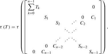
where

$$\begin{aligned} S_{j} =\sum _{k=0}^{n-1}\sin \left( \frac{2\pi jk}{n} \right) \, T_{k} \end{aligned}$$

and

$$\begin{aligned} C_{j} =\sum _{k=0}^{n-1}\cos \left( \frac{2\pi jk}{n} \right) \, T_{k} . \end{aligned}$$

• (2) If n is even, we have

  

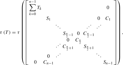
  where $S_j$ and $C_j$ are given above.

Proof

Let $U=\left[ U_{ij} \right] ,$ where $U_{ij} =\frac{1}{\sqrt{n} } \left[ \cos \left( \frac{2\pi (j-1)(i-1)}{n} \right) +\sin \left( \frac{2\pi (j-1)(i-1)}{n} \right) \right] \, \, I$, and I is the identity operator in $\mathscr {B}\left( H\right)$. Using the sums $\displaystyle \sum _{k=1}^{n}\sin \left( kx\right) =\frac{\sin \left( \frac{n+1}{2} x\right) \sin \left( \frac{nx}{2} \right) }{\mathrm{sin}\left( \frac{x}{2} \right) }$ and $\displaystyle \sum _{k=0}^{n}\cos \left( kx\right) =\frac{1}{2} \left( 1+\frac{\sin \left( \frac{2n+1}{2} x\right) }{\sin \left( \frac{x}{2} \right) } \right)$ (see, e.g., [10, p. 37]), one can prove that the set of column vectors of the $n\times n$ matrix given in the definition of U form an orthonormal set of vectors. Thus, U is a unitary operator in $\mathscr {B}\left( H^{\left( n\right) }\right)$ and, in view of the fact that $\displaystyle \sum _{k=0}^{n-1}\sin \left( \frac{2\pi jk}{n} \right) =\sum _{k=0}^{n-1}\cos \left( \frac{2\pi jk}{n} \right) =0$ for $j=1,\, 2,\, \ldots ,\, n-1$, we have

when n is odd, and

when n is even. $\square$

Hence, from the invariance property of weakly unitarily invariant norms, we have the desired result.

Based on Theorem 1, we have the following pinching inequalities.

Corollary 1

Let $T_0,\ T_1,\ \dots ,\ T_{n-1}\in \mathscr {B}\left( H\right)$ , T be an $n\times n$ Hankel operator matrix in $\mathscr {B}\left( H^{\left( n\right) }\right)$ given by . Then

• (1) If n is odd , we have

• (a) $\omega (T)\ge \max \left\{ \omega \left( \displaystyle \sum _{k=0}^{n-1}T_{k} \right) ,\, \omega \left( S_{j} \right) :j=1,2,\ldots ,n-1\right\}$, with equality when $C_{j} =0$ for all $j=1,\, 2,\, \ldots ,\, n-1.$

• (b) $\left\| T\right\| \ge \max \left\{ \left\| \displaystyle \sum _{k=0}^{n-1}T_{k} \right\| ,\, \, \left\| S_{j} \right\| :j=1,2,\ldots ,n-1\right\}$, with equality when $C_{j} =0$ for all $j=1,\, 2,\, \ldots ,\, n-1.$

• (c) $\left\| T\right\| _{p} \ge \left( \left\| \displaystyle \sum _{k=0}^{n-1}T_{k} \right\| _{p}^{p} +\displaystyle \sum _{j=1}^{n-1}\left\| S_{j} \right\| _{p}^{p} \right) ^{\frac{1}{p} }$ for $1\le p<\infty$. For $1< p<\infty$, equality holds if and only if $C_{j} =0$ for all $j=1,\, 2,\, \ldots ,\, n-1.$

• (2) If n is even, we have

• (a) $\omega (T)\ge \max \left\{ \omega \left( \displaystyle \sum _{k=0}^{n-1}T_{k} \right) ,\, \omega \left( S_{j} \right) ,\, \omega \left( C_{\frac{n}{2} } \right) :j=1,2,\ldots ,n-1,\, j\ne \frac{n}{2}\right\}$, with equality when $C_{j} =0$ for all $j=1,\, 2,\, \ldots ,\, n-1$, $j\ne \frac{n}{2}$.

• (b) $\left\| T\right\| \ge \max \left\{ \left\| \displaystyle \sum _{k=0}^{n-1}T_{k} \right\| ,\, \, \left\| S_{j} \right\| ,\, \left\| C_{\frac{n}{2} } \right\| :j=1,2,\ldots ,n-1,\, j\ne \frac{n}{2}\right\}$, with equality when $C_{j} =0$ for all $j=1,\, 2,\, \ldots ,\, n-1$, $j\ne \frac{n}{2}$.

• (c) $\left\| T\right\| _{p} \ge \left( \left\| \displaystyle \sum _{k=0}^{n-1}T_{k} \right\| _{p}^{p} +\displaystyle \sum _{\begin{array}{l} {j=1} \\ {j\ne \frac{n}{2}} \end{array}}^{n-1}\left\| S_{j} \right\| _{p}^{p} +\left\| C_{\frac{n}{2} } \right\| _{p}^{p} \right) ^{\frac{1}{p} }$ for $1\le p<\infty$. For $1< p<\infty$, equality holds if and only if $C_{j} =0$ for all $j=1,\, 2,\, \ldots ,\, n-1$, $j\ne \frac{n}{2}$.

Proof

Follows directly by Theorem 1 and the inequalities (1)–(4). $\square$

Corollary 2

Let $T_0,\ T_1,\ \dots ,\ T_{n-1}\in \mathscr {B}\left( H\right)$ , T be an $n\times n$ Hankel operator matrix in $\mathscr {B}\left( H^{\left( n\right) }\right)$ given by and let $\tau$ be any weakly unitarily invariant norm. Then

• (1) If n is odd , $T_{0} =\frac{T_{1} +T_{2} }{2}$, $T_{1} =T_{3} =T_{5} =\cdots =T_{n-2}$ and $T_{2} =T_{4} =T_{6} =\cdots =T_{n-1}$ , we have $\tau (T)=\tau \left( diag\left( \frac{n}{2} \left( T_{1} +T_{2} \right) ,\, D_{1} ,\, D_{2} ,\, \ldots ,\, D_{n-2} ,\, D_{n-1} \right) \right)$, where

  $$\begin{aligned} D_{j} =\sum _{\begin{array}{l} {k=0} \\ {k\, odd} \end{array}}^{n-1}\sin \left( \frac{2\pi jk}{n} \right) \, T_{1} +\sum _{\begin{array}{l} {k=0} \\ {k\, even} \end{array}}^{n-1}\sin \left( \frac{2\pi jk}{n} \right) \, T_{2}. \end{aligned}$$

• (2) If n is even, $T_{1} =T_{3} =T_{5} =\cdots =T_{n-1}\$and $T_{0} =T_{2} =T_{4} =\cdots =T_{n-2}$, we have

  $$\begin{aligned} \tau (T)&=\tau \left( diag\left( \frac{n}{2} \left( T_{0} +T_{1} \right) ,F_{1} ,F_{2} ,\ldots ,F_{\frac{n}{2} -1} ,\, \frac{n}{2} \left( T_{0} -T_{1} \right) ,\right. \right. \\&\quad \left. \left. F_{\frac{n}{2} +1} ,\ldots ,\, F_{n-2} ,\, F_{n-1} \right) \right) \\&=\tau \left( diag\left( \frac{n}{2} \left( T_{0} +T_{1} \right) ,\, \frac{n}{2} \left( T_{0} -T_{1} \right) \right) \right) ,\hbox { where}\\ F_{j}&=\sum _{\begin{array}{l} {k=0} \\ {k\, odd} \end{array}}^{n-1}\sin \left( \frac{2\pi jk}{n} \right) \, T_{1} +\sum _{\begin{array}{l} {k=0} \\ {k\, even} \end{array}}^{n-1}\sin \left( \frac{2\pi jk}{n} \right) \, T_{0}. \end{aligned}$$

Here we note that if n is even, then

$$\begin{aligned} \sum _{\begin{array}{l} {k=0} \\ {k\, odd} \end{array}}^{n-1}\sin \left( \frac{2\pi jk}{n} \right) \, =\ \sum _{\begin{array}{l} {k=0} \\ {k\, even} \end{array}}^{n-1}\sin \left( \frac{2\pi jk}{n} \right) \, =\ 0 \end{aligned}$$

for any $j\in \left\{ 1,\, 2,\, \ldots ,\, n-1\right\}$ (see, e.g., [10, p. 37]).

Proof

• (1) Follows by Theorem 1 and the identities

  $$\begin{aligned} \sum _{\begin{array}{l} {k=1} \\ {k\, odd} \end{array}}^{n-1}\cos \left( \frac{2\pi jk}{n} \right) \, =\frac{-1}{2} \end{aligned}$$

  and

  $$\begin{aligned} \sum _{\begin{array}{l} {k=1} \\ {k\, even} \end{array}}^{n-1}\cos \left( \frac{2\pi jk}{n} \right) \, =\frac{-1}{2}, \end{aligned}$$

  where $j=1,\, 2,\, \ldots ,\, n-1$ (see, e.g., [10, p. 37]).

• (2) Follows by Theorem 1 and the identities

  $$\begin{aligned} \sum _{\begin{array}{l} {k=0} \\ {k\, odd} \end{array}}^{n-1}\cos \left( \frac{2\pi jk}{n} \right) \, =\ 0 \end{aligned}$$

  and

  $$\begin{aligned} \sum _{\begin{array}{l} {k=0} \\ {k\, even} \end{array}}^{n-1}\cos \left( \frac{2\pi jk}{n} \right) \, =\ 0, \end{aligned}$$

  where $j=1,\, 2,\, \ldots ,\, n-1$, $j\ne \frac{n}{2}$ (see, e.g., [10, p. 37]).

Specializing the norm equality in part (i) of Corollary 2 to the numerical radius, the usual operator norm and to the Schatten p-norms, we obtain the following equalities:

• (a) $\omega (T)=\max \left\{ \frac{n}{2} \omega \left( T_{1} +T_{2} \right) ,\, \omega \left( D_{j} \right) :j=1,2,\ldots ,n-1\right\}$.

• (b) $\left\| T\right\| =\max \left\{ \frac{n}{2} \left\| T_{1} +T_{2} \right\| ,\, \left\| D_{j} \right\| :j=1,2,\ldots ,n-1\right\}$.

• (c) $\left\| T\right\| _{p} =\left( \left\| \frac{n\left( T_{1} +T_{2} \right) }{2} \right\| _{p}^{p} +\sum _{j=1}^{n-1}\left\| D_{j} \right\| _{p}^{p} \right) ^{\frac{1}{p} }$ for $1\le p<\infty$.

Specializing the norm equality in part (2) of Corollary 2 to the numerical radius, the usual operator norm and to the Schatten p-norms, we obtain the following equalities:

• (a) $\omega (T)=\frac{n}{2} \max \left\{ \omega \left( T_{0} +T_{1} \right) ,\, \, \omega \left( T_{0} -T_{1} \right) \right\}$.

• (b) $\left\| T\right\| =\frac{n}{2} \max \left\{ \left\| T_{0} +T_{1} \right\| ,\, \left\| T_{0} -T_{1} \right\| \right\} .$

• (c) $\left\| T\right\| _{p} =\frac{n}{2} \left( \left\| T_{0} +T_{1} \right\| _{p}^{p} +\left\| T_{0} -T_{1} \right\| _{p}^{p} \right) ^{\frac{1}{p} }$ for $1\le p<\infty$.

$\square$

Remark 1

Let $A,B\in \mathscr {B}\left( H\right)$ and let T be a $2\times 2$ Hankel operator matrix in $\mathscr {B}\left( H^{\left( 2\right) }\right)$ given by $T=\left[ \begin{array}{cc} A &{} B \\ B &{} A \end{array} \right]$. Then

$$\begin{aligned} \tau \left( T\right) =\tau \left( \left[ \begin{array}{cc} A-B &{} 0 \\ 0 &{} A+B \end{array} \right] \right) . \end{aligned}$$

To see this, let $U=\frac{1}{\sqrt{2}}\left[ \begin{array}{cc} 1 &{} 1 \\ 1 &{} -1 \end{array} \right] \otimes I$. Then it is easy to prove that U is a unitary operator in $\mathscr {B}\left( H^{\left( 2\right) }\right)$.

Now,

$$\begin{aligned} UTU^*=\left[ \begin{array}{cc} A+B &{} 0 \\ 0 &{} A-B \end{array} \right] . \end{aligned}$$

Hence, from the invariance property of weakly unitarily invariant norms, we have the desired result. This result can be found in [14].

Remark 2

Let $A,B,C\in \mathscr {B}\left( H\right)$ and let T be a $3\times 3$ Hankel operator matrix in $\mathscr {B}\left( H^{\left( 3\right) }\right)$ given by $T=\left[ \begin{array}{ccc} A &{} B &{} C \\ B &{} C &{} A \\ C &{} A &{} B \end{array} \right]$. Then

$$\begin{aligned} \tau \left( T\right) =\tau \left( \left[ \begin{array}{ccc} A+B+C &{} 0 &{} 0 \\ 0 &{} \frac{\sqrt{3}}{2}\left( B-C\right) &{} A-\frac{1}{2}\left( B+C\right) \\ 0 &{} A-\frac{1}{2}\left( B+C\right) &{} \frac{\sqrt{3}}{2}\left( C-B\right) \end{array} \right] \right) . \end{aligned}$$

To see this, let $U=\frac{1}{\sqrt{3}}\left[ \begin{array}{ccc} 1 &{} 1 &{} 1 \\ 1 &{} -\frac{1}{2}+\frac{\sqrt{3}}{2} &{} -\frac{1}{2}-\frac{\sqrt{3}}{2} \\ 1 &{} -\frac{1}{2}-\frac{\sqrt{3}}{2} &{} -\frac{1}{2}+\frac{\sqrt{3}}{2} \end{array} \right] \otimes I$. Then it is easy to prove that U is a unitary operator in $\mathscr {B}\left( H^{\left( 3\right) }\right)$.

Now,

$$\begin{aligned} UTU^*=\left[ \begin{array}{ccc} A+B+C &{} 0 &{} 0 \\ 0 &{} \frac{\sqrt{3}}{2}\left( B-C\right) &{} A-\frac{1}{2}\left( B+C\right) \\ 0 &{} A-\frac{1}{2}\left( B+C\right) &{} \frac{\sqrt{3}}{2}\left( C-B\right) \end{array} \right] . \end{aligned}$$

Hence, from the invariance property of weakly unitarily invariant norms we have the desired result.

Note that if $A=\frac{B+C}{2}$ in Remark 2, then we get the following result:

$$\begin{aligned} \tau \left( T\right) =\tau \left( diag\left( \frac{3}{2}(B+C),\ \frac{\sqrt{3}}{2}\left( B-C\right) ,\frac{\sqrt{3}}{2}\left( C-B\right) \ \right) \right) . \end{aligned}$$

Now, specializing the norm equality in the last equality to the numerical radius, the usual operator norm, and to the Schatten p-norms, we obtain the following equalities:

• 1. $\omega \left( \left[ \begin{array}{ccc} \frac{B+C}{2} &{} B &{} C \\ B &{} C &{} \frac{B+C}{2} \\ C &{} \frac{B+C}{2} &{} B \end{array} \right] \right) =max\left\{ \frac{3}{2}\omega \left( (B+C)\right) ,\ \frac{\sqrt{3}}{2}\omega \left( \left( B-C\right) \right) \right\}$.

• 2. $\left\| \left[ \begin{array}{ccc} \frac{B+C}{2} &{} B &{} C \\ B &{} C &{} \frac{B+C}{2} \\ C &{} \frac{B+C}{2} &{} B \end{array} \right] \right\| =max\left\{ \frac{3}{2}\left\| B+C\right\| ,\ \frac{\sqrt{3}}{2}\left\| B-C\right\| \right\} .$

• 3. ${\left\| \left[ \begin{array}{ccc} \frac{B+C}{2} &{} B &{} C \\ B &{} C &{} \frac{B+C}{2} \\ C &{} \frac{B+C}{2} &{} B \end{array} \right] \right\| }^p_p={\left\| \frac{3}{2}(B+C)\right\| }^p_p+2{\left\| \frac{\sqrt{3}}{2}\left( B-C\right) \right\| }^p_p$

for $1\le p<\infty$.

Remark 3

Let $A,B,C,D\in \mathscr {B}\left( H\right)$ and let T be a $4\times 4$ Hankel operator matrix in $\mathscr {B}\left( H^{\left( 4\right) }\right)$ given by $T=\left[ \begin{array}{cccc} A &{} B &{} C &{} D\\ B &{} C &{} D &{} A\\ C &{} D &{} A &{} B\\ D &{} A &{} B &{} C\\ \end{array} \right]$. Then

$\tau \left( T\right) =\tau \left( \left[ \begin{array}{cccc} M_1 &{} 0 &{} 0 &{} 0\\ 0 &{} M_2 &{} 0 &{} N\\ 0 &{} 0 &{} M_3 &{} 0\\ 0 &{} N &{} 0 &{} M_4\\ \end{array} \right] \right)$, where

$M_1=A+B+C+D$, $M_2=B-D$, $M_3=A-B+C-D$, $M_4=D-B$, and $N=A-C$.

To see this, let $U=\frac{1}{2} \left[ \begin{array}{cccc} {1} &{} {1} &{} {1} &{} {1} \\ {1} &{} {1} &{} {-1} &{} {-1} \\ {1} &{} {-1} &{} {1} &{} {-1} \\ {1} &{} {-1} &{} {-1} &{} {1} \end{array}\right] \otimes I.$ Then it is easy to prove that U is a unitary operator in $\mathscr {B}\left( H^{\left( 4\right) }\right)$.

Now,

$UTU^*=\left[ \begin{array}{cccc} M_1 &{} 0 &{} 0 &{} 0\\ 0 &{} M_2 &{} 0 &{} N\\ 0 &{} 0 &{} M_3 &{} 0\\ 0 &{} N &{} 0 &{} M_4\\ \end{array} \right] ,$ where $M_{1} ,\, M_{2} ,\, M_{3} ,\, M_{4} ,\, N \$are given above.

Hence, from the invariance property of weakly unitarily invariant norms we have the desired result.

Note that If $A=C$ in Remark 3, then we get the following result:

$$\begin{aligned} \tau \left( T\right) =\tau \left( diag\left( 2A+B+D,B-D,2A-B-D,\ D-B\right) \right) . \end{aligned}$$

Now, specializing the norm equality in the last equality to the numerical radius, the usual operator norm, and to the Schatten p-norms, we obtain the following equalities:

• 1. $\omega \left( \left[ \begin{array}{cccc} A &{} B &{} A &{} D \\ B &{} A &{} D &{} A \\ A &{} D &{} A &{} B \\ D &{} A &{} B &{} A \\ \end{array} \right] \right) =max\left\{ \omega \left( 2A+B+D\right) ,\ \omega \left( B-D\right) ,\ \omega \left( 2A-B-D\right) \right\}$.

• 2. $\left\| \left[ \begin{array}{cccc} A &{} B &{} A &{} D \\ B &{} A &{} D &{} A \\ A &{} D &{} A &{} B \\ D &{} A &{} B &{} A \\ \end{array} \right] \right\| =max\left\{ \left\| 2A+B+D\right\| ,\left\| B-D\right\| ,\left\| 2A-B-D\right\| \right\} .$

• 3. ${\left\| \left[ \begin{array}{cccc} A &{} B &{} A &{} D \\ B &{} A &{} D &{} A \\ A &{} D &{} A &{} B \\ D &{} A &{} B &{} A \\ \end{array} \right] \right\| }^p_p={\left\| 2A+B+D\right\| }^p_p+2{\left\| B-D\right\| }^p_p+{\left\| 2A-B-D\right\| }^p_p$ for $1\le p<\infty$.

Remark 4

Let $A,\ B,\ C,\ D\in \mathscr {B}\left( H\right)$ and let T be a $4\times 4$ Hankel operator matrix in $\mathscr {B}\left( H^{\left( 4\right) }\right)$ given by $T=\left[ \begin{array}{cccc} {A} &{} {B} &{} {C} &{} {D} \\ {B} &{} {A} &{} {D} &{} {C} \\ {C} &{} {D} &{} {A} &{} {B} \\ {D} &{} {C} &{} {B} &{} {A} \end{array}\right]$. Then

$$\begin{aligned} \tau \left( T\right) =\tau \left( \left[ \begin{array}{cccc} {A+B+C+D} &{} {0} &{} {0} &{} {0} \\ {0} &{} {A+B-C-D} &{} {0} &{} {0} \\ {0} &{} {0} &{} {A-B+C-D} &{} {0} \\ {0} &{} {0} &{} {0} &{} {A-B-C+D} \end{array}\right] \right) . \end{aligned}$$

To see this, let $U=\frac{1}{2} \left[ \begin{array}{cccc} {1} &{} {1} &{} {1} &{} {1} \\ {1} &{} {1} &{} {-1} &{} {-1} \\ {1} &{} {-1} &{} {1} &{} {-1} \\ {1} &{} {-1} &{} {-1} &{} {1} \end{array}\right] \otimes I.$ Then it is easy to prove that U is a unitary operator in $\mathscr {B}\left( H^{\left( 4\right) }\right)$.

Now,

$$\begin{aligned} UTU^{*} =diag\left( A+B+C+D,\, A+B-C-D, A-B+C-D,\, A-B-C+D\right) . \end{aligned}$$

Hence, from the invariance property of weakly unitarily invariant norms we have the desired result.

Now, specializing the norm equality in Remark 4 to the numerical radius, the usual operator norm, and to the Schatten p-norms, we obtain the following equalities:

• 1. $\omega \left( \left[ \begin{array}{cccc} A &{} B &{} C &{} D \\ B &{} A &{} D &{} C \\ C &{} D &{} A &{} B \\ D &{} C &{} B &{} A \\ \end{array} \right] \right) = max\left\{ \omega \left( A+B+C+D\right) ,\ \omega \left( A+B-C-D\right) ,\right. \left. \omega \left( A-B+C-D\right) ,\ \omega \left( A-B-C+D\right) \right\}$.

• 2. $\left\| \left[ \begin{array}{cccc} A &{} B &{} C &{} D \\ B &{} A &{} D &{} C \\ C &{} D &{} A &{} B \\ D &{} C &{} B &{} A \\ \end{array} \right] \right\| =max\left\{ \left\| A+B+C+D\right\| ,\ \left\| A+B-C-D\right\| ,\left\| A-B\right. \right. \left. \left. +C-D\right\| ,\ \left\| A-B-C+D\right\| \right\}$.

• 3. ${\left\| \left[ \begin{array}{cccc} A &{} B &{} C &{} D \\ B &{} A &{} D &{} C \\ C &{} D &{} A &{} B \\ D &{} C &{} B &{} A \\ \end{array} \right] \right\| }^p_p ={\left\| A+B+C+D\right\| }^p_p+{\left\| A+B-C-D\right\| }^p_p+{\Big \Vert A-B+C-D\Big \Vert }^p_p +{\left\| A-B-C+D\right\| }^p_p \hbox {for} 1\le p<\infty$.

Special cases of Remark 4:

• (1) If $A=B=C=D$, then $UTU^{*} =diag\left( 4A,\, 0,\, 0,\, 0\right)$.

• (2) If $B=C=0$, then $UTU^{*} =diag\left( A+D,\, A-D,\, A-D,\, A+D\right)$.

• (3) If $B=-C$ and $D=0$, then $UTU^{*} =diag\left( A,\, A+2B,\, A-2B,\, A\right)$.

• (4) If $A=D=0$, then $UTU^{*} =diag\left( B+C,\, B-C,\, C-B,\, -(B+C)\right)$.

• (5) If $C=iB$ and $D=0$, then $UTU^{*} =diag\left( A+(1+i)B,\, A+(1-i)B,\, A+(-1+i)B,\, A-(1+i)B\right)$.

• (6) If $A=C$, then $UTU^{*} =diag\left( 2A+B+D,\, B-D,\, 2A-B-D,\, D-B\right)$.

Remark 5

Let $A,B,C,D,E\in \mathscr {B}\left( H\right)$ and let T be a $5\times 5$ Hankel operator matrix in $\mathscr {B}\left( H^{\left( 5\right) }\right)$ given by $T=\left[ \begin{array}{ccccc} A &{} B &{} C &{} D &{} E\\ B &{} C &{} D &{} E &{} A\\ C &{} D &{} E &{} A &{} B\\ D &{} E &{} A &{} B &{} C\\ E &{} A &{} B &{} C &{} D\\ \end{array} \right]$. Then

$\tau \left( T\right) =\tau \left( \left[ \begin{array}{ccccc} W_1 &{} 0 &{} 0 &{} 0 &{} 0 \\ 0 &{} W_2 &{} 0 &{} 0 &{} V_1 \\ 0 &{} 0 &{} W_3 &{} V_2 &{} 0\\ 0 &{} 0 &{} V_2 &{} W_4 &{} 0\\ 0 &{} V_1 &{} 0 &{} 0 &{} W_5\\ \end{array}\right] \right)$, where

$W_1=A+B+C+D+E$, $W_2=sin\frac{4\pi }{5}\left( C-D\right) +sin\frac{2\pi }{5}\left( B-E\right)$, $W_3=sin\frac{2\pi }{5}\left( D-C\right) +{\mathrm {sin} \frac{4\pi }{5}\left( B-E\right) \ }$, $W_4=sin\frac{2\pi }{5}\left( C-D\right) +{\mathrm {sin} \frac{4\pi }{5}\left( E-B\right) \ }$, $W_5=sin\frac{2\pi }{5}\left( E-B\right) +{\mathrm {sin} \frac{4\pi }{5}\left( D-C\right) \ }$, $V_1=A+cos\frac{2\pi }{5}\left( B+E\right) +cos\frac{4\pi }{5}\left( C+D\right)$ and $V_2=A+cos\frac{4\pi }{5}\left( B+E\right) +cos\frac{2\pi }{5}\left( C+D\right)$.

To see this, let $U=\frac{1}{\sqrt{5} } \left[ \begin{array}{ccccc} {1} &{} {1} &{} {1} &{} {1} &{} {1} \\ {1} &{} {\alpha _{1} } &{} {\alpha _{2} } &{} {\alpha _{3} } &{} {\alpha _{4} } \\ {1} &{} {\alpha _{2} } &{} {\alpha _{4} } &{} {\alpha _{1} } &{} {\alpha _{3} } \\ {1} &{} {\alpha _{3} } &{} {\alpha _{1} } &{} {\alpha _{4} } &{} {\alpha _{2} } \\ {1} &{} {\alpha _{4} } &{} {\alpha _{3} } &{} {\alpha _{2} } &{} {\alpha _{1} } \end{array}\right] \otimes I$, where

$\alpha _{j} =\cos \left( \frac{2\pi j}{5} \right) +\sin \left( \frac{2\pi j}{5} \right)$. Then it is easy to prove that U is a unitary operator in $\mathscr {B}\left( H^{\left( 5\right) }\right)$.

Now,

$UTU^*=\left[ \begin{array}{ccccc} W_1 &{} 0 &{} 0 &{} 0 &{} 0 \\ 0 &{} W_2 &{} 0 &{} 0 &{} V_1 \\ 0 &{} 0 &{} W_3 &{} V_2 &{} 0\\ 0 &{} 0 &{} V_2 &{} W_4 &{} 0\\ 0 &{} V_1 &{} 0 &{} 0 &{} W_5\\ \end{array} \right] ,$ where $W_i\ and\ V_j\$are given above.

Hence, from the invariance property of weakly unitarily invariant norms we have the desired result.

Note that if $A=\frac{B+C}{2}\ ,\ B=D\ ,\ and\ C=E$ in Remark 5, then we get the following result:

$$\begin{aligned} \tau \left( T\right) =\tau \left( \begin{array}{c} diag\left( \begin{array}{c} \frac{5}{2}\left( B+C\right) ,\ \ \left( sin\frac{4\pi }{5}-sin\frac{2\pi }{5}\right) \left( C-B\right) ,\ \ \left( sin\frac{2\pi }{5}+sin\frac{4\pi }{5}\right) \left( B-C\right) ,\ \ \ \\ \left( sin\frac{2\pi }{5}+sin\frac{4\pi }{5}\right) \left( C-B\right) ,\ \ \ \left( sin\frac{2\pi }{5}-sin\frac{4\pi }{5}\right) \left( C-B\right) \end{array} \right) \\ \ \ \end{array} \right) . \end{aligned}$$

Now, specializing the norm equality in the last equality to the numerical radius, the usual operator norm, and to the Schatten p-norms, we obtain the following equalities:

• 1. $\omega \left( \left[ \begin{array}{ccccc} {\frac{B+C}{2} } &{} {B} &{} {C} &{} {B} &{} {C} \\ {B} &{} {C} &{} {B} &{} {C} &{} {\frac{B+C}{2} } \\ {C} &{} {B} &{} {C} &{} {\frac{B+C}{2} } &{} {B} \\ {B} &{} {C} &{} {\frac{B+C}{2} } &{} {B} &{} {C} \\ {C} &{} {\frac{B+C}{2} } &{} {B} &{} {C} &{} {B} \end{array}\right] \right) = max\left\{ \begin{array}{c} \omega \left( \frac{5}{2}\left( B+C\right) \right) ,\ \omega \left( \left( sin\frac{4\pi }{5}-sin\frac{2\pi }{5}\right) \left( C-B\right) \right) ,\ \\ \omega \left( \left( sin\frac{2\pi }{5}+sin\frac{4\pi }{5}\right) \left( B-C\right) \right) \end{array} \right\}$.

• 2. $\left\| \left[ \begin{array}{ccccc} {\frac{B+C}{2} } &{} {B} &{} {C} &{} {B} &{} {C} \\ {B} &{} {C} &{} {B} &{} {C} &{} {\frac{B+C}{2} } \\ {C} &{} {B} &{} {C} &{} {\frac{B+C}{2} } &{} {B} \\ {B} &{} {C} &{} {\frac{B+C}{2} } &{} {B} &{} {C} \\ {C} &{} {\frac{B+C}{2} } &{} {B} &{} {C} &{} {B} \end{array}\right] \right\| =max\left\{ \begin{array}{c} \left\| \frac{5}{2}\left( B+C\right) \right\| ,\left\| \left( sin\frac{4\pi }{5}-sin\frac{2\pi }{5}\right) \left( C-B\right) \right\| , \\ \left\| \left( sin\frac{2\pi }{5}+sin\frac{4\pi }{5}\right) \left( B-C\right) \right\| \ \end{array} \right\}$.

• 3. ${\left\| \left[ \begin{array}{ccccc} {\frac{B+C}{2} } &{} {B} &{} {C} &{} {B} &{} {C} \\ {B} &{} {C} &{} {B} &{} {C} &{} {\frac{B+C}{2} } \\ {C} &{} {B} &{} {C} &{} {\frac{B+C}{2} } &{} {B} \\ {B} &{} {C} &{} {\frac{B+C}{2} } &{} {B} &{} {C} \\ {C} &{} {\frac{B+C}{2} } &{} {B} &{} {C} &{} {B} \end{array}\right] \right\| }^p_p ={\left\| \frac{5}{2}\left( B+C\right) \right\| }^p_p+\ {2\left\| \left( sin\frac{4\pi }{5}-sin\frac{2\pi }{5}\right) \left( C-B\right) \right\| }^p_p + {2\left\| \left( sin\frac{2\pi }{5}+sin\frac{4\pi }{5}\right) \left( B-C\right) \right\| }^p_p\ \hbox { for } 1\le p<\infty$.

Remark 6

Let $A,B,C,D,E,F\in \mathscr {B}\left( H\right)$ and let T be a $6\times 6$ Hankel operator matrix in $\mathscr {B}\left( H^{\left( 6\right) }\right)$ given by $T=\left[ \begin{array}{cccccc} A &{} B &{} C &{} D &{} E &{} F\\ B &{} C &{} D &{} E &{} F &{} A\\ C &{} D &{} E &{} F &{} A &{} B \\ D &{} E &{} F &{} A &{} B &{} C\\ E &{} F &{} A &{} B &{} C &{} D\\ F &{} A &{} B &{} C &{} D &{} E \end{array}\right]$. Then

$\tau \left( T\right) =\tau \left( \left[ \begin{array}{cccccc} K_1 &{} 0 &{} 0 &{} 0 &{} 0 &{} 0 \\ 0 &{} K_2 &{} 0 &{} 0 &{} 0 &{} L_1 \\ 0 &{} 0 &{} K_3 &{} 0 &{} L_2 &{} 0\\ 0 &{} 0 &{} 0 &{} K_4 &{} 0 &{} 0\\ 0 &{} 0 &{} L_2 &{} 0 &{} K_5 &{} 0 \\ 0 &{} L_1 &{} 0 &{} 0 &{} 0 &{} K_6 \end{array} \right] \right)$ , where

$$\begin{aligned} K_1= & {} A+B+C+D+E+F, K_2=\frac{\sqrt{3}}{2}\left( B+C-E-F\right) , K_3\\= & {} \frac{\sqrt{3}}{2}\left( B-C+E-F\right) \\ K_4= & {} A-B+C-D+E-F, K_5=\frac{\sqrt{3}}{2}\left( -B+C-E+F\right) , K_6\\= & {} \frac{\sqrt{3}}{2}\left( -B-C+E+F\right) \\ L_1= & {} \left( A-D\right) +\frac{1}{2}\left( B-C-E+F\right) , \hbox {and}\, L_2=\left( A+D\right) +\frac{1}{2}\left( -B-C-E-F\right) . \end{aligned}$$

To see this, let $U=\frac{1}{\sqrt{6}}\left[ \begin{array}{cccccc} 1 &{} 1 &{} 1 &{} 1 &{} 1 &{} 1\\ 1 &{} \mu &{} \rho &{} -1 &{} -\mu &{} -\rho \\ 1 &{} \rho &{} -\mu &{} 1 &{} \rho &{} -\mu \\ 1 &{} -1 &{} 1 &{} -1 &{} 1 &{} -1\\ 1 &{} -\mu &{} \rho &{} 1 &{} -\mu &{} \rho \\ 1 &{} -\rho &{} -\mu &{} -1 &{} \rho &{} \mu \\ \end{array} \right] \otimes I$, where

$\mu =\frac{1}{2}+\frac{\sqrt{3}}{2}$ , $\rho =-\frac{1}{2}+\frac{\sqrt{3}}{2}$. Then it is easy to prove that U is a unitary operator in $\mathscr {B}\left( H^{\left( 6\right) }\right)$ and

$$\begin{aligned} UTU^*=\left[ \begin{array}{cccccc} K_1 &{} 0 &{} 0 &{} 0 &{} 0 &{} 0 \\ 0 &{} K_2 &{} 0 &{} 0 &{} 0 &{} L_1 \\ 0 &{} 0 &{} K_3 &{} 0 &{} L_2 &{} 0\\ 0 &{} 0 &{} 0 &{} K_4 &{} 0 &{} 0\\ 0 &{} 0 &{} L_2 &{} 0 &{} K_5 &{} 0 \\ 0 &{} L_1 &{} 0 &{} 0 &{} 0 &{} K_6 \end{array} \right] . \end{aligned}$$

Hence, from the invariance property of weakly unitarily invariant norms we have the desired result.

Note that if $A=\frac{C+E}{2}$ and $D=\frac{B+F}{2}$ in Remark 6, then we get the following result

$$\begin{aligned}&\tau \left( \left[ \begin{array}{cccccc} \frac{C+E}{2} &{} B &{} C &{} \frac{B+F}{2} &{} E &{} F \\ B &{} C &{} \frac{B+F}{2} &{} E &{} F &{} \frac{C+E}{2} \\ C &{} \frac{B+F}{2} &{} E &{} F &{} \frac{C+E}{2} &{} B \\ \frac{B+F}{2} &{} E &{} F &{} \frac{C+E}{2} &{} B &{} C \\ E &{} F &{} \frac{C+E}{2} &{} B &{} C &{} \frac{B+F}{2} \\ F &{} \frac{C+E}{2} &{} B &{} C &{} \frac{B+F}{2} &{} E \\ \end{array} \right] \right) \\&\quad =\tau \left( \left[ \begin{array}{cccccc} X_1 &{} 0 &{} 0 &{} 0 &{} 0 &{} 0\\ 0 &{} X_2 &{} 0 &{} 0 &{} 0 &{} 0\\ 0 &{} 0 &{} X_3 &{} 0 &{} 0 &{} 0\\ 0 &{} 0 &{} 0 &{} X_4 &{} 0 &{} 0\\ 0 &{} 0 &{} 0 &{} 0 &{} X_5 &{} 0\\ 0 &{} 0 &{} 0 &{} 0 &{} 0 &{} X_6\\ \end{array} \right] \right) , \hbox { where}\\&X_1=\frac{3}{2}\left( B+C+E+F\right) , X_2=\frac{\sqrt{3}}{2}\left( B+C-E-F\right) ,\\&X_3=\frac{\sqrt{3}}{2}\left( B-C+E-F\right) , \\&X_4=\frac{3}{2}\left( -B+C+E-F\right) , \ X_5=\frac{\sqrt{3}}{2}\left( -B+C-E+F\right) , \hbox {and} \\&X_6=\frac{\sqrt{3}}{2}\left( -B-C+E+F\right) . \end{aligned}$$

Specializing the norm equality in the last equality to the numerical radius, the usual operator norm, and to the Schatten p-norms, we obtain the following equalities:

• 1.
  $$\begin{aligned}&\omega \left( \left[ \begin{array}{cccccc} \frac{C+E}{2} &{} B &{} C &{} \frac{B+F}{2} &{} E &{} F \\ B &{} C &{} \frac{B+F}{2} &{} E &{} F &{} \frac{C+E}{2} \\ C &{} \frac{B+F}{2} &{} E &{} F &{} \frac{C+E}{2} &{} B \\ \frac{B+F}{2} &{} E &{} F &{} \frac{C+E}{2} &{} B &{} C \\ E &{} F &{} \frac{C+E}{2} &{} B &{} C &{} \frac{B+F}{2} \\ F &{} \frac{C+E}{2} &{} B &{} C &{} \frac{B+F}{2} &{} E \\ \end{array} \right] \right) =max\left\{ \omega \left( X_i\right) :i=1,\ 2,\ 3,\ 4\right\} . \end{aligned}$$
• 2.
  $$\begin{aligned} \left\| \left[ \begin{array}{cccccc} \frac{C+E}{2} &{} B &{} C &{} \frac{B+F}{2} &{} E &{} F \\ B &{} C &{} \frac{B+F}{2} &{} E &{} F &{} \frac{C+E}{2} \\ C &{} \frac{B+F}{2} &{} E &{} F &{} \frac{C+E}{2} &{} B \\ \frac{B+F}{2} &{} E &{} F &{} \frac{C+E}{2} &{} B &{} C \\ E &{} F &{} \frac{C+E}{2} &{} B &{} C &{} \frac{B+F}{2} \\ F &{} \frac{C+E}{2} &{} B &{} C &{} \frac{B+F}{2} &{} E \\ \end{array} \right] \right\| =max\left\{ \left\| X_i\right\| :i=1,\ 2,\ 3,\ 4\right\} . \end{aligned}$$
• 3.
  $$\begin{aligned} {\left\| \left[ \begin{array}{cccccc} \frac{C+E}{2} &{} B &{} C &{} \frac{B+F}{2} &{} E &{} F \\ B &{} C &{} \frac{B+F}{2} &{} E &{} F &{} \frac{C+E}{2} \\ C &{} \frac{B+F}{2} &{} E &{} F &{} \frac{C+E}{2} &{} B \\ \frac{B+F}{2} &{} E &{} F &{} \frac{C+E}{2} &{} B &{} C \\ E &{} F &{} \frac{C+E}{2} &{} B &{} C &{} \frac{B+F}{2} \\ F &{} \frac{C+E}{2} &{} B &{} C &{} \frac{B+F}{2} &{} E \\ \end{array} \right] \right\| }_p= \left( \displaystyle \sum _{i=1}^{6}\left\| X_{i} \right\| _{p}^{p} \right) ^{\frac{1}{p} } \hbox { for } 1\le p<\infty . \end{aligned}$$

3 New Inequalities

The results in this section are inequalities for $n\times n$ Hankel operator matrices. The following four lemmas can be found in [11, p. 48], [12], and [13, p. 44], respectively.

Lemma 1

Let $A\in \mathscr {B}\left( H\right)$. Then $r\left( A^{k} \right) =\left( r\left( A\right) \right) ^{k}$ for $k=1,\, 2,\, \ldots$ .

Lemma 2

Let $A\in \mathscr {B}\left( H\right)$. Then $\omega \left( \left[ \begin{array}{cc} {0} &{} {A} \\ {A} &{} {0} \end{array}\right] \right) =\omega \left( A\right)$.

Lemma 3

Let $H_{1} ,\, H_{2} ,\, \ldots ,\, H_{n}$ be Hilbert spaces, and let $T=\left[ T_{ij} \right]$ be $n\times n$ operator matrix with $T_{ij} \in \mathscr {B}\left( H_{j} ,\, H_{i} \right)$. Then $\omega \left( T\right) \le \omega \left( \left[ t_{ij}^{\wedge } \right] \right)$,

where

$$\begin{aligned} t_{ij}^{\wedge } =\left\{ \begin{array}{l} {\omega \left( T_{ij} \right) \, \, \, \, \, \, \, \, \, \, \, \, \, \, \, \, \, \, \, \, \, \, \, \, \, \, \, \, \, \, \, \, \, \, \, \, \, \, \, \, \, \, \, \, \mathrm{if}\, i=j,} \\ {\omega \left( \left[ \begin{array}{cc} {0} &{} {T_{ij} } \\ {T_{ji} } &{} {0} \end{array}\right] \right) \, \, \, \, \, \, \, \, \mathrm{if}\, i\ne j.} \end{array}\right. \, \, \, \, \, \, \, \, \, \, \, \, \, \, \, \, \end{aligned}$$

Lemma 4

If $A=\left[ a_{ij} \right] \in M_{n} \left( \mathrm{C}\right)$ with $a_{ij} \ge 0$, where $M_{n} \left( \mathrm{C}\right)$ is the algebra of all $n\times n$ complex matrices. Then $\omega \left( A\right) =r\left( Re\left( A\right) \right)$, where $Re\left( A\right) =\frac{1}{2} \left( A+A^{*} \right)$ is the real part of A.

Theorem 2

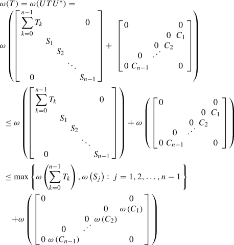
Let $T_0,\ T_1,\ \dots ,\ T_{n-1}\in \mathscr {B}\left( H\right)$ and . Then

• (1) Case1 If n is odd, we have

  $$\begin{aligned} \omega \left( T\right)\le & {} \max \left\{ \omega \left( \sum _{k=0}^{n-1}T_{k} \right) ,\omega \left( S_{j} \right) :\, j=1,2,\ldots ,n-1\, \right\} \\&+\max \left\{ \omega \left( C_{j} \right) :\, j=1,2,\ldots ,n-1\, \right\} , \end{aligned}$$

  with equality if $T_{0} =\frac{T_{1} +T_{2} }{2}$, $T_{1} =T_{3} =T_{5} =\cdots =T_{n-2}$ and $T_{2} =T_{4} =T_{6} =\cdots =T_{n-1}$.

Case 2 If n is even, we have

$$\begin{aligned} \begin{array}{l} {\omega \left( T\right) \le \max \left\{ \omega \left( \displaystyle \sum _{k=0}^{n-1}T_{k} \right) ,\omega \left( S_{j} \right) ,\, \omega \left( C_{\frac{n}{2} } \right) :\, j=1,2,\ldots ,n-1 , \, j\ne \frac{n}{2} \right\} } \\ \qquad \qquad \quad \,\,+{ \max \left\{ \omega \left( C_{j} \right) :\, j=1,2,\ldots ,n-1\, \, \mathrm{and}\, \, j\ne \frac{n}{2} \, \right\} ,} \end{array} \end{aligned}$$

with equality if $T_{1} =T_{3} =T_{5} =\cdots =T_{n-1}\$and $T_{0} =T_{2} =T_{4} =\cdots =T_{n-2}$.

• (2) Case 1 If n is odd, we have

  $$\begin{aligned} \left\| T\right\|&\le \max \left\{ \left\| \sum _{k=0}^{n-1}T_{k} \right\| ,\left\| \, S_{j} \right\| :\, j=1,2,\ldots ,n-1\, \right\} \\&\quad +\max \left\{ \left\| \, C_{j} \right\| :\, j=1,2,\ldots ,n-1\, \right\} , \end{aligned}$$

  with equality if $T_{0} =\frac{T_{1} +T_{2} }{2}$, $T_{1} =T_{3} =T_{5} =\cdots =T_{n-2}$ and $T_{2} =T_{4} =T_{6} =\cdots =T_{n-1}$. Case 2 If n is even, we have

  $$\begin{aligned} \left\| T\right\|&\le \max \left\{ \left\| \sum _{k=0}^{n-1}T_{k} \right\| ,\left\| \, S_{j} \right\| ,\, \left\| \, C_{\frac{n}{2} } \right\| :\, j=1,2,\ldots ,n-1 , \, j\ne \frac{n}{2} \right\} \\&\quad + \max \left\{ \left\| \, C_{j} \right\| :\, j=1,2,\ldots ,n-1\, \, \mathrm{and}\, j\ne \frac{n}{2} \, \right\} , \ \ \ \ \ \ \ \ \ \ \ \ \ \ \ \ \ \ \ \ \ \ \end{aligned}$$

  with equality if $T_{1} =T_{3} =T_{5} =\cdots =T_{n-1}\$and $T_{0} =T_{2} =T_{4} =\cdots =T_{n-2}$.

• (3) Case1 If n is odd, we have

  $$\begin{aligned} \left\| T\right\| _p \le \left( \left\| \displaystyle \sum _{k=0}^{n-1}T_{k} \right\| ^p_p +\displaystyle \sum _{j=1}^{n-1}\left\| S_{j} \right\| ^p_p \right) ^{\frac{1}{p} }+\left( \displaystyle \sum _{j=1}^{n-1}\left\| C_{j} \right\| ^p_p\right) ^{\frac{1}{p} } \end{aligned}$$

  with equality if $T_{0} =\frac{T_{1} +T_{2} }{2}$, $T_{1} =T_{3} =T_{5} =\cdots =T_{n-2}$ and $T_{2} =T_{4} =T_{6} =\cdots =T_{n-1}$.

  Case 2 If n is even, we have

  $$\begin{aligned} \left\| T\right\| _p \le \left( \left\| \displaystyle \sum _{k=0}^{n-1}T_{k} \right\| ^p_p +\displaystyle \sum _{\begin{array}{l} {j=1} \\ {j\ne \frac{n}{2}} \end{array}}^{n-1}\left\| S_{j} \right\| _{p}^{p} +\left\| C_{\frac{n}{2}}\right\| ^p_p \right) ^{\frac{1}{p}} +\left( \displaystyle \sum _{\begin{array}{l}{j=1} \\ {j\ne \frac{n}{2}} \end{array}}^{n-1}\left\| C_{j} \right\| ^p_p\right) ^{\frac{1}{p}} \end{aligned}$$

  with equality if $T_{1} =T_{3} =T_{5} =\cdots =T_{n-1}\$and $T_{0} =T_{2} =T_{4} =\cdots =T_{n-2}$.

Proof

• (1) Case1 Using U in Theorem 1, we get

  

(by Lemma 3, the identity $C_{j} =C_{n-j}$, and Lemma 2)

(by Lemma 4 and the identity $C_{j} =C_{n-j}$)

$$\begin{aligned}&=\max \left\{ \omega \left( \sum _{k=0}^{n-1}T_{k} \right) ,\omega \left( S_{j} \right) :\, j=1,2,\ldots ,n-1\, \right\} \\&\quad +\left( r\left( \, \left[ \begin{array}{ccccc} {0} &{} {} &{} {} &{} {} &{} {0} \\ {} &{} {\omega ^{2} \left( C_{1} \right) } &{} {} &{} {} &{} {} \\ {} &{} {} &{} {\omega ^{2} \left( C_{2} \right) } &{} {} &{} {} \\ {} &{} {} &{} {} &{} {\ddots } &{} {} \\ {0} &{} {} &{} {} &{} {} &{} {\omega ^{2} \left( C_{n-1} \right) } \end{array}\right] \, \right) \right) ^{\frac{1}{2} } \end{aligned}$$

(by Lemma 1 when $k=2$)

$$\begin{aligned}&=\max \left\{ \omega \left( \sum _{k=0}^{n-1}T_{k} \right) ,\omega \left( S_{j} \right) :\, j=1,2,\ldots ,n-1\, \right\} \\&\quad +\max \left\{ \omega \left( C_{j} \right) :\, j=1,2,\ldots ,n-1\, \right\} . \end{aligned}$$

The equality conditions follow from Corollary 2. $\square$

Case 2 Using U in Theorem 1, we get

( by Lemma 3 and the identity $C_{j} = C_{n-j}$ )

(by Lemma 4 and the identity $C_{j} =C_{n-j}$ )

$$\begin{aligned}&=\max \left\{ \omega \left( \sum _{k=0}^{n-1}T_{k} \right) ,\omega \left( S_{j} \right) ,\, \omega \left( C_{\frac{n}{2} } \right) :\, j=1,2,\ldots ,n-1 , \, j\ne \frac{n}{2} \right\} \\&\quad + \left( r\left( \left[ \begin{array}{cccccccc} {0} &{} {} &{} {} &{} {} &{} {} &{} {} &{} {} &{} {0} \\ {} &{} {\omega ^{2} \left( C_{1} \right) } &{} {} &{} {} &{} {} &{} {} &{} {} &{} {} \\ {} &{} {} &{} {\ddots } &{} {} &{} {} &{} {} &{} {} &{} {} \\ {} &{} {} &{} {} &{} {\omega ^{2} \left( C_{\frac{n}{2} -1} \right) } &{} {} &{} {} &{} {} &{} {} \\ {} &{} {} &{} {} &{} {} &{} {0} &{} {} &{} {} &{} {} \\ {} &{} {} &{} {} &{} {} &{} {} &{} {\omega ^{2} \left( C_{\frac{n}{2} +1} \right) } &{} {} &{} {} \\ {} &{} {} &{} {} &{} {} &{} {} &{} {} &{} {\ddots } &{} {} \\ {0} &{} {} &{} {} &{} {} &{} {} &{} {} &{} {} &{} {\omega ^{2} \left( C_{n-1} \right) } \end{array}\right] \right) \right) ^{\frac{1}{2} } \end{aligned}$$

(by Lemma 1 when $k=2$)

$$\begin{aligned}&=\max \left\{ \omega \left( \sum _{k=0}^{n-1}T_{k} \right) ,\omega \left( S_{j} \right) ,\, \omega \left( C_{\frac{n}{2} } \right) :\, j=1,2,\ldots ,n-1 , \, j\ne \frac{n}{2} \right\} \\&\quad +\max \left\{ \omega \left( C_{j} \right) :\, j=1,2,\ldots ,n-1\, \, \mathrm{and}\, \, j\ne \frac{n}{2} \, \right\} . \end{aligned}$$

The equality conditions follow from Corollary 2.

• (2) Case 1 Using U in Theorem 1, we get

  

  The equality conditions follow from Corollary 2.

Case 2 Using U in Theorem 1, we get

The equality conditions follow from Corollary 2.

• (3) Case 1 Using U in Theorem 1, we get

  

  The equality conditions follow from Corollary 2.

Case 2 Using U in Theorem 1, we get

The equality conditions follow from Corollary 2.

Finally, we remark that using Theorem 2, it is possible to give norm inequalities for special Hankel operator matrices as those given in Remarks 2, 3, 5, and 6. We leave the details to the interested reader.

References

Audenaert, K.: A norm compression inequality for block partitioned positive semidefinite matrices. Linear Algebra Appl. 413, 155–176 (2006)
Bani-Domi, W., Kittaneh, F., Shatnawi, M.: New norm equalities and inequalities for certain operator matrices. Math. Inequal. Appl. 23, 1041–1050 (2020)
Bhatia, R., Kittaneh, F.: Norm inequalities for partitioned operators and an application. Math. Ann. 287, 719–726 (1990)
King, C.: Inequalities for trace norms of 2 \({\times }\) 2 block matrices. Commun. Math. Phys. 242, 531–545 (2003)
King, C., Nathanson, M.: New trace norm inequalities for 2 \({\times }\) 2 blocks of diagonal matrices. Linear Algebra Appl. 389, 77–93 (2004)
Bhatia, R.: Matrix Analysis. Springer, New York (1997)
Gohberg, I.C., Krein, M.G.: Introduction to the Theory of Linear Nonselfadjoint Operators, Transl. Math. Monographs, 18, American Mathematical Society, Providence, RI, (1969)
Bhatia, R.: Positive Definite Matrices. Princeton University Press, Princeton (2007)
Bhatia, R., Kahan, W., Li, R.: Pinchings and norms of block scaled triangular matrices. Linear Multilinear Algebra 50, 15–21 (2002)
Gradshteyn, I.S., Ryzhik, I.M.: Table of Integrals, Series and Products. Seventh Academic Press Inc, San Diego (2007)
Halmos, P.R.: A Hilbert Space Problem Book, 2nd edn. Springer, New York (1982)
Abu-Omar, A., Kittaneh, F.: Numerical radius inequalities for \(n\times n\) operator matrices. Linear Algebra Appl. 468, 18–26 (2015)
Horn, R.A., Johnson, C.R.: Topics in Matrix Analysis. Cambridge University Press, Cambridge (1991)
Bani-Domi, W., Kittaneh, F.: Norm equalities and inequalities for operator matrices. Linear Algebra Appl. 429, 57–67 (2008)
Bose, A., Sen, A.: Spectral norm of random large dimensional noncentral Toeplitz and Hankel matrices. Electron. Commun. Probab. 12, 21–27 (2007)
Author information
Authors and Affiliations
Corresponding author
Additional information
Communicated by Aurelian Gheondea.
Publisher's Note
Springer Nature remains neutral with regard to jurisdictional claims in published maps and institutional affiliations.
This article is part of the topical collection “Harmonic Analysis and Operator Theory” edited by H. Turgay Kaptanoglu, Aurelian Gheondea and Serap Oztop.
Rights and permissions
About this article
Cite this article
Bani-Domi, W., Kittaneh, F. & Shatnawi, M. New Norm Equalities and Inequalities for Hankel Operator Matrices. Complex Anal. Oper. Theory 15, 95 (2021). https://doi.org/10.1007/s11785-021-01136-0
Received:
Accepted:
Published:
DOI: https://doi.org/10.1007/s11785-021-01136-0
Keywords
- Norm equality
- Norm inequality
- Operator matrix
- Hankel operator matrix
- Weakly unitarily invariant norm
- Spectral radius
- Numerical radius
- Usual operator norm
- Schatten p-norm