
Abstract
Cancer is a complex disease involving processes at spatial scales from subcellular, like cell signalling, to tissue scale, such as vascular network formation. A number of multiscale models have been developed to study the dynamics that emerge from the coupling between the intracellular, cellular and tissue scales. Here, we develop a continuum partial differential equation model to capture the dynamics of a particular multiscale model (a hybrid cellular automaton with discrete cells, diffusible factors and an explicit vascular network). The purpose is to test under which circumstances such a continuum model gives equivalent predictions to the original multiscale model, in the knowledge that the system details are known, and differences in model results can be explained in terms of model features (rather than unknown experimental confounding factors). The continuum model qualitatively replicates the dynamics from the multiscale model, with certain discrepancies observed owing to the differences in the modelling of certain processes. The continuum model admits travelling wave solutions for normal tissue growth and tumour invasion, with similar behaviour observed in the multiscale model. However, the continuum model enables us to analyse the spatially homogeneous steady states of the system, and hence to analyse these waves in more detail. We show that the tumour microenvironmental effects from the multiscale model mean that tumour invasion exhibits a so-called pushed wave when the carrying capacity for tumour cell proliferation is less than the total cell density at the tumour wave front. These pushed waves of tumour invasion propagate by triggering apoptosis of normal cells at the wave front. Otherwise, numerical evidence suggests that the wave speed can be predicted from linear analysis about the normal tissue steady state.
1 Introduction
Cancer is a complex disease not restricted to a single biological scale but involving processes occurring over multiple spatial scales, ranging from the subcellular scale (for example, progression through the cell cycle) to the tissue scale (for example, angiogenesis, vascular remodelling), and temporal scales (for example, oxygen diffusion on a relevant tissue length-scale occurs in minutes while the doubling time for cells is usually in days/weeks).
Many models developed previously focused on a single aspect of tumour growth, for example, cell cycle (Alarcón et al. 2004), cell apoptosis and necrosis (Byrne and Chaplain 1998), diffusion of angiogenic factors (Chaplain and Stuart 1991) or tumour angiogenesis (Balding and McElwain 1985). Although these models provide a good insight into the underlying mechanisms of these processes, they fail to address issues of how different phenomena occurring at different scales couple together to influence tumour growth. Many have already developed models to address this issue of bridging scales. To name a few, Ribba et al. (2006) presented a multiscale model including key genes, cellular and tissue level dynamics and radiosensitivity dependence on cell cycle phase to study tumour response to irradiation protocols, Anderson et al. (2007) shows how three multiscale individual cell-based models emerging from cancer related processes at extracellular, cellular and subcellular scales are related to one another and can be used to bridge the three spatial scales, Stolarska et al. (2009) developed multiscale models incorporating the mechanical processes involved in cell and tissue movement and studied them in the context of tumour growth, Alarcón et al. (2005) developed a multiple scale model accounting for interactions between normal and cancerous cells, cell division and apoptosis, transport of oxygen and VEGF, blood flow and structural adaptation of vessels and coupling between these processes.
The multiple scale model from (Alarcón et al. 2005) was later extended to include several features like cell movement (Betteridge et al. 2006), angiogenesis and vascular remodelling (Owen et al. 2009) and macrophage-based gene therapy (Owen et al. 2011).
In this paper, we develop a model for vascular tumour growth, based on the multiscale model (MM) from (Owen et al. 2011), but consisting of only Partial Differential Equations (PDEs). The purpose of developing this continuum model (CM) is to test under which circumstances such a model will be equivalent to the multiscale model and to highlight the advantages and the disadvantages of the two types of model. Comparing models based on the same set of features is beneficial since in such cases all the system details are known, and any differences in the simulation results can be explained in terms of the model features. In contrast, differences in the simulation results of a model and the corresponding experimental data can be difficult to explain due to presence of several unknown factors. The process of developing a continuum model based on the dynamics observed in the multiscale model uncovers some important but not apparent features of the multiscale model. Additionally, continuum models enable us to perform certain analyses, like determining the steady states of the system and investigating the effect of model parameters and initial conditions on the evolution of the model variables.

Flowchart of the algorithm showing the order of computation of the processes, within each layer, during one time step of the simulation of the model by Owen et al. (2011) (Color figure online)
2 Model Development
The model we develop is a continuum model based on the multiscale model by Owen et al. (2011). The multiscale model is based on a hybrid cellular automaton concept. The model comprises three layers, the cellular layer, the diffusibles like oxygen and growth factors (VEGF) and the vasculature describing the formation and function of a vessel network. We illustrate the three layers, the coupling between them and the order of computation of all the processes, occurring at various length scales, over a time step in the simulation in the flowchart in Fig. 1. Note that, in this article, we only study normal tissue expansion and tumour invasion. Hence, we do not include macrophages and processes associated with it from Owen et al. (2011).
To account for the three layers of the multiscale model and the processes associated with them, we define the following variables in the continuum model, as functions of the vector of space co-ordinates \(\mathbf x \) and time t,
-
Oxygen Concentration: \(C(\mathbf x , t)\) mmHg
-
VEGF Concentration: \(V(\mathbf x , t)\) nM
-
Normal Cell Density: \(n(\mathbf x ,t)\) cells/\(\text {mm}^{3}\)
-
Tumour Cell Density: \(r(\mathbf x ,t)\) cells/\(\text {mm}^{3}\)
-
Immature Tip Cell Density: \(e(\mathbf x ,t)\) cells/\(\text {mm}^{3}\)
-
Mature Tip Cell Density \(m(\mathbf x ,t)\) cells/\(\text {mm}^{3}\)
-
Blood Vessel Surface Density: \(b(\mathbf x ,t)\) \(\text {mm}^2\)/\(\text {mm}^{3}\)
In the remainder of this section, we will describe in detail the implementation of the three layers in the multiscale model and the corresponding equations in the continuum model.
2.1 Cell Population
The cellular layer in the multiscale model accounts for individual cells of different types and certain subcellular processes associated with them. The layer is modelled as a lattice in either two or three spatial dimensions. However, here we focus only on two spatial dimensions. Each lattice site can hold a variable number of cells, depending on the cell type. At each time step, the cells progress through their respective cell cycles and divide into daughter cells if appropriate conditions are met, move within the lattice and/or die depending on the external conditions, like nutrient availability.
In the continuum model, we consider cell densities, which correspond to the number of cells per unit volume in the multiscale model. The cell density changes according to the rate of movement, proliferation and death of the cells.
Below, we discuss in detail the implementation of cell movement, proliferation and death in the multiscale model and derive a general form for each of these processes and for each cell type. The PDE for a given cell type will then be derived combining all the corresponding relevant terms.
2.1.1 Cell Movement
In the multiscale model, cells perform a random walk within the lattice. Some cells, like the tip cells sprouting from pre-existing blood vessels, move randomly, biased by the VEGF gradient. This type of movement is termed as chemotaxis.
In 2D, the probability, \(P(\mathbf x ,\mathbf y ,t)\) of a cell moving from site \(\mathbf x \) to site \(\mathbf y \), a site in the Moore neighbourhood of \(\mathbf x \) (i.e., the eight connected neighbours, including the diagonal sites), in time \({\varDelta }t\) is given as
where \(N(\mathbf x ,t)\) is the total number of cells at site \(\mathbf x \), \(V(\mathbf x ,t)\) is the VEGF concentration at site \(\mathbf x \), \(D_{cell}\) is the random motility coefficient for cell type, \(N_{m}^{cell}\) is the carrying capacity, \(\chi _{cell}\) is the chemotactic sensitivity, and \(d_\mathbf{x ,\mathbf y }\) is the distance between sites \(\mathbf x \) and \(\mathbf y \). The probability of a cell not moving is one minus the sum of probabilities of moving to the eight sites in the Moore neighbourhood. Equation (1) is used for all cell types and the superscript cell denotes that the parameter value depends on the cell type, like normal, tumour or tip cells, attempting to move. Also, random movement without chemotaxis is obtained by setting \(\chi _{cell}=0\) (e.g. for normal and tumour cells). Note that, when \(N(\mathbf y ,t)>N^{cell}_{m}\) or VEGF gradients are sufficiently steep, Eq. (1) can give negative values. In the former case, there is no space available at site \(\mathbf y \), and in the latter case chemotaxis inhibits movement to that site, so we set the probability \(P(\mathbf x ,\mathbf y ,t)\) to 0 in such cases.
When \(\chi _{cell}=0\), a simple constraint on the time step, \({\varDelta }t \le {\varDelta }x^2 / (3 D_{cell})\) (where \({\varDelta }x\) is the lattice spacing), ensures that the sum of movement probabilities (and hence all individual probabilities) cannot exceed one. However, when \(\chi _{cell}\ne 0\), steep VEGF gradients can violate this. Thus, whenever the sum of the probabilities exceeds one, we divide each probability by that sum. Correspondingly, the probability of not moving becomes zero. We note that this requirement arises rarely in the multiscale model simulations, and this normalisation was not previously implemented in, e.g. Owen et al. (2011).
Equation (1) is similar to the volume filling model developed by Painter and Hillen (2002) and its continuum limit, for cell density, \(u(\mathbf x ,t)\), is given as
Note that the linear form of the volume filling term means that it has no effect on the diffusion term. Also, currently in the model, \(\chi _{cell}\) is non-zero only for tip cells which have the highest carrying capacity. Hence \(u\le N_{m}^{cell}\).
2.1.2 Cell Proliferation
In the multiscale model, the phase \(\phi \) of the cell cycle in each cell is modelled as an ordinary differential equation (ODE)
where \(C_{\phi }^{cell}\) is the oxygen concentration at which the speed is half-maximal, and \(T_{min}^{cell}\) is the minimum period of cell cycle. Equation (3) is used for normal and tumour cell proliferation.
\(\phi \) is a number between 0 and 1, where 0 marks the beginning of the cell cycle and 1 marks the end of cell cycle after which the cell divides. Hence, when \(\phi =1\), the cell divides and \(\phi \) is (re)set to zero for the parent and daughter cells.
If C is constant, a new cell is born every \(T_{min}^{cell}(C_{\phi }^{cell}+C)/C\) min, as this is the time taken by \(\phi \) to go from 0 to 1. Thus, the cell density, u, increases as
where \(u_{0}\) is the cell density at \(t=0\).
Additionally, in the multiscale model, every cell type has a carrying capacity. This means that the cells do not divide into the target site if the total number of cells there is greater than the carrying capacity.
Taking these factors into account, the rate of cell proliferation in the continuum model is of the form,
where \(S_{tot}=n+r+e+m+p_{1}b\) is the total cell density and \(p_{1}b\) is the endothelial cell density corresponding to blood vessel surface density b, \(d_{cell}\) is the carrying capacity for given cell type and \(\mathscr {H}(d_{cell}-S_{tot},\epsilon _d)\) is a continuous approximation of the Heaviside function given as,

Therefore, for \((d_{cell}-S_{tot}) \ge \epsilon _d\), \(\mathscr {H}(d_{cell}-S_{tot},\epsilon _d)\) is exactly equal to one, and equal to zero for \((d_{cell}-S_{tot}) \le -\epsilon _d\). Also, the transition from 1 to 0 is smooth in the interval \(|d_{cell}-S_{tot}|<\epsilon _d\).
2.1.3 Cell Apoptosis
In the multiscale model, normal cell apoptosis depends on the cell’s surroundings and intracellular levels of p53, denoted as [p53], updated at each simulation time step, by integrating the following ordinary differential equations (ODEs) for time \({\varDelta }t\), with parameter values given in Table 1.
It must be noted that, following Alarcón et al. (2005), \(k_{8}^{''}\) is positive for normal cells and negative for cancer cells. This is because, in normal cells, p53 expression downregulates VEGF production. However, mutations of p53 in cancer cells leads to cases where p53 upregulates VEGF production (Alarcón et al. 2005; Royds et al. 1998).
For normal cells, as seen from Eq. (6a), [p53] degradation decreases with decreasing oxygen levels. If [p53] exceeds the threshold, \([p53]_{{ THR}}\), normal cells undergo apoptosis. The threshold \([p53]_{{ THR}}\) takes a higher value \([p53]_{{ THR}}^{{ high}}\) in the absence of tumour cells and takes a lower value, \([p53]_{{ THR}}^{{ low}}\), for a normal cell in presence of sufficiently many cancer cells, implying the assumption that the tumour microenvironment is hostile to normal cells (Alarcón et al. 2003, 2005; Gatenby and Gawlinski 2001).
Thus, the threshold \([p53]_{{ THR}}\) is given as,

where \(\rho \) for a normal cell at site x is the proportion of normal cells defined by,
where \(\theta _\mathbf{x }\) is simply the cell’s lattice site x if it contains more than one cell, and otherwise includes lattice sites from the Moore neighbourhood of x.
In the continuum model, we do not consider individual cells and their internal properties. Hence, we model normal cell apoptosis as an oxygen-dependent rate, thus bypassing its dependence on the cell’s internal p53 concentration.
Solving Eq. (6a) at steady state, we get
where \(\alpha \) denotes high or low and subscript a indicates apoptosis. Substituting the parameter values given in Table 1 gives,
As seen from Fig. 2a, [p53] exceeds \([p53]_{{ THR}}^{{ high}}\) at steady state if \(0\le C<C^{{ high}}_{a}\). Thus, in the absence of the tumour, normal cells undergo apoptosis when the oxygen concentration drops below \(C^{{ high}}_{a}\). Also, [p53] exceeds \([p53]_{{ THR}}^{low}\) if \(C< C^{low}_{a}\) or \(C\ge 0\). Since \(C\ge 0\) in our model, in the tumour microenvironment, normal cells undergo apoptosis irrespective of the oxygen concentration.
Thus, assuming that the [p53]-[VEGF] subsystem in Eq. (6) is in quasi-steady state, \(\beta _{norm}\) is the rate of apoptosis, \(\rho _{n}\) is the ratio of normal cell density to the sum of normal and tumour cell densities and following the above discussion, we conclude that the total rate of normal cell apoptosis in the continuum model is given by,
where

Steady state [p53] and [VEGF] as a function of oxygen obtained from Eq. (6). a Dotted line: \([p53]^{{ low}}_{{ THR}}\). Dot-dashed line: \([p53]^{{ high}}_{{ THR}}\). Points A and B correspond to (\(C^{\alpha }_{a}\),\([p53]^{\alpha }_{{ THR}}\)) where \(\alpha \) denotes high and low respectively. b Dot-dashed line: \([{ VEGF}]_{{ THR}}\). Points C and D correspond to points at which \([{ VEGF}]=[{ VEGF}]_{THR}\) (Color figure online)
Note that since \(C_{a}^{{ high}}\) denotes the oxygen concentration for normal cell apoptosis, we will, henceforth, replace it by \(C_{a}^{{ norm}}\) for notational convenience.
Unlike normal cells, the tumour cells in the multiscale model are assumed to be more resistant to adverse conditions, like lack of oxygen. It was shown in Alarcón et al. (2004) that the plot of division times of tumour cells against varying oxygen concentrations exhibits a vertical asymptote for a given oxygen concentration. This behaviour was not observed in the normal cells. The authors further state that such a behaviour of tumour cells is because of their ability of halting the cell cycle by entering the G0 phase rather that merely delaying or arresting it in the G1/S phase.
The cell cycle model used in Owen et al. (2011) is a simple phase model derived from the cell cycle model developed in Alarcón et al. (2004). In Alarcón et al. (2004), oxygen concentration affects the cell cycle via its regulation of p27 and cancer cells are assumed to enter or leave quiescence at certain threshold values of their p27 concentration. Since, Owen et al. (2011) uses a simplified model, the p27 dependence is replaced with an equivalent dependence on the local oxygen concentration.
Thus, in the multiscale model, tumour cells enter into an intermediate state of quiescence (dormancy), when the oxygen concentration drops below \(C_{quiesc}^{enter}\). During quiescence, they do not progress through the cell cycle and hence do not proliferate. If the oxygen supply improves and the concentration rises above \(C_{quiesc}^{leave}\), they leave the state of quiescence and begin proliferating as usual. The quiescent tumour cells die if they remain in the state of quiescence for a duration longer than \(T_{quiesc}\).
In the continuum model, we account for quiescence by multiplying the proliferation rate with \(\mathscr {H}(C-C_{q},\epsilon _{c})\), where \(C_{q}\) is the mean of \(C_{quiesc}^{enter}\) and \(C_{quiesc}^{leave}\). Additionally, we assume that the cancer cells undergo apoptosis at a rate given by \(\mathscr {H}(C_{a}^{tum}-C, \epsilon _c)\beta _{tum}\) where \(C_{a}^{tum} = C_{enter}^{quiesc}\) and \(\beta _{tum}=1/T_{quiesc}\).
In summary, the equation for normal cell density is,
where \(D_{norm}\) is the random motility coefficient, \(T_{min}^{norm}\) is the minimum period of normal cell proliferation, \(C_{\phi }^{norm}\) is the oxygen concentration at which the speed of normal cell proliferation is half-maximal, \(d_{norm}\) is the carrying capacity for cell proliferation and \(\rho _{n}\) is as defined in Eq. (12).
The equation for tumour cell density is
where \(D_{tum}\) is the random motility coefficient, \(T_{min}^{tum}\) is the minimum time of tumour cell proliferation, \(C_{\phi }^{tum}\) is the oxygen concentration at which the speed of tumour cell proliferation is half-maximal and \(d_{tum}\) is the carrying capacity for the tumour cell density.
2.2 Diffusibles
This layer accounts for diffusible molecules such as oxygen and the angiogenic growth factor VEGF. In the multiscale model, the diffusibles are modelled as continuous functions of space and time. As in Alarcón et al. (2006) and subsequent articles, they are assumed to be in quasi-steady state since the timescale for their diffusion on relevant tissue length-scales (minutes) is much shorter than the tumour doubling time (days/weeks). The general form of the equation describing the evolution of a diffusible, U, given in Owen et al. (2011), is
where \(D_{u}\) is the diffusion coefficient of U in the extracellular space, \(\psi _{u}(\mathbf x ,t)\) is the vessel permeability to U, \(U_{blood}\) is the concentration of U in the blood, \(S_{u}(\mathbf x ,t)\) denotes the cell and environment dependent production/removal rate of U, \(\delta _{u}\) is the rate of decay of U and \(\rho _{u}(\mathbf x ,t)\) denotes the vascular surface density at \(\mathbf x \) defined as the surface area of the cylindrical vessel of radius \(R(\mathbf x ,t)\) and length \(L(\mathbf x ,t)\), divided by the volume of the lattice site with sides \({\varDelta }\mathbf x \). If no vessel is present at a lattice site, \(\rho _{u}\) is set to zero. A finite difference approximation, on the same lattice as the cells, is used to approximate solutions to Eq. (15).
For oxygen, in the multiscale model, vessels act as sources and deliver oxygen to the surrounding tissue. Cells consume oxygen thus acting as sinks. Also, oxygen does not decay naturally implying \(\delta _{c}\!\,=\!\,0\). If two or more cells are present at the same lattice site, each cell makes a contribution to \(S_{c}(\mathbf x ,t)\). The uptake/secretion rates are given as rates per cell.
For VEGF in the multiscale model, the level of VEGF in the blood is assumed to be negligible, \(V_{blood}\!\,=\!\,0\). Also, VEGF decays naturally at a rate given by \(\delta _{v}\). Normal cells secrete VEGF when the intracellular VEGF level, [VEGF], updated by solving the ODEs in Eq. (6), exceeds the threshold \([VEGF]_{THR}\). Since intracellular processes are not included in the continuum model, we replace the [VEGF] dependence with an equivalent dependence on local oxygen concentration. As seen from Eq. (6b), oxygen promotes degradation of intracellular VEGF. Hence, as done for normal cell apoptosis, solving the [p53]-[VEGF] subsystem in Eq. (6) at steady state, for C, with \([VEGF]=[VE GF]_{THR}\) and other parameter values as given in Table 1, we get \(C=1.7 \text { and } 3.8\). It can be also seen from Fig. 2, that for C between 1.7 and 3.8, \([VEGF]> [VEGF]_{THR}\) at steady state. Since cells die when the oxygen concentration drops below the lower threshold, 1.7 mmHg, we assume that normal cells secrete VEGF when \(C<C_v^{norm}\), where \(C_v^{norm}=3.8 \text { mmHg}\) is the upper threshold identified above.
Additionally, it is assumed in the multiscale model that tumour cells secrete VEGF when in a quiescent state. Since, in the continuum model, \(C_{q}\) denotes the oxygen concentration below which tumour cells enter quiescence, we use the same threshold to model VEGF secretion by tumour cells.
Thus, in the continuum model, we model the diffusibles as Eq. (15). The uptake and secretion rates per cell from the multiscale model are converted to rates per unit cell density.
The equation for oxygen concentration is therefore,
where \(D_{c}\) is the diffusion coefficient, \(P_{c}\) is the permeability of vessels to oxygen, \(C_{blood}\) is the oxygen tension in the blood, and \(k^{cell}_{c}\) is the rate of oxygen consumption by cell of type cell.
The equation for VEGF concentration is,
where \(D_{v}\) is the diffusion coefficient, \(P_{v}\) is the permeability of vessels to VEGF, \(k^{cell}_{v}\) is the rate of VEGF secretion by cell of type cell, and \(\delta _v\) is the rate of VEGF decay.
2.3 Vasculature
The vascular layer represents the blood vessel network. In the multiscale model, at each time step, each vessel segment can undergo structural adaptation: changes in the vessel radius, blood flow and pressure, and vessel pruning in response to stimuli including hemodynamic and metabolic effects. A detailed description of the stimuli and the process of adaptation can be found in Owen et al. (2009, 2011). It is far from clear how to include such local dynamics in a continuum model. Hence, for the first approximation, we assume fixed vessel radii in all the simulations for simplicity and ease of comparison.
Additionally, this layer also accounts for angiogenesis, the process of formation of new blood vessels. In the multiscale model, endothelial tip cells sprout from pre-existing blood vessels, in a time step of length \({\varDelta }t\), with a probability
where x denotes the lattice site at which the vessel cell is currently located, \(P_{sprout}^{max}\) is the maximum probability of sprouting per unit time, and \(V_{sprout}\) is the VEGF concentration at which the probability is half-maximal. Also, tip cells cannot sprout if the number of cells at \(\mathbf x \) exceed the carrying capacity \(d_{tip}\).
Thus, in the continuum model, we model the rate of tip cell generation as
Tip cell movement, in the continuum model is given as
which is similar to Eq. (2), the continuum limit of Eq. (1), the probability of cell movement in the multiscale model. We multiply the chemotaxis flux term by \(\mathscr {S}\), which is zero when \(S_{tot}>d_{tip}\) and one otherwise, to ensure that, in the numerical simulations, the flux is zero when \(S_{tot}>d_{tip}\).
Since in the multiscale model, the tip cells can form connections only after having moved a certain distance away from the parent blood vessel, we assume that in the continuum model, the tip cells, \(e(\mathbf x ,t)\), sprouting from the pre-existing vessels are immature and convert into mature tip cells, \(m(\mathbf x ,t)\), at a constant rate. These mature tip cells are capable of forming new connections with other mature tip cells and pre-existing vessels. The tip kinetics of forming new vessels are modelled as
where the first term describes the formation of loops created by two capillary tips (tip-tip anastomosis) at a rate \(\lambda _1\), while the second term describes the joining of a tip to the side of a capillary (tip-capillary anastomosis) at a rate \(\lambda _2\) (Edelstein-Keshet and Ermentrout 1989; Balding and McElwain 1985; Gaffney et al. 2002; Aubert et al. 2011).
Without structural adaptation and vessel pruning, and assuming fixed vessel radii, the blood vessel density, in the multiscale model, changes only as a result of new connections formed through angiogenesis.
Thus, in the continuum model, the evolution equations for immature tip cell density e, mature tip cell density m, and vessel density b are given by
where \(D_{e}\) is the diffusion coefficient, \(\chi _{e}\) is the chemotactic coefficient, \(d_{tip}\) is the carrying capacity for tip cell movement and sprouting, \(\alpha _{1}\) is the rate of conversion of immature tip cells to mature ones, and \(p_{1}\) is endothelial cells per unit vascular surface area used to convert endothelial cell density blood vessel surface density.
A detailed discussion of the parameter values can be found in Appendix A. Some of the parameter values, for instance the diffusion coefficients and permeability of VEGF, were taken directly from Owen et al. (2011). Others, like carrying capacity with units of number of cells, and oxygen consumption rate and VEGF secretion rate with units of per cell per unit time, from Owen et al. (2011), had to be converted into suitable units, like number of cells per unit volume or per unit cell density per unit time, for use in the continuum model.
The multiscale model is implemented in C\(++\) using CVODE to integrate subcellular ODEs, and SuperLU to solve linear systems for flow calculations and reaction-diffusion equations. Other computational details can be found in the Supplementary material of Owen et al. (2011). To solve the system of PDEs representing the continuum model, we use the D03PCF routine from the NAG library which employs the method of lines to reduce the PDEs to a system of ODEs and solve the resulting system using a backward differentiation formula method.
3 Simulation of a Normal Vascular Tissue
In the absence of tumour cells, the continuum model equations reduce to Eq. (32) given in Appendix B.
The multiscale model has been implemented in 2D (Owen et al. 2011) and 3D (Perfahl et al. 2011). However, in this paper, we establish scenarios that enable comparison with the 1D continuum model. Therefore, we consider a rectangular domain \([0, L_{x}]\times [0,L_{y}]\) with \(L_{x}>L_{y}\) and take averages of the simulation results in the y direction. Figure 3 shows the initial tissue configurations from the two models. The multiscale model consists of one blood vessel situated close to the left boundary and surrounded by only normal cells. No tip cells are present. Oxygen and VEGF are initialised to their respective quasi-steady states. The cell and vessel densities computed from the multiscale model by averaging in the y direction are used to set corresponding initial conditions for the continuum model. Oxygen and VEGF concentrations are then calculated from Eqs. (32a) and (32b), respectively.

a 2D lattice from the multiscale model, with one initial vessel surrounded by normal cells. b 1D profiles, from the multiscale model, for normal cell and vessel density, obtained by averaging along the y direction. These profiles are used as initial conditions in the continuum model (Color figure online)
Figure 4 shows the spatio-temporal evolution of the variables from the multiscale model, and from the continuum model given by Eq. (32). In both models, the oxygen concentration is higher in regions of high vessel density owing to delivery of oxygen from the vessels. Normal cells secrete VEGF in the hypoxic regions. VEGF promotes sprouting of the tip cells. The tip cells form new vessels and the network expands into the region with low vessel density.
As seen from Fig. 5, the density profiles for all the variables are comparable in the two models. However, at \(t=3\) days, in the continuum model, the vessel density rises only at the site of anastomosis (the small peak seen on the left of the pre-existing vessel). However, the multiscale model uses a snail-trail approach wherein the endothelial cells left behind by the moving tip cells also contribute to the vessel density on anastomosis. Therefore, we see a continual change in the vessel density, starting from the pre-existing vessel towards \(x=0\). Also, at these sites of anastomosis, the oxygen concentration rises above \(C_{v}^{norm}\), the threshold for VEGF secretion by normal cells. Hence, tip cell sprouting in this region reduces, as seen from Fig. 5. The tip cells already present in the tissue move chemotactically in the direction of hypoxia (up the VEGF gradient). Therefore, at \(t=5\) days, in the continuum model the vessel density to the left of the pre-existing vessel remains almost unchanged. However, in the multiscale model, we notice a small rise owing to the endothelial cells forming new vessels. The continuum model seems to agree well with the multiscale model, except for the discrepancies seen in vessel density and consequently in oxygen concentration. We believe that the snail-trail approach from the multiscale model is not accounted for in the continuum model and might be the cause of these differences.

Spatio-temporal evolution of model variables from one realisation of the multiscale model simulation (Owen et al. 2011) (left column) and the simulation of the continuum model given by Eq. (32) (right column). Sprout density in the continuum model is the sum of immature and mature tip cell densities (Color figure online)

Results from the simulation of the continuum model defined by Eq. (32), 10 realisations of the multiscale model and the mean of those 10 realisations, at two different early times. The total length of the domain in the continuum model is [0, 8]. The simulations in the multiscale model are performed on a rectangular domain with dimensions \([0,8]\times [0,2]\). Here, we plot the averages taken in the y direction, to enable comparison with the 1D simulations of the continuum model. Note that the plots do not show the entire length of the domain, but only the non-empty region between [0, 2] (Color figure online)
4 Steady States of the Spatially Homogeneous Normal Tissue Submodel
As seen from Fig. 4, the normal cell density, in the continuum model, exhibits a travelling wave moving from the healthy and well vascularised part of the tissue to a part of the tissue without any cells and blood vessels. Since travelling wave solutions connect two spatially homogeneous steady states, we determined such steady states of the system given by Eq. (32). The analysis also enables us to understand which of these steady states connect to form the waves seen in the simulations and investigate the wave speed and its dependence on the model parameters and initial conditions of model variables.
Based on the analysis detailed in Appendix C, we list below four types of spatially homogeneous steady state of Eq. (32).
-
1.
\(m\!\,=\!\,0,\quad e\!\,=\!\,0,\quad V\!\,=\!\,0,\quad n\!\,=\!\,0,\quad b\!\,=\!\,0,\quad C\!\,=\!\,C^{*}.\)
This trivial steady state represents a tissue with no cells, no blood vessels and an arbitrary oxygen concentration \(C^{*}\ge 0\).
-
2.
\(m\!\,=\!\,0,\quad e\!\,=\!\,0,\quad V\!\,=\!\,0,\quad n\!\,=\!\,0,\quad b\!\,=\!\,b^{*}>0,\quad C\!\,=\!\,\dfrac{P_{c}\;C_{blood}}{k^{vessel}_{c}\;p_{1}\,\!+\,\!P_{c}}.\)
Another trivial steady state representing a tissue with only blood vessels of arbitrary density, \(b^{*}>0\) and oxygen supplied and consumed by those vessels.
-
3.
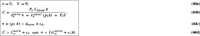
\(m\!\,=\!\,0,\quad e\!\,=\!\,0,\quad V\!\,=\!\,0,\quad n\!\,=\,n^{*},\quad b\!\,=\!\,b^{*} \text { such that}\)
\(n^{*}\!\,+\!\,(p_{1}\;b^{*})\!\,>d_{norm}+\epsilon _{d},\quad C\!\,=\!\,\dfrac{P_{c}\;C_{blood}\;b^{*}}{k^{norm}_{c}\;n^{*}\;+\;k^{vessel}_{c}\;(p_{1}b^{*})\;+\;P_{c}b^{*}}, \text { and} C >C_{v}^{norm}+\epsilon _{v}.\)
A non-trivial steady state representing a tissue with normal cells, blood vessels and oxygen. The sum of normal cell density and vessel density exceeds the carrying capacity for normal cells thus blocking normal cell proliferation. Also the vessel density is such that it supplies enough oxygen (\(C>C_{v}^{norm}+\epsilon _{v}>C_{a}^{norm}+\epsilon _{a}\)), so that there is no normal cell death, no VEGF production, and hence no angiogenesis.
-
4.
\(m\!\,=\!\,0,\quad e\!\,=\!\,0,\quad n\!\,=\,n^{*},\quad b\!\,=\!\,b^{*} \text { such that } n^{*}\!\,+\!\,(p_{1}\;b^{*})\!\,>d_{tip}+\epsilon _{d}, V\!\,=\!\,\dfrac{k_{v}^{norm}\;n^{*}}{P_{v}\;b^{*}\;+\;\delta _{v}},\quad C\!\,=\!\,\dfrac{P_{c}\;C_{blood}\;b^{*}}{k^{norm}_{c}\;n^{*}\;+\;k^{vessel}_{c}\;(p_{1}\;b^{*})\;+\;P_{c}\;b^{*}},\text { and} C_{a}^{norm}+\epsilon _{a}<C<C_{v}^{norm}+\epsilon _{v}.\)
This steady state, also non-trivial, represents a tissue with normal cells, blood vessels, oxygen and VEGF but no tip cells. Oxygen attains a certain level dictated by the blood vessel density and the normal cell density. This oxygen level, being below the threshold \(C_{v}^{norm}+\epsilon _{v}\), causes hypoxic normal cells to secrete VEGF. However, the normal cells and the blood vessels occupy the entire space in the tissue thus preventing any further sprouting from the blood vessels in response to the VEGF signals. Similar to the oxygen concentration, the VEGF concentration reaches a certain steady concentration depending on the normal cell density and the blood vessel density.
The non-trivial steady states suggest that n and b span a family of steady states such that \(n+(p_1 b) > d_{norm}+\epsilon _{d}\). The steady state oxygen concentration, given by Eq. (44b), is a function of the normal cell density and the blood vessel density. Tip cell densities are zero at steady state, and VEGF concentration is also zero in all cases, except when \(n+(p_1 b) > d_{tip}+\epsilon _{d}\) and \(C_{a}^{norm}+\epsilon _{a}<C<C_{v}^{norm}+\epsilon _{v}\).
To illustrate how different initial conditions lead to different steady states, we simulated the system of DAEs given by Eq. (33) in Appendix C, using the MATLAB routine ode15s, with different initial values of \(n \text { and } b\) and
for the parameter values given in Appendix A. The time-dependent solutions for each of these initial configurations projected on the (n, b) plane are shown in Fig. 6.

Course of the solutions of Eq. (33), projected on the (n, b) plane, for nine different initial configurations of \(n \text { and }b\) with \( m\!\,=\!\,0,\;e\!\,=\!\,0\) and \(C\text { and }V\) obtained from Eqs. (33a) and (33b), respectively. The red dashed line shows the trajectory starting at a for a value of \(\beta _{norm} = 1.66 \times 10^{-4},\) different from that in Table 2. The plane is divided into nine different regions defined by the thresholds for normal cell apoptosis, VEGF secretion, normal cell proliferation and tip cell production. The black line shows \(n+(p_1\;b)=d_{norm}\). The green line represents \(n=I(C_{a}^{norm})b\), and the blue line represents \(n=I(C_{v}^{norm})b\), where I(X) is as defined in Eq. (45). Dotted lines represent \(n=I(X \pm \epsilon _c)b\) where \(\epsilon _c\) is the length of the interval of smooth transitioning of the function given by Eq. (5) (Color figure online)

Temporal evolution, of all variables, along trajectory a as it traverses through the different regions shown in Fig. 6. Parameter values are given in Appendix A. Dashed line: mature tip cell density (Color figure online)
As seen from Fig. 6, the (n, b) space can be divided in nine different regions depending on the thresholds of oxygen for normal cell apoptosis and VEGF secretion and of total cell density for normal cell proliferation and tip cell production. In Fig. 7, we show the temporal evolution of all variables for trajectory a, which traverses the largest number of regions in Fig. 6.
We will now discuss how the path of the trajectory and hence the steady state configuration attained by the system varies for initial conditions lying in each of these regions.
- I :
-
Apoptosis, VEGF secretion - \(\mathbf {S_{tot}\!\,>d_{tip}+\epsilon _{d},\;C\!\,<C_{a}^{norm}+\epsilon _{a}}\)
The initial VEGF concentration is non-zero, since \(C\!\,<C_{a}^{norm}+\epsilon _{a}<C_{v}^{norm}+\epsilon _{v}\). However, since the total cell density exceeds the carrying capacity for tip cell sprouting, no new tips are formed. Normal cells undergo apoptosis due to hypoxia. Trajectories from this region (e.g. trajectories a and b) enter region II.
- II :
-
Apoptosis, VEGF secretion, angiogenesis - \(\mathbf {d_{norm}+\epsilon _{d}\!\,<S_{tot}\!\,<d_{tip}+\epsilon _{d},}\mathbf {C\!\,<C_{a}^{norm}+\epsilon _{a}}\)
In this region too, since \(C\!\,<\!\,C_{a}^{norm}+\epsilon _{a}\) initially, the normal cell density drops due to cell apoptosis. Tip cells are formed in response to VEGF. However, normal cells do not proliferate since the total cell density exceeds its carrying capacity. Depending on the vessel density, the trajectory enters region III (trajectory a) or V (trajectory b).
- III :
-
Apoptosis, proliferation, VEGF secretion, angiogenesis - \(\mathbf {S_{tot}\!\,<d_{norm}+\epsilon _{d},}\mathbf {C\!\,<C_{a}^{norm}+\epsilon _{a}}\)
Following trajectory a through this region, we see that the normal cell density continues to drop due to hypoxia. However, since the total cell density is less than the carrying capacity for tip cell sprouting, new tip cells form in response to VEGF. This leads to an increase in the blood vessel density followed by an increase in the oxygen concentration. This rise in oxygen and availability of space, since \(S_{tot}<d_{norm}+\epsilon _{d}\), promotes normal cell proliferation. Once the oxygen concentration rises beyond \(C_{a}^{norm}+\epsilon _{a}\), apoptosis stops and the trajectory enters region IV.
- IV :
-
Proliferation, VEGF secretion, angiogenesis - \(\mathbf {S_{tot}\!\,<d_{norm}+\epsilon _{d},}\) \(\mathbf {C_{a}^{norm}} \mathbf {+\,\epsilon _{a}\!\,<C<C_{v}^{norm}+\epsilon _{v}}\)
In this region, where \(C\!\,>C_{a}^{norm}+\epsilon _{a}\), there is no apoptosis and normal cells proliferate thus increasing the cell density. The cells also secrete VEGF since \(C\!\,<C_{v}^{norm}+\epsilon _{v}\). New tip cells are formed leading to an increase in the blood vessel density and thus oxygen concentration within the tissue. This rise in oxygen promotes further normal cell proliferation until \(S_{tot}\) crosses \(d_{norm}+\epsilon _{d}\). Trajectories from this region (e.g. trajectories a and d) enter region V
- V :
-
VEGF secretion, angiogenesis - \(\mathbf {d_{norm}+\epsilon _{d}\!\,<S_{tot}\!\,<d_{tip}+\epsilon _{d},}\) \(\mathbf {C_{a}^{norm}+\epsilon _{a}}\mathbf {<C\!\,<C_{v}^{norm}+\epsilon _{v}}\)
As seen from trajectory c and the continuation of trajectory a in this region, normal cells do not proliferate as the total density exceeds their carrying capacity. Since \(C\!\,<C_{v}^{norm}+\epsilon _{v}\), VEGF is secreted by the normal cells and new tip cells are formed leading to a further rise in blood vessel density and the oxygen concentration. This process continues until the oxygen concentration exceeds \(C_{v}^{norm}+\epsilon _{v}\), VEGF secretion stops, and the trajectory enters region VIII.
- VI :
-
VEGF secretion - \(\mathbf {S_{tot}\!\,>d_{tip}+\epsilon _{d},\;C_{a}^{norm}+\epsilon _{a}\!\,<C\!\,<C_{v}^{norm}+\epsilon _{v}}\)
For initial conditions in this region (e.g. trajectory g), there is enough oxygen for normal cells to survive since \(C>C_{a}^{norm}+\epsilon _{a}\). However, they do not proliferate due to lack of space. Thus the normal cell density remains unchanged. Normal cells secrete VEGF since \(C\!\,<C_{v}^{norm}+\epsilon _{v}\), but no new tip cells can be formed due to unavailability of space. Hence, new blood vessels cannot be formed and the blood vessel density also remains unchanged. All variables are in a steady state with non-zero VEGF concentration.
- VII :
-
Proliferation - \(\mathbf {S_{tot}\!\,<d_{norm}+\epsilon _{d},\;C\!\,>C_{v}^{norm}+\epsilon _{v}}\)
Since \(C\!\,>C_{v}^{norm}+\epsilon _{v}\!\,>C_{a}^{norm}+\epsilon _{a}\), normal cells do not secrete VEGF and do not undergo apoptosis. No VEGF implies the vessel density remains unchanged. However, normal cells proliferate and hence their cell density increases until \(S_{tot}\) crosses \(d_{norm}+\epsilon _{d}\), proliferation stops, and the trajectory (e.g. trajectory e) enters region VIII.
However, in cases like trajectory d with low blood vessel density and hence low oxygen concentration, the increase in consumption of oxygen, due to the increase in normal cell density, causes the oxygen concentration to drop below the threshold \(C_{v}^{norm}+\epsilon _{v}\). In this case, the trajectory traverses through regions IV and V before entering region VIII.
- VIII :
-
Steady state - \(\mathbf {d_{norm}+\epsilon _{d}\!\,<S_{tot}\!\,<d_{tip}+\epsilon _{d},\;C\!\,>C_{v}^{norm}+\epsilon _{v}}\)
In this region, normal cells do not proliferate due to lack of space. No VEGF is secreted by the normal cells since \(C\!\,>C_{v}^{norm}+\epsilon _{v}\). Hence, angiogenic sprouting does not occur. For initial conditions in this region (e.g. trajectory f), the variables are already in the steady state and hence the trajectory does not move at all.
For trajectories entering from region V or VII (e.g. trajectories a to e), the tip cells already present within the tissue continue to mature and form connections via anastomosis. Hence, the blood vessel density continues to rise until all the tip cells form connections. Once this process ends, all the variables attain a steady state and the trajectory stops.
- IX :
-
Steady state - \(\mathbf {S_{tot}\!\,>d_{tip}+\epsilon _{d},\;C\!\,>C_{v}^{norm}+\epsilon _{v}}\)
For initial conditions starting in this region (e.g. trajectory h), the variables are already in steady state since cells do not proliferate due to lack of space and also do not secrete VEGF or promote angiogenesis due to sufficient availability of oxygen. No trajectory starting in any other region can enter this region since it will eventually enter region VIII and attain a steady state as described earlier.
Since any initial configuration of \(n\text { and }b\) would lie in one of the nine regions mentioned above, the course of the solution will qualitatively follow the course of one of the trajectories shown in Fig. 6. However, it must be noted that the simulations in this section were performed with parameter values corresponding to the published multiscale model simulations as given in Appendix A. Changing the parameter values changes the behaviour of the system.
For instance, as seen from trajectory a, we see a rapid drop in the normal cell density. This is because the rate of normal cell death (\(\beta _{norm}=1\text { min}^{-1}\)) is much higher than the rate of tip cell sprouting \(\Big (P_{sprout}^{max}\dfrac{V}{V_{sprout}+V}=1.67 \times 10^{-4}\text { min}^{-1}\Big )\), with \(V=1\) nM, the typical VEGF concentration assumed in the model. For \(\beta _{norm}< P_{sprout}^{max}\dfrac{V}{V_{sprout}+V}\) trajectory a follows an altered path shown by the red dashed line in Fig. 6. In this case, because tip cells and eventually blood vessels are formed at a rate faster than normal cell apoptosis, the oxygen concentration rises beyond \(C_{a}^{norm}+\epsilon _{a}\) before trajectory a enters region III. As a result, trajectory a continues from region II into region V.
5 Wavespeed of Normal Tissue Expansion for Different Initial Conditions
We now seek for an estimate of the wavespeed of a travelling wave solution to Eq. (32) given in Appendix B. As \(x\rightarrow \infty \), we have \(n\rightarrow 0\) \(b\rightarrow b_{ss}\), \(C\rightarrow C_{ss}\), \(V\rightarrow 0\), \(e\rightarrow 0\) and \(m\rightarrow 0\). Linearising Eq. (32c) around this state, we obtain
Equation (22) is qualitatively similar to the Fisher-KPP equation, linearised at the leading edge, given as,
where \(\alpha \) is the growth rate and D is the diffusion coefficient.
Previous studies (Fisher 1937; McKean 1975; Mollison 1977; Larson 1978) have shown that Eq. (23) admits a travelling wave solution of the form \(u(x,t)=f(x-ct)\), for some function f, where c denotes the speed of the wave. Additionally, for initial conditions satisfying \(u=\mathscr {O}(e^{-\mu x})\) as \(x\rightarrow \infty \) the travelling wave evolves with a speed given as

By analogy with Eq. (24), we expect that a travelling wave whose normal cell density profile decays as \(e^{-\mu x}\) as \(x \rightarrow \infty \) has the approximate wavespeed
where
To test how the wavespeed for normal cell density varies with \(\mu \), the rate at which \(n\rightarrow 0\), we ran simulations with initial condition of normal cell density given as
where \(x_{0}=1\text { mm}\).
The blood vessel density was set to \(20\text { mm}^2/\text {mm}^3\) homogeneously, tip (immature and mature) cell density was zero. Solving Eqs. (32a) and (32b), at the leading edge of the wave where \(n_{ss}\rightarrow 0\), \(e_{ss}=m_{ss}=0\), and \(b_{ss}=20\), we get
Also note that at the leading edge, \(\mathscr {H}(d_{norm}-S_{tot}^{ss})=1\) since \(S_{tot}^{ss}=p_{1}b_{ss}<d_{norm}\).
Thus, by substituting C from Eq. (27a) in Eq. (25c), we can determine \(a_{\mu }\), \(a_{min}\) and \(\mu _{0}\), the value of \(\mu \) such that the wavespeed is minimum for \(\mu \ge \mu _{0}\).

Wave speed for the normal cell density obtained from Eq. (32) for initial conditions given in Eq. (26) for different values of the initial condition decay rate, \(\mu \). \(b=20\), \(e=m=0\). The simulated speed decreases with increasing \(\mu \) and attains the minimum speed when \(\mu \) crosses \(\sqrt{\dfrac{\alpha _{norm}(C_{ss})}{D_{norm}}}=38.7\) for \(C_{ss}\) given in Eq. (27a). Black circle: \(a_{\mu }\) given by Eq. (25a), the speed associated with the initial condition decay rate \(\mu \). Blue cross: \(a_{min}\), the predicted minimum speed given by Eq. (25b). Red cross: simulated wave speed (Color figure online)
As seen from the Fig. 8, for smaller values of \(\mu \), the simulated speed equals \(a_{\mu }\), given by Eq. (25a). However, as \(\mu \) exceeds \(\sqrt{\dfrac{\alpha _{norm}(C_{ss})}{D_{norm}}}=38.7\) for \(C_{ss}\) obtained from Eq. (27a), the normal cell density wave attains the minimum speed given by Eq. (25b).
Note that \(C_{ss}\) given by Eq. (27a) remains constant when \(e_{ss}=m_{ss}=0\), \(n_{ss}\rightarrow 0\) and \(b_{ss}\) is any arbitrary non-zero value less than \(d_{norm}\). Consequently, \(a_{norm}\) is constant for such a setup implying that the speed for normal cell density wave depends only on \(\mu \).
If the initial vessel density is such that \(p_1 b_{ss}\ge d_{norm}\), then \(C_{ss}\) is still given by Eq. (27a). However, \(a_{norm}\) will be zero since \(\mathscr {H}(d_{norm}-S_{tot}^{ss},\epsilon _{d})=0\) and \(\mathscr {H}(C_{a}^{norm}-C,\epsilon _{a})=0\). Thus, the normal cell density wave does not move in such a case. In our model simulations, we observe only a small change in the initial normal cell density profile owing to diffusion by random motility (result not shown).
6 Tumour Growth within a Normal Vascular Tissue
In this section, we perform simulations of a tumour tissue. Henceforth, we will use the term continuum model for the full system given by Eqs. (13), (14), (16), (17), (19) and (21).
To study tumour growth, we first simulate a well vascularised normal tissue, in the multiscale model, starting with the same setup described in Sect. 3. The initial and the final configuration (850 days) of the lattice is presented in Fig. 9a. Tumour cells are introduced to the final configuration and the simulation is continued, similar to simulations done in Owen et al. (2009, 2011).

Setup for simulation of tumour growth in a normal vascular tissue. a Top: initial normal tissue in the multiscale model consisting of one blood vessel surrounded by normal cells. Bottom: tumour cells introduced in the simulated well vascularised normal tissue. This configuration is used as initial condition for tumour growth simulation. Note that we ran 10 such realisations of a well vascularised normal tissue, which were then used as initial configurations for 10 realisations of the tumour growth simulation. b Density profiles of tumour cells, normal cells and blood vessel used for simulation of tumour growth in the continuum model. Red line: initial conditions for continuum model. Blue dashed lines: 1D profiles of 10 realisations of the well vascularised tumour tissue simulation of the multiscale model (one such shown in a), obtained by averaging in the y direction. Blue solid line: mean of the 1D profiles of 10 realisations of the multiscale model simulation (Color figure online)
In the continuum model, we set the normal cell density, homogeneously, equal to its carrying capacity, \(d_{norm}\), and the vessel density, homogeneously, to the average vessel density calculated from the multiscale model at the end of 850 days. No tip cells, mature or immature are present at the start of the simulation. All the parameter values are as defined in Appendix A. The density of tumour cells obtained from the multiscale model, by averaging in the y direction, is used as initial condition in the continuum model. The initial densities of tumour cells, normal cells and the blood vessels, in both the models, are presented in Fig. 9b.

Spatio-temporal evolution of normal and tumour cell densities from one realisation of the multiscale model simulation (left column) and the simulation of the continuum model (right column). The continuum model is able to well replicate the dynamics observed in the multiscale model. In both simulations, the tumour cells invade the healthy tissue by triggering normal cell apoptosis (Color figure online)
Figure 10 shows the spatio-temporal evolution of the normal and tumour cells. Tumour cells create a microenvironment that is hostile to normal cells and triggers their apoptosis. This creates space for tumour cell proliferation and invasion of the healthy tissue. In this particular simulation setup, the tissue is already sufficiently well vascularised to supply enough nutrients for tumour growth. Hence, no new vessels are formed.
6.1 Wavespeed of Tumour Invasion for Different Initial Conditions
The linearised form of Eq. (14) about the leading edge of the tumour invasion wave, where \(r\rightarrow 0\), \(n\rightarrow n_{ss}\), \(b\rightarrow b_{ss}\), \(C\rightarrow C_{ss}\), \(V \rightarrow 0\), \(e\rightarrow 0\), \(m\rightarrow 0\), (\(n_{ss}\), \(b_{ss}\) and \(C_{ss}\) are values attained by n, b and C as \(x\rightarrow \infty \)), is given by
Thus, as done for normal tissue expansion, the wave speed for tumour cell density with initial conditions that decay as \(e^{-\mu x}\) as \(x \rightarrow \infty \) is given by
where
To test how the initial condition decay rate, \(\mu \), affects the wave speed, we ran simulations for tumour invasion of a normal vascular tissue with initial tumour cell density given as
where \(x_{0}=1\) mm. Additionally, \(n(x,0)=d_{norm}\), \(b(x,0)=20\text { mm}^2/\text {mm}^3\), \(e(x,0)=m(x,0)=0\). Similar to normal tissue expansion, the oxygen and VEGF concentration at the leading edge of the tumour wave are given by
Also, \(\mathscr {H}(d_{tum}-S_{tot}^{ss},\epsilon _{d})=1\) since \(S_{tot}^{ss}<d_{tum}\). We can hence determine \(a_{tum}\), \(a_{\mu }^{tum}\), \(a_{min}^{tum}\) and \(\mu _{0}\), the value of \(\mu \) after which the tumour wave attains the minimum speed.
Figure 11 shows the tumour cell density wave speed for different values of \(\mu \). The simulated speed of the wave decreases with increasing \(\mu \). For \(\mu \) smaller than the threshold \(\sqrt{\frac{\alpha _{tum}(C)}{D_{tum}}}\), determined to be 35.2 for \(C_{ss}\) given by Eq. (31a), the wave speed equals \(a_{\mu }^{tum}\) given by Eq. (29a) and attains the predicted minimum speed, \(a_{min}^{tum}\) given by Eq. (29b) as \(\mu \) exceeds the threshold.
Unlike the case of normal tissue expansion, \(C_{ss}\), given by Eq. (31a), depends on the normal cell and vessel densities at the leading edge of the tumour cell density wave. Thus, the wave speed for tumour cell density depends not just on \(\mu \), the initial condition decay rate for tumour cell density, but also on the normal cell and vessel densities at the leading edge of the tumour wave. Thus, the speed of invasion of the normal tissue by the tumour cells depends on the configuration of the normal tissue.

Wave speed for the tumour cell density, obtained from the simulation of the continuum model for initial condition given in Eq. (30) for different values of initial condition decay rate \(\mu \). The simulated speed decreases with increasing \(\mu \). The simulated speed equals \(a_{\mu }^{tum}\) until it crosses the threshold \(\sqrt{\frac{\alpha _{tum}(C)}{D_{tum}}}\), determined for \(C_{ss}\) given by Eq. (27a). For \(\mu \) higher than the threshold, the simulated speed attains the predicted minimum speed, \(a_{min}^{tum}\). Black circles: \(a_{\mu }^{tum}\), given by Eq. (29a), the speed associated with initial condition decay rate, \(\mu \). Blue crosses: \(a_{min}^{tum}\) given by Eq. (29b) is the predicted minimum speed. Red crosses: simulated tumour cell density wave speed (Color figure online)
6.2 Dependence of Wavespeed on the Carrying Capacity of Tumour Cell Density
As mentioned in Sect. 6.1, the oxygen concentration at the leading edge of the tumour cell density wave does not depend on the densities of other model variables. Hence, the wave speed for tumour cell density given by Eq. (29), depends only on the decay rate, \(\mu \), and the availability of space given by \(\mathscr {H}(d_{tum}-S_{tot}^{ss},\epsilon _{d})\). For \(S_{tot}^{ss}\ge d_{tum}+\epsilon _{d}\), the minimum wave speed predicted by Eq. (29b) is zero. To determine the dependence of the wavespeed on the carrying capacity, we ran simulations of both the continuum and the multiscale models for different values of \(d_{tum}\). The initial conditions in the continuum model were as described in Sect. 6.1. We choose \(\mu =10^5\) since it approximates to the step function initial conditions used in the multiscale model and the wave associated with it attains the minimum speed.

Wave speed for the tumour cell density for different values of \(d_{tum}\) obtained as the mean of 10 realisations of the multiscale model (black circles) and from the simulation of the continuum model (red crosses). Blue crosses: minimum speed predicted from Eq. (29b). Green dashed line: \(S_{tot}^{ss}=d_{tum}+\epsilon _{d}\), the point of transition from pushed to pulled waves. For \(d_{tum}<S_{tot}^{ss}-\epsilon _{d}\), the tumour wave is a pushed wave since the speed of the tumour cell density wave depends on the whole wave front rather than the leading edge of the wave. Consequently, the (minimum) simulated speed of the wave is greater than the predicted minimum speed of zero (Color figure online)
As seen from Fig. 12, the wave speed decreases as the carrying capacity of the tumour cell density decreases (i.e. as \(d_{tum}-S_{tot}^{ss}\) decreases). Note that, for \(d_{tum}\le S_{tot}^{ss}+\epsilon _{d}\), the simulated speed is not equal to the predicted minimum speed of zero. Stokes (1976) refers to such waves as pushed waves since their speed of propagation is determined by the whole wave front and not by the leading edge, as in the case of pulled waves. In our model simulation, the tumour cells at the wave front create a hostile environment for the normal cells there, thus triggering their apoptosis. As the normal cells die, \(S_{tot}\) drops below \(d_{tum}+\epsilon _{d}\) consequently enabling tumour cell proliferation and progression of the wave. Thus, when \(S_{tot}>d_{tum}+\epsilon _{d}\), the speed of the wave for the tumour cell density does not depend on the leading edge of the wave but on the whole wave front of the tumour cell density.
7 Discussion
The focus of this work has been to develop a continuum model based on the multiscale model given in Owen et al. (2011) for growth of a vascular tumour tissue. Both the models account for evolution of normal and tumour cells and formation of vessels in response to surrounding conditions like availability of oxygen and secretion of VEGF. The results from the 1D continuum model were compared to the averaged density profiles obtained from a long 2D strip in the multiscale model. As seen from the density profiles in Figs. 4 and 10, the model results are qualitatively similar. However, in Fig. 4, the vessel density away from the parent vessel is low (5 \(\text { mm}^2/\text {mm}^3\)) in the continuum model compared to that in the multiscale model (20 \(\text { mm}^2/\text {mm}^3\)). One plausible reason for the difference in the vessel density could be the use of the snail-trail approach for movement of tip cells in the multiscale model. In this approach, it is assumed that the tip cells leave a trail of endothelial cells while moving within the tissue. On anastomosis, the entire trail forms a new vessel thus adding to the vessel density. We believe that we do not account for the snail-trail approach in the continuum model. However, we could extend the model to account for the snail-trail approach as done in Balding and McElwain (1985); Byrne and Chaplain (1995); Spill et al. (2015); Connor et al. (2015).
Moreover, not all processes from the multiscale models can be translated into rates in the continuum model. For instance, in the multiscale model, normal cell death and VEGF secretion depend on the intracellular p53 and VEGF concentration which evolve over time according to the local oxygen supply. We bypassed this subcellular dependence in the continuum model by assuming that the p53-VEGF subsystem attains a quasi-steady state, so the thresholds in terms of p53 and VEGF become thresholds in terms of local oxygen concentration. A parameter sensitivity analysis, where parameters in the continuum model, not directly taken from the multiscale model, are varied within physiological ranges, could provide additional information about the relative impact of individual parameters on the continuum model dynamics.
A drawback of the continuum model is that it is not clear how to include certain local dynamics like blood flow and adaptation of vessel radius to the microenvironment. However, with the continuum model, it was possible to analyse the steady states of the system, learn about wave speeds and their dependence on the model parameters and initial conditions. We determined that n and b span a family of steady states and showed that the steady state attained by the system depends on initial conditions of the model variables. As seen from Fig. 6, the \(n-b\) plane is divided into nine distinct regions by the thresholds of oxygen for normal cell apoptosis and VEGF secretion and of total cell density for normal cell proliferation and tip cell sprouting. Any initial condition for n and b will lie in one of these regions and thus qualitatively follow the course of the solutions shown in Fig. 6.
The system given by Eqs. (13), (14), (16), (17), (19) and (21) admits travelling waves for normal tissue expansion and tumour invasion into normal tissue. In the case of normal tissue expansion, the oxygen concentration at the leading edge of the wave remains constant for any non-zero value of the blood vessel density. Thus, the speed of the wave depends only on the decay rate of the initial profile of normal cell density. The wave for tumour invasion also depends on decay rate of the initial profile of tumour cell density. Additionally, it can be seen from Eq. (31a) that the oxygen concentration at the leading edge of the wave depends on the normal cell and vessel densities there. Thus, the speed at which the tumour invades a normal vascularised tissue depends on the configuration of that tissue. We also showed that the speed of the invading tumour wave varies with \(d_{tum}\), the threshold of total cell density for tumour cell proliferation and changes from a pulled to a pushed wave if \(d_{tum}\) is less than the total cell density at the leading edge of the wave. These pushed waves of tumour invasion propagate by creating a microenvironment that is hostile for normal cell survival, thus triggering apoptosis of normal cells at the wave front.
To the best of our knowledge, a model as complex as the multiscale model from Owen et al. (2011) has not been compared to an equivalent continuum model before. We remark that the focus of this paper was on the published multiscale model from Owen et al. (2011). However, it would be interesting to consider different models for the cell cycle, alternative rules for cell apoptosis and entry to/exit from quiescence, in the multiscale model and then correspondingly in the continuum model.
The multiscale model from Owen et al. (2011) also includes conventional drug therapy and a macrophage-based gene therapy. In the multiscale model, the chemotherapeutic drug is assumed to be a continuous variable and its evolution is given by Eq. (15). It would thus be straightforward to include a chemotherapeutic drug as an additional variable in the continuum model. Cells, in the multiscale model, with local drug concentration higher than a prescribed threshold intercalate the drug and die on attempting to divide. This effect of the drug on the cell densities in the continuum model can be modelled using \(\mathscr {H}\) given by Eq. (5). For the macrophage-based gene therapy in the multiscale model, macrophages are assumed to extravasate from the pre-existing blood vessels at a certain probability, similar to tip cell extravasation. Hence, as done for tip cell sprouting, we can readily model macrophage extravasation in the continuum model. The extended continuum model could then be used to analyse the impact of drug and macrophages on the speed of the tumour invasion wave. Such analysis might further help in designing novel therapeutic strategies to reduce the speed at which the tumour invades a normal vascularised tissue.
References
Alarcón T, Byrne H, Maini P (2003) A cellular automaton model for tumour growth in inhomogeneous environment. J Theor Biol 225(2):257–274
Alarcón T, Byrne HM, Maini PK (2004) A mathematical model of the effects of hypoxia on the cell-cycle of normal and cancer cells. J Theor Biol 229(3):395–411
Alarcón T, Byrne HM, Maini PK (2005) A multiple scale model for tumor growth. Multiscale Model Simul 3(2):440–475
Alarcón T, Owen MR, Byrne HM, Maini PK (2006) Multiscale modelling of tumour growth and therapy: the influence of vessel normalisation on chemotherapy. Comput Math Methods Med 7(2–3):85–119
Anderson A, Rejniak K, Gerlee P, Quaranta V (2007) Modelling of cancer growth, evolution and invasion: bridging scales and models. Math Model Nat Phenom 2(3):1–29
Aubert M, Chaplain MAJ, McDougall SR, Devlin A, Mitchell CA (2011) A continuum mathematical model of the developing murine retinal vasculature. Bull Math Biol 73(10):2430–2451
Balding D, McElwain DLS (1985) A mathematical model of tumour-induced capillary growth. J Theor Biol 114(1):53–73
Betteridge R, Owen MR, Byrne HM, Alarcón T, Maini PK (2006) The impact of cell crowding and active cell movement on vascular tumour growth. Netw Heterog Media 1(4):515–535
Byrne HM, Chaplain MAJ (1995) Mathematical models for tumour angiogenesis: numerical simulations and nonlinear wave solutions. Bull Math Biol 57(3):461–486
Byrne HM, Chaplain MAJ (1998) Necrosis and apoptosis: distinct cell loss mechanisms in a mathematical model of avascular tumour growth. Comput Math Methods Med 1(3):223–235
Chaplain MAJ, Stuart AM (1991) A mathematical model for the diffusion of tumour angiogenesis factor into the surrounding host tissue. Math Med Biol 8(3):191–220
Connor AJ, Nowak RP, Lorenzon E, Thomas M, Herting F, Hoert S, Quaiser T, Shochat E, Pitt-Francis J, Cooper J et al (2015) An integrated approach to quantitative modelling in angiogenesis research. J R Soc Interface 12(110):20150–20546
Edelstein-Keshet L, Ermentrout B (1989) Models for branching networks in two dimensions. SIAM J Appl Math 49(4):1136–1157
Fisher RA (1937) The wave of advance of advantageous genes. Ann Eugen 7(4):355–369
Gaffney EA, Pugh K, Maini PK, Arnold F (2002) Investigating a simple model of cutaneous wound healing angiogenesis. J Math Biol 45(4):337–374
Gatenby RA, Gawlinski E (2001) Mathematical models of tumour invasion mediated by transformation-induced alteration of microenvironmental ph. In: Novartis foundation symposium, vol 1999. Wiley, Chichester, New York, pp 85–95
Larson DA (1978) Transient bounds and time-asymptotic behavior of solutions to nonlinear equations of fisher type. SIAM J Appl Math 34(1):93–104
McKean HP (1975) Application of brownian motion to the equation of Kolmogorov–Petrovskii–Piskunov. Commun Pure Appl Math 28(3):323–331
Mollison D (1977) Spatial contact models for ecological and epidemic spread. J R Stat Soc Ser B (Methodol) 39(3):283–326
Owen MR, Alarcón T, Maini PK, Byrne HM (2009) Angiogenesis and vascular remodelling in normal and cancerous tissues. J Math Biol 58:689–721
Owen MR, Stamper IJ, Muthana M, Richardson GW, Dobson J, Lewis CE, Byrne HM (2011) Mathematical modeling predicts synergistic antitumor effects of combining a macrophage-based, hypoxia-targeted gene therapy with chemotherapy. Cancer Res 71:2826–2837
Painter KJ, Hillen T (2002) Volume-filling and quorum-sensing in models for chemosensitive movement. Can Appl Math Q 10(4):501–543
Perfahl H, Byrne HM, Chen T, Estrella V, Alarcón T, Lapin A, Gatenby RA, Gillies RJ, Lloyd MC, Maini PK, Reuss M, Owen MR (2011) Multiscale modelling of vascular tumour growth in 3d: the roles of domain size and boundary conditions. PLoS ONE 6(4):e14,790
Ribba B, Colin T, Schnell S (2006) A multiscale mathematical model of cancer, and its use in analyzing irradiation therapies. Theor Biol Med Model 3(1):1
Royds J, Dower S, Qwarnstrom E, Lewis C (1998) Response of tumour cells to hypoxia: role of p53 and nfkb. Mol Pathol 51(2):55
Schnepf A, Roose T, Schweiger P (2008) Impact of growth and uptake patterns of arbuscular mycorrhizal fungi on plant phosphorus uptake—a modelling study. Plant Soil 312(1):85–99
Spill F, Guerrero P, Alarcon T, Maini PK, Byrne HM (2015) Mesoscopic and continuum modelling of angiogenesis. J Math Biol 70(3):485–532
Stokes AN (1976) On two types of moving front in quasilinear diffusion. Math Biosci 31(3):307–315
Stolarska MA, Kim Y, Othmer HG (2009) Multi-scale models of cell and tissue dynamics. Philos Trans R Soc Lond A Math Phys Eng Sci 367(1902):3525–3553
Author information
Authors and Affiliations
Corresponding author
Appendices
Appendix A Parameter Values
In the multiscale model by Owen et al. (2011), a lattice site corresponds to a cube with length of each side equal to \({\varDelta }x=40\mu \text {m}=0.04\text { mm}\). Let us denote the volume of one lattice site by \(V_{site}=6.4\times 10^{-5}\text { mm}^3\). For the remainder of this section, lattice site has the same meaning as above unless stated otherwise.
1.1 Estimation of \(P_{c}\)
We ran simulations of the multiscale model for different vessel densities on a \(1\times 1\) square lattice with only one normal cell. The simulations were run only for one time step, and the oxygen concentration was noted. Since the lattice dimensions are \(1\times 1\), we can assume that the system is spatially homogeneous and thus obtain \(P_{c}\) by substituting the values of n, b and C in Eq. (16). The value is given in Table 3.
1.2 Estimation of \(k^{cell}_{c}\), \(k^{cell}_{v}\)
In the multiscale model, for one cell in one lattice site, the rate of oxygen consumption by cell type cell, \(k^{cell}_{c}\) \(\text {min}^{-1}\), represents the rate of consumption for one cell per \(V_{site}\).
Therefore, to obtain the rate in units of per cell density per min (\({(\text {cell}/\text {mm}^{3})}^{-1} \text {min}^{-1}\)), suitable for the continuum model, we multiply \(k^{cell}_{c}\) by \(V_{site}\).
The rate of VEGF secretion by cell type cell, \(k^{cell}_{v}\), is also obtained similarly. The values used in the continuum model are given in Table 2.
1.3 Estimation of \(d_{cell}\)
In the multiscale model, the carrying capacity of a cell at lattice site x is defined as the maximum number of cells that can be present at x. Therefore, we obtain the carrying capacity for the continuum model as number of cells per unit volume (\(\text {cells}/\text {mm}^3\)) by dividing the carrying capacity by \(V_{site}\). The value is given in Table 2.
1.4 Estimation of \(D_{cell}\)
In the multiscale model, apart from random movement, normal and tumour cells also spread by via cell division by placing their daughter cells in neighbouring sites if the number of cells in the parent cell’s site exceeds its carrying capacity. A cell of type cell takes at least \(T_{min}^{cell}\) minutes to divide. On division, the new cell is placed in one of Moore neighbourhood sites. Thus, the mean squared displacement of the cell in \(T_{min}^{cell}\) min is of the order of \({\varDelta }x\) mm.
For normal cells, the random motility coefficient, in the multiscale model, is zero. We thus estimate the value of \(D_{norm}\) using the mean squared displacement estimated above. For tumour cells, the random motility coefficient in the multiscale model is non-zero. Thus, starting with the estimate obtained from the mean squared displacement of tumour cells, we simulate the continuum model for different values of \(D_{tum}\) and compare the distance covered in unit time with the simulation from the multiscale model. The best fit thus obtained was chosen as the value for \(D_{tum}\).
All the values of \(D_{cell}\) are given in Table 4.
1.5 Estimation of \(p_{1}\)
In all simulations of the multiscale model presented in this paper, all vessels have a fixed radius \(R = 0.006 \text { mm}\) and typical length \(L={\varDelta }x\). Also, in the multiscale model, all blood vessels in a lattice site are associated with one endothelial cell. Therefore, in a lattice site with volume \(V_{site}\), each vessel with surface density of \(2\pi R {\varDelta }x/V_{site}=23.56\text { mm}^{2}/\text {mm}^{3}\) has an endothelial cell density of \(1/V_{site}=15{,}625\text { cells}/\text {mm}^3\) associated with it. Therefore, \(p_{1}\), defined as the number of endothelial cells per unit vascular surface area is obtained by dividing the endothelial cell density by the vessel surface density. Thus \(p_{1}=663\) cells/mm\(^2\), as given in Table 5.
1.6 Estimation of \(\lambda _{2}\)
Estimating the rates of tip-tip and tip-vessel anastomosis from the multiscale model is difficult. We thus use the values given in Schnepf et al. (2008). To convert \(\overline{\lambda _2}\) from units of per unit capillary length density per unit time to the units of per unit capillary surface density per unit time, we multiply \(\overline{\lambda _{2}}\) from Schnepf et al. (2008) with the surface area of a vessel with radius \(0.006\text { mm}\) and unit length. The values of \(\lambda _1\) and \(\lambda _2\) are given in Table 5.
Appendix B Normal Vasculature Tissue Model
Oxygen
VEGF
Normal Cell Density
Immature Tip Cell Density
Mature Tip Cell Density
Blood Vessel Density
Appendix C Steady State Analysis
Assuming all the variables to be spatially homogeneous, we obtain the following set of differential algebraic equations (DAEs),
To determine the steady states of Eq. (33), we set \(\hbox {d}/\hbox {d}t=0\) for all variables.
Equation (33f) holds only if \(m\!\,=\!\,0\). Substituting \(m\!\,=\!\,0\) in Eq. (33e) gives
implying \(e\!\,=\!\,0\). Substituting \(e\!\,=\!\,0\) in Eq. (33d) gives
Note In the remainder of this section, \(S_{tot}=n+(p_1\!\,b)\), since \(e=0\) and \(m=0\).
Equation (35) holds if, either
-
\(b = 0, \text { or }\)
-
\(\dfrac{V}{V_{sprout}+V}=0 \implies V=0, \text{ or } \)
-
\(\mathscr {H}(d_{tip}-S_{tot},\epsilon _{d})=0 \implies S_{tot} > d_{tip}+\epsilon _{d}\),
where \(\mathscr {H}(z,\epsilon )\) is as defined in Eq. (5). The smoothness of transition from 0 to 1 is given by the value of \(\epsilon \). As the value of the function is zero for \(z\le -\epsilon \), steady state will only be attained when \(z \le -\epsilon \). For \(\epsilon =0\), the function reduces to the discontinuous Heaviside function reflecting the dynamics observed in the multiscale model.
We now analyse the possible cases leading to steady states of Eq. (33).
- Case 1 :
-
Let us assume that \(b\!\,=\!\,0\). Substituting the values of \(e \text { and } b\) in Eq. (33a) gives
$$\begin{aligned} k^{norm}_{c}\;n\;C\!\,=\!\,0. \end{aligned}$$(36)Equation (36) is satisfied if either \(n\!\,=\!\,0 \text { or } C\!\,=\!\,0\).
- Case 1.1 :
-
If \(n\!\,=\!\,0\), then \(C\!\,=\!\,C^{*}\), where \(C^{*}\) is arbitrary, satisfies Eq. (36). Also, Eq. (33b) becomes \(\delta _{v}V=0\) which implies \(V\!\,=\!\,0\). Thus, the first possible steady state configuration is
$$\begin{aligned} \boxed {m\!\,=\!\,0,\quad e\!\,=\!\,0,\quad V\!\,=\!\,0,\quad n\!\,=\!\,0,\quad b\!\,=\!\,0,\quad C\!\,=\!\,C^{*}.} \end{aligned}$$(37)This steady state represents a tissue with no cells and no blood vessels and an arbitrary oxygen concentration.
- Case 1.2 :
-
If \(C\!\,=\!\,0\), Eq. (33c) reduces to \(\beta _{norm}\;n\!\,=\!\,0\) which implies \(n=0\) which further implies \(V=0\) as in Case 1.1. Thus we have
$$\begin{aligned} \boxed {m\!\,=\!\,0,\quad e\!\,=\!\,0,\quad V\!\,=\!\,0,\quad n\!\,=\!\,0,\quad b\!\,=\!\,0,\quad C\!\,=\!\,0.} \end{aligned}$$(38)This state is thus a special case of Case 1.1 representing a tissue with no cells, no blood vessels and no oxygen.
- Case 2 :
-
When \(V\!\,=\!\,0\), Eq. (33b) reduces to
$$\begin{aligned} \mathscr {H}(C_{v}^{norm}-C,\epsilon _{v})\;k_{v}^{norm}\;n\;=\;0. \end{aligned}$$(39)It must be noted that we have assumed \(V_{blood}=0\). This leads to two possibilities, either \(C\!\,>C_{v}^{norm}+\epsilon _{v}\) or \(n\!\,=\!\,0\).
- Case 2.1 :
-
If \(n\!\,=\!\,0\), Eq. (33a) becomes
$$\begin{aligned} P_{c}\;b\;(C_{blood}-C)\!\,-\!\,k^{vessel}_{c}\;(p_{1}\;b)\;C\!\,=\!\,0, \end{aligned}$$(40)which implies \(C=\dfrac{P_{c}\;C_{blood}}{k^{vessel}_{c}\;p_{1}\;+\;P_{c}}\). Also \(n\!\,=\!\,0\) satisfies Eq. (33c). Thus, the next possible steady state configuration is given by
$$\begin{aligned} \boxed {m\!\,=\!\,0,\quad e\!\,=\!\,0,\quad V\!\,=\!\,0,\quad n\!\,=\!\,0,\quad b\!\,=\!\,b^{*}>0,\quad C\!\,=\!\,\dfrac{P_{c}\;C_{blood}}{k^{vessel}_{c}\;p_{1}\,\!+\,\!P_{c}}.} \end{aligned}$$(41)This represents a tissue with only blood vessels of arbitrary density, \(b^{*}>0\) and oxygen supplied and consumed by those vessels.
- Case 2.2 :
-
Let us now consider the other possibility, \(C\!\,>C_{v}^{norm}+\epsilon _{v}\). Since \(C_{v}^{norm}+\epsilon _{v}\!\,>C_{a}^{norm}+\epsilon _{a}\), we have \(C>C_{v}^{norm}+\epsilon _{v}>C_{a}^{norm}+\epsilon _{a}\). Hence, Eq. (33c) reduces to
$$\begin{aligned} \dfrac{\ln (2)}{T_{min}^{norm}}\dfrac{C}{C_{\phi }^{norm}+C}\mathscr {H}(d_{norm}-S_{tot},\epsilon _{d})n=0. \end{aligned}$$(42)For Eq. (42) to be true, either \(n\!\,=\!\,0 \text { or } S_{tot}\!\,>d_{norm}+\epsilon _{d}\).
- Case 2.2.1 :
-
Let \(n\!\,=\!\,0\). This leads us back to Case 2.1, implying that the steady state configuration is given by Eq. (41).
Although for the given parameter set, \(C\!\,=\!\,\dfrac{P_{c}\;C_{blood}}{k^{vessel}_{c}\;p_{1}\;+\;P_{c}}\;>C_{v}^{norm}+\epsilon _{v}\) holds, the inequality is irrelevant in this case because, irrespective of the oxygen concentration, there will be no VEGF production in the absence of normal cells (\(n\!\,=\!\,0\)).
- Case 2.2.2 :
-
Next, let us assume, \(S_{tot}\!\,=n\!\,+\!\,(p_{1}\;b)\!\,>d_{norm}+\epsilon _{d}\). From Eq. (33a) we get,
$$\begin{aligned} P_{c}\;b\;(C_{blood}-C)\!\,-\!\,k^{norm}_{c}\;n\;C\!\,-\!\,k^{vessel}_{c}\;(p_{1}\;b)\;C\!\,=\!\,0. \end{aligned}$$(43)Thus, another possible steady state configuration is given by
where
$$\begin{aligned} I(X)\;=\;\dfrac{P_{c}\;C_{blood}\;-\;X\;k^{vessel}_{c}\;p_{1}\;-\;X\;P_{c}}{X\;k^{norm}_{c}}. \end{aligned}$$(45)This state represents a tissue with normal cells, blood vessels and oxygen. The sum of normal cell density and vessel density exceeds the carrying capacity for normal cells thus blocking normal cell proliferation. Also the vessel density is such that it supplies enough oxygen (\(C>C_{v}^{norm}+\epsilon _{v}>C_{a}^{norm}+\epsilon _{a}\)), so that there is no normal cell death and no VEGF production leading to angiogenesis.
- Case 3 :
-
In this case, \(S_{tot}\!\,=n\!\,+\!\,(p_{1}\;b)\!\,>d_{tip}+\epsilon _{d}\). Since \(d_{tip}+\epsilon _{d}\!\,>d_{norm}+\epsilon _{d}\), Eq. (33c) reduces to
$$\begin{aligned} \mathscr {H}(C_{a}^{norm}-C,\;\epsilon _{a})\;\beta _{norm}\;n\!\,=\!\,0, \end{aligned}$$which holds either if \(n\!\,=\!\,0 \text { or } C\!\,>C_{a}^{norm}+\epsilon _{a}\).
- Case 3.1 :
-
Let \(n\!\,=\!\,0\). Equation (33b) reduces to \(\delta _{v}V\!\,=\!\,0\) implying \(V\!\,=\!\,0\). These conditions lead to the steady state configuration given in Case 2.1 with an added condition, \(S_{tot} = p_{1}b > d_{tip}+\epsilon _{d}\). However, \(V=0\) satisfies Eq. (33d) irrespective of the value of \(S_{tot}\). Hence, the extra condition is irrelevant.
- Case 3.2 :
-
Let \(C\!\,>C_{a}^{norm}+\epsilon _{a}\). From Eq. (43), we get
$$\begin{aligned} C\!\,=\!\,\dfrac{P_{c}\;C_{blood}\;b}{k^{norm}_{c}\;n\;+\;k^{vessel}_{c}\;(p_{1}\;b)\;+\;P_{c}\;b}. \end{aligned}$$Rearranging the inequality \(C>C_{a}^{norm}+\epsilon _{a}\), we can obtain a relation between n and b, as follows,
$$\begin{aligned} n < I(C_{a}^{norm}+\epsilon _{a}) b, \end{aligned}$$(46)where \(I(C_{a}^{norm}+\epsilon _{a})\) is defined in Eq. (45). Also, from Eq. (33b), we obtain
$$\begin{aligned} V\!\,=\!\,\dfrac{\mathscr {H}(C_{v}^{norm}-C,\epsilon _{v})\;k_{v}^{norm}\;n}{P_{v}\;b\;+\;\delta _{v}}. \end{aligned}$$(47) - Case 3.2.1 :
-
Thus, if \(C\!\,>C_{v}^{norm}+\epsilon _{v}\), the steady state configuration becomes
$$\begin{aligned}&e\!\,=\!\,0,\quad V\!\,=\!\,0, \end{aligned}$$(48a)$$\begin{aligned}&C\!\,=\!\,\dfrac{P_{c}\;C_{blood}\;b}{k^{norm}_{c}\;n\;+\;k^{vessel}_{c}\;(p_{1}\;b)\;+\;P_{c}\;b}, \end{aligned}$$(48b)$$\begin{aligned}&n\!\,+\!\,(p_{1}\;b)\!\,>d_{tip}+\epsilon _{d}, \end{aligned}$$(48c)$$\begin{aligned}&C\!\,>C_{v}^{norm}+\epsilon _{v}\implies n\!\,<\!\,I(C_{v}^{norm}+\epsilon _{v})\;b, \end{aligned}$$(48d)where I(X) is defined in Eq. (45).
However, it is worth noting that when \(e=0 \text { and } C>C_{v}^{norm}+\epsilon _{v}\), Eq. (33d) holds irrespective of \(S_{tot}=n+(p_{1}b)>d_{tip}+\epsilon _{d}\). Hence, the condition given in Eq. (48c) is irrelevant. However, on omitting this condition, Eq. (33c) holds either if \(n=0\), which leads to Case 2.1, or if \(S_{tot}=n+(p_{1}b)>d_{norm}+\epsilon _{d}\), which leads to Case 2.2.2. Thus, the configuration obtained in Eq. (48) is not a new configuration.
- Case 3.2.2 :
-
Next, when \(C\!\,<C_{v}^{norm}+\epsilon _{v}\), we get
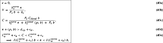
where I(X) is defined in Eq. (45).
This steady state represents a tissue with normal cells, blood vessels, oxygen and VEGF but no tip cells. The oxygen attains a certain concentration dictated by the blood vessel density and the normal cell density. This value of the concentration being below the threshold \(C_{v}^{norm}+\epsilon _{v}\), causes hypoxic normal cells to secrete VEGF. However, the normal cells and the blood vessels occupy the entire space in the tissue thus preventing any further sprouting from the blood vessels in response to the VEGF signals. Similar to the oxygen concentration, the VEGF concentration reaches a certain steady concentration depending on the normal cell density and the blood vessel density.


Rights and permissions
About this article

Cite this article
Joshi, T.V., Avitabile, D. & Owen, M.R. Capturing the Dynamics of a Hybrid Multiscale Cancer Model with a Continuum Model. Bull Math Biol 80, 1435–1475 (2018). https://doi.org/10.1007/s11538-018-0406-6
Received:
Accepted:
Published:
Issue Date:
DOI: https://doi.org/10.1007/s11538-018-0406-6