
Abstract
We show that when selection is extreme—the fittest strategy always reproduces or is imitated—the unequivalence between the possible evolutionary game scenarios in finite and infinite populations resolves, in the sense that the three generic outcomes—dominance, coexistence, and mutual exclusion—emerge in well-mixed populations of any size. We consider the simplest setting of a 2-player-2-strategy symmetric game and the two most common microscopic definitions of strategy spreading—the frequency-dependent Moran process and the imitation process by pairwise comparison—both in the case allowing any intensity of selection. We show that of the seven different invasion and fixation scenarios that are generically possible in finite populations—fixation being more or less likely to occur and rapid compared to the neutral game—the three that are possible in large populations are the same three that occur for sufficiently strong selection: (1) invasion and fast fixation of one strategy; (2) mutual invasion and slow fixation of one strategy; (3) no invasion and no fixation. Moreover (and interestingly), in the limit of extreme selection 2 becomes mutual invasion and no fixation, a case not possible for finite intensity of selection that better corresponds to the deterministic case of coexistence. In the extreme selection limit, we also derive the large population deterministic limit of the two considered stochastic processes.
1 Introduction
Evolutionary game theory (Maynard Smith and Price 1973; Taylor and Jonker 1978; Maynard Smith 1982; Hofbauer and Sigmund 1998) is the standard approach to describe the spreading of different strategies under frequency-dependent selection—the fitness or reproductive output of a strategy depending on the type and frequency of its competitors. In the deterministic limit of large and well-mixed populations, the dynamics of the frequencies is described by the well-known replicator equation (Taylor and Jonker 1978; Maynard Smith 1982; Hofbauer and Sigmund 1998). Games are however played within finite groups, and this motivated the stochastic modeling of games in finite populations (Nowak 2006), with the introduction of two common microscopic mechanisms of strategy spreading: the frequency-dependent Moran process (Nowak et al. 2004; Taylor et al. 2004) and the pairwise comparison of the expected payoffs (Traulsen et al. 2005, 2006, 2007), i.e., spreading by reproduction and imitation of the fittest, respectively.
Though both mechanisms lead to the standard (or adjusted) replicator dynamics in the large population limit (Traulsen et al. 2005), the results for finite populations turned out to be possibly very different from the corresponding deterministic limit. For example, among two alternative strategies A and B, strategy A could dominate B in medium-size populations, while B dominates A in the same game replicator dynamics (Taylor et al. 2004). Moreover, competition scenarios that do not match with any of the deterministic cases can occur within finite groups, e.g., scenarios of mutual invasion in which one strategy has high chances to replace the other after invasion.
To compare evolutionary game dynamics in finite and infinite populations, the notions of invasion and replacement after invasion—fixation—have been consistently defined for the stochastic processes describing the spreading of strategies in finite populations (Nowak 2006). Specifically for two-strategy games (Taylor et al. 2004, 2006; Antal and Scheuring 2006), strategy A invades B if the transition probability from 1 to 2 A-individuals is higher than that from 1 to 0, whereas fixation is defined using the neutral game—the totally random game with equal expected payoffs for A and B—as benchmark. That is, A is shortly said to fixate in a population of N individuals if the chances to go from 1 to N A-strategists—the fixation probability for A—are more compared to the N-individual neutral game. Moreover, fixation is said to be fast or slow if the expected number of transitions to fixate—the fixation time—is smaller or larger compared to the neutral game. Of course, by “A invades B” and “A fixates” we do not mean that invasion and fixation necessarily occur. We can only say that they are favored by selection, in the sense that the chances to invade/fixate are more than in the absence of a selection mechanism. Specifically for fixation, note that when the fixation of one strategy is favored by selection, this is so compared to the neutral game, not against the other strategy. According to this notation, selection could thus favor the fixation of both strategies.
The above definitions of invasion and fixation induce a classification of 2-strategy games in finite populations. Considering only the generic situations (i.e., neglecting the game classes—some of which are interesting—that have zero measure in the set of all possible games), there are 12 qualitatively different types of games, summarized in Table 1, depending on whether A/B invades B/A, A and B fixate or not, and fixation is fast or slow. And the number of classes reduces to 7 if symmetric situations under the interchange of A and B are grouped together. Evidently, not all combinations of invasion and fixation are possible and this was shown by Taylor et al. (2004) (for the invasion and fixation probabilities) and by Antal and Scheuring (2006) (for the fixation time) for the Moran process with linear fitness. In the simplest setting of 2-player-2-strategy symmetric games [as in Taylor et al. (2004) and Antal and Scheuring (2006)], we show that the same classification holds for the Moran process with exponential fitness and for the pairwise comparison process with exponential formulation of the imitation probability—two models later introduced to allow any intensity of selection (see, e.g., Traulsen et al. (2006, 2007, 2008), respectively).
Note that, among the seven generic cases, the first three qualitatively correspond to the generic behaviors of the 2-strategy replicator equation—dominance, coexistence, and mutual exclusion, respectively. And indeed any generic game falls into classes 1–3 when played within a sufficiently large group. This was also shown by Taylor et al. (2004) and Antal and Scheuring (2006) for the Moran process with linear fitness, and it is here extended to the Moran and pairwise comparison processes allowing any intensity of selection.
The main result of this paper is that the same three classes of games are the only possible when selection is sufficiently strong. This somehow unifies evolutionary game dynamics in finite and infinite populations. The same game (same payoffs) can however fall into different classes (among 1–3) if played within a large group with mild selection or within a small group with strong selection. Obviously, the classes come to coincide if selection intensity is increased in the first case and population size in the second.
We also show that, in the limit of extreme selection, class 2 becomes “mutual invasion and no (slow) fixation” (

), since for both strategies the probability to go extinct drops to zero in the limit. Indeed, when selection is extreme under mutual invasion, both strategies always reproduce in the Moran process and are always copied in the pairwise comparison when represented by one (or a few) individuals. Note that this new case is not possible for finite intensity of selection but, interestingly, it better corresponds to the deterministic case of coexistence than “mutual invasion and slow fixation of one strategy.” In fact, in a case of coexistence, one would expect the fixation of a strategy to be less likely to occur than in a totally random game. However, as long as the intensity of selection is finite, this is not the case for one strategy, though fixation becomes slower and slower while increasing the strength of selection and this allows the longer and longer coexistence of the two strategies. As we show in Sect. 2.4, while increasing the strength of selection, the fixation probability approaches one for the strategy most represented at coexistence and vanishes for the other. However, both probabilities drop to zero in the limit.
The paper is organized as follows. In Sects. 2.1 and 2.2 we review the two considered mechanisms of strategy spreading, and we formulate the results that show the classification in Table 1 (proofs are reported in “Appendix”). In Sects. 2.3 and 2.4 we refine the classification, respectively, showing that only games of classes 1–3 are generically possible in large populations and for strong selection. We also consider the limit to extreme selection in Sect. 2.4 and derive the large-population-extreme selection deterministic limit of the two considered stochastic processes. Then, in Sect. 2.5 we numerically evaluate the trade-off between population size and intensity of selection in ruling out classes 4–7. Our finding is further discussed and generalized in Sect. 3.
2 Methods
2.1 2-Player-2-Strategy Symmetric Games in Finite Populations
The game is played by two participants—the players—randomly selected from a population of N individuals, i of which adopt strategy A, the remaining \(N-i\) adopting strategy B. According to the payoff matrix

the expected payoffs for the A- and B-strategists are
The spreading of the two strategies is modeled as a random walk through the states \(i=0,1,\ldots ,N\) of the Markov chain in Fig. 1. We consider the following two mechanisms of strategy transmission from one individual to another.

The Markov chain governing the evolutionary dynamics (\(N>3\))
-
The frequency-dependent Moran process (Nowak et al. 2004; Taylor et al. 2004). It is the birth–death process at each transition of which one individual is selected for reproduction with probability proportional to its fitness and one individual is randomly removed from the population. The fitness is a nonnegative measure of individual performance in the underlying game. It can be simply taken equal to the expected payoffs for games with nonnegative payoffs (Taylor et al. 2004) or, more generally, increasing with the payoff (Wu et al. 2010). To discuss the role of selection, the convex combination of a baseline fitness and the payoff has been often used (Nowak et al. 2004), the weight of the combination measuring the strength of selection. This formulation however limits the strength of selection to 1 [the case referred to as strong selection in Fudenberg et al. (2006)], and more stringent upper bounds are imposed if payoffs are allowed to be negative (Traulsen and Hauert 2009). To avoid this restriction and allow any strength of selection, we use the exponential fitness formulation proposed in Traulsen et al. (2008)
$$\begin{aligned} f_{A,i}=\exp (s\pi _{A,i})\quad \text {and}\quad f_{B,i}=\exp (s\pi _{B,i}), \end{aligned}$$(2)where s is hereafter called intensity of selection. Modulating s from 0 to \(\infty \), we describe processes from neutral drift (all individuals reproduce with equal probability) to extreme selection (the best performing strategy always reproduces). The transition probabilities of the Markov chain are
$$\begin{aligned} T^+_i=\displaystyle \frac{\displaystyle if_{A,i}}{\displaystyle if_{A,i}+(N-i)f_{B,i}}\displaystyle \frac{\displaystyle N-i}{\displaystyle N}\quad \text {and}\quad T^-_i=\displaystyle \frac{\displaystyle (N-i)f_{B,i}}{\displaystyle if_{A,i}+(N-i)f_{B,i}}\displaystyle \frac{\displaystyle i}{\displaystyle N}. \end{aligned}$$(3) -
The pairwise comparison process (PWC) (Traulsen et al. 2005, 2006, 2007). It is an imitation process at each transition of which two individuals, focal and role, are randomly selected (typically the same individual is allowed to be selected twice) and the focal copies the strategy of the role with a probability \(p_{\text {focal},\text {role},i}\) that increases with the payoff difference. A linear increase on the top of a baseline
 probability in case payoffs are equal was proposed (Traulsen et al. 2005), but this model also sets an upper bound to the strength of selection measured by the slope of probability increase. Consistently with Eq. (2), we use the exponential formulation of the imitation probability used in Traulsen et al. (2006, 2007) (first proposed in Blume (1993) and popularized by Szabó and Tőke (1998), based on the Fermi function from statistical physics), i.e., $$\begin{aligned} p_{\text {focal},\text {role},i}=\displaystyle \frac{\displaystyle 1}{\displaystyle 1+\exp (-s(\pi _{\text {role},i}-\pi _{\text {focal},i}))}, \end{aligned}$$(4)
where s is the intensity of selection. Modulating s from 0 to \(\infty \), we again go from neutral drift (
 imitation probability) to extreme selection (better/worse performing role players are always/never imitated). The transition probabilities of the Markov chain are $$\begin{aligned} T^+_i=\displaystyle \frac{\displaystyle i}{\displaystyle N}\displaystyle \frac{\displaystyle N-i}{\displaystyle N}p_{B,A,i}\quad \text {and}\quad T^-_i=\displaystyle \frac{\displaystyle i}{\displaystyle N}\displaystyle \frac{\displaystyle N-i}{\displaystyle N}p_{A,B,i}. \end{aligned}$$(5)
 probability in case payoffs are equal was proposed (Traulsen et al.
  imitation probability) to extreme selection (better/worse performing role players are always/never imitated). The transition probabilities of the Markov chain are
 Note that according to both processes, the states \(i=0\) (all B) and \(i=N\) (all A) are absorbing. Also note that both processes allow transitions increasing the presence of the worse performing strategy [this is not possible in the pairwise comparison process if the imitation probability is set to zero when the copy is not advantageous, see, e.g., Hofbauer and Sigmund (1998)], though the probabilities of such transitions vanish with the intensity of selection. Only if selection is extreme (\(s\rightarrow \infty \)), the best performing strategy monotonically spreads in the random walk. The process remains however stochastic (also called semi-deterministic) due to the random death in the Moran process and to the random selection of the focal and role players in the pairwise comparison (see Altrock and Traulsen (2009), for a deterministic process).
As a further connection between the two processes, note that the imitation probability in (4) corresponds to
where \(f_{\text {focal},i}\) and \(f_{\text {role},i}\) are the exponential fitnesses of the focal and role strategies as in the Moran process [see Eq. (2)]. This gives a fitness-based interpretation of the pairwise comparison process, i.e., the role strategy is copied with a probability proportional to the role’s performance compared to the focal’s one. Moreover, independently of the choice of the fitness function, the definition (6) of the imitation probability tightly links the resulting Moran and pairwise comparison processes, as they turn out to have the same ratio of the transition probabilities from state i—a key quantity in the analysis—i.e.,
where
hereafter denotes the difference between the expected payoffs for strategies A and B at state i.
A Moran and a pairwise comparison process based on the same fitness then form a special pair. The choice of the exponential fitness makes the pair even more special, actually the only pair allowing any intensity of selection in which the imitation probability is function of the expected payoff difference between focal and role strategies and for which property (7) holds true (Wu et al. 2015). Although our results are derived for this very special pair of processes, we show in Sect. 3 that they can be generalized to other pairs. The discussion will also show that the exponential formulation is the most natural choice for discussing strong and extreme selection.
Finally, the exponential formulation allows us to scale the game payoffs. Adding the same constant to all entries of the payoff matrix does not alter the transition probabilities, whereas scaling the payoffs is equivalent to scale the intensity of selection. We hence consider, with no loss of generality, the payoffs a, b, c, d in [0, 1]. We also assume \(s>0\), i.e., that selection acts on payoffs, and \(N >3\), i.e., that states 1 and \(N-1\) are distinct and separated by at least one intermediate state (see Fig. 1).
2.2 The Classification of Invasion and Fixation
We present in this section the classification of the evolutionary dynamics generated by the two stochastic processes defined in Sect. 2.1. As anticipated in the Introduction, the classification is based on invasion and fixation criteria, as introduced and shown for the Moran process with linear fitness by Taylor et al. (2004) (invasion and fixation probabilities) and by Antal and Scheuring (2006) (fixation time). The same classification is here shown to hold for the Moran and pairwise comparison processes allowing any intensity of selection (as defined in Sect. 2.1).
Strategy A invades B if \(T^+_1 >T^-_1\) (\(T^+_1/ T^-_1>1\)), i.e., if the transition from \(i=1\) to \(i=2\) is more likely than the transition from \(i=1\) to \(i=0\) (see Fig. 1). This is the case if the expected payoff for strategy A is higher than that for B at \(i=1\) [under \(s>0\), see Eq. (7)], i.e., A invades B if
(from Eq. (1) with \(i=1\)). Invasion does not necessarily occur, but selection favors it.
Strategy A fixates if the probability to go from \(i=1\) to \(i=N\),

(Taylor et al. 2004), is larger than 1 / N, the fixation probability in the neutral game

Again, fixation (all A) does not necessarily occur, but selection favors it. Fixation is said to be fast/slow if the average fixation time, i.e., the expected number of transitions from \(i=1\) to \(i=N\) (provided fixation does occur)

(Antal and Scheuring 2006), is smaller/larger than \(N(N-1)\) (Moran) or \(2N(N-1)\) (pairwise comparison), the average fixation time in the neutral case.
Vice versa, B invades A if \(T^+_{N-1}<T^-_{N-1}\) (\(T^+_{N-1}/ T^-_{N-1}<1\)), i.e., if
(from Eq. (1) with \(N-1\) under \(s>0\)), and fixates if the probability to go from \(i=N-1\) to \(i=0\)

is larger than 1 / N. The average fixation time for strategy B,

turns out to be the same as for A (Antal and Scheuring 2006; Taylor et al. 2006) and is denoted by \(t_{\text {fix}}\) in the following.
Note the expressions of the fixation probabilities and times. First, thanks to the property (7), they take the same values for both the Moran and pairwise comparison processes here considered (Wu et al. 2015). Second, note that we have intentionally used different indexes to count the number of A-strategists (indexes i and j) and the number of B-strategists (indexes k and l). Third, the fixation probability and time for strategy B can be obtained from those for A by the interchange of A and B (i.e., by considering the mirrored Markov chain in which \(T^{\pm }_i\) are changed to \(T^{\mp }_{N-i}\)). In particular, while the quantity \(q^A_j\) is the product of the first j ratios \(T^-_r/T^+_r\) (\(r=1,\dots ,j\)), \(q^B_l\) is the product of the last l reversed ratios \(T^+_r/T^-_r\) (\(r=N-l,\dots ,N-1\)). Finally, note that by the definitions in (12) and (15), the fixation probabilities in (10) and (14) can be expressed as \(P_{\text {fix}}^A=1/S^A_{0,N-1}\) and \(P_{\text {fix}}^B=1/S^B_{0,N-1}\).
The classification is hence based on five criteria: Does A invade? Does B invade? Does A fixate? Does B fixate? Is fixation fast or slow? Out of the 32 different generic combinations, the results below show that only 12 are possible, i.e., those in Table 1. Here by “generic” combinations we mean those where none of the five criteria is undetermined. The games for which, e.g., \(T^+_1=T^-_1\) (because \(\Delta \pi _1=0\) or \(s=0\)) or \(P_{\text {fix}}^A=1/N\), are exceptional in the set of all possible 2-strategy games. They are “non-generic” (or “degenerate”)—though not necessarily of little interest—and will not be considered.
Theorem 1
If A/B invades and B/A does not, then A/B fixates and B/A does not.
Theorem 2
If neither A nor B fixate, then neither A nor B invade.
Theorem 3
If A and B both fixate, then A and B both invade.
Conjecture 1
If neither A nor B invade, then fixation is fast.
Conjecture 2
If A and B both fixate, then fixation is slow.
Theorems 1–3 are proved in “Appendix”. The proofs (for the Moran and pairwise comparison processes allowing any intensity of selection) retrace (and actually simplify) Theorems 2–4 in Taylor et al. (2004) for the Moran process with linear fitness. According to the notation in Table 1 (that we use hereafter), Theorem 1 considers the cases in which the single arrows point in the same direction and excludes the 12 cases (6 with slow and 6 with fast fixation) with one or both double arrows discordant with the single ones. Theorem 2 further excludes the two cases (1 slow, 1 fast) with mutual invasion and no fixation. Theorem 3 further excludes the two cases (1 slow, 1 fast) with no invasion and fixation of both strategies.
Conjectures 1 and 2 hold true if the population and/or the intensity of selection are large enough (as shown in Sects. 2.3 and 2.4). For any population size and selection strength, they are numerically verified in Sect. 2.5 with a Monte Carlo approach, analogously to what done by Antal and Scheuring (2006) for the Moran process with linear fitness. Conjecture 1 excludes three more cases, those with no invasion and slow fixation of at most one strategy (the case with no invasion and slow fixation of both strategies is already ruled out by Theorem 3). Finally, Conjecture 2 excludes one last case, that with necessarily mutual invasion (due to Theorem 3) and fast fixation of both strategies.
The remaining 12 competition scenarios are listed in Table 1 and are all generically possible, as confirmed by the numerical experiments in Sect. 2.5. Grouping together the situations that are symmetric under the interchange of strategies (e.g., cases 1A and 1B), there are only 7 generic scenarios, the first three being the only possible in large populations and/or when selection is sufficiently strong (respectively, see Sects. 2.3 and 2.4). Also note that scenarios 1 and 4 and scenarios 2 and 5 only differ in the speed of fixation.
2.3 The Case of Large Populations
In the deterministic limit of an infinite population, following Traulsen et al. (2005) and setting \(x=i/N\) and \(T^{\pm }(x)=\lim _{N\rightarrow \infty }T^{\pm }_i|_{i=xN}\), x converges to the frequency of A-strategists and the evolutionary dynamics ruled by the Moran and pairwise comparison processes (with arbitrary but fixed intensity of selection) converge to
in the time scale \(\mathrm {d}t=1/N\).
Defining the expected payoffs of strategies A and B at frequency x
the payoff difference
the fitness
and using the fitness-based imitation probability (6) and the transition probabilities in Eqs. (3) and (5), then Eq. (16) becomes

i.e., the (adjusted) replicator dynamics (Maynard Smith 1982), where \(\langle f(x)\rangle =xf_A(x)+(1-x)f_B(x)\) is the average fitness in the population.
The classification of the competition scenarios is reported in Table 2 and is—as it is well known—determined by the payoff differences \(b-d\) and \(a-c\), the expected payoffs difference \(\pi _A(x)-\pi _B(x)\) at the absorbing states \(x=0\) and at \(x=1\) [see Eq. (17)]. Positive \(b-d\) and negative \(a-c\) determine A and B invasion, respectively, as indicated by single arrows in Table 2. In the case of dominance, the dominant strategy increases in frequency up to fixation, whereas a stable intermediate frequency
characterizes coexistence, and \(x^*\) is an unstable equilibrium separating the initial conditions leading to \(x=0\) and \(x=1\) in the case of mutual exclusion.
In large but finite populations, the classification similarly reduces to three scenarios and is reported in Table 3 (fixation probabilities and time are indicated in the limit of large N). The deterministic dominance corresponds to invasion and fast fixation of the dominant strategy (scenario 1). Note that the dominant strategy has a finite probability of fixation, while the chances to fixate exponentially vanish for the dominated strategy (to be compared with a vanishing 1 / N fixation probability in the neutral game), and that fixation is fast (the fixation time grows as \(N\log N\) compared to \(N(N-1)\) in the neutral game). Similarly, mutual exclusion corresponds to no invasion and no (fast) fixation (scenario 3). The deterministic–stochastic correspondence is however less evident in the case of mutual invasion. When A and B both invade (\(b-d>0\) and \(a-c<0\)), the strategy with stronger invasion (i.e., the strategy for which invasion is more likely, A/B if \(b-d+a-c\gtrless 0\)) has a finite fixation probability and fixation becomes almost guaranteed if the intensity of selection is large. The fixation time however exponentially diverges, so that fixation becomes extremely slow while approaching the deterministic limit.
In the deterministic coexistence, the equilibrium frequency (21) is closer to fixation for the stronger invading strategy and this translates into a high fixation probability in large but finite populations. Fixation is however extremely slow, so the evolutionary dynamics essentially fluctuate around the equilibrium frequency. This is well known and not surprising. What is remarkable is that the fixation of the stronger invading strategy is extremely more likely than in the neutral game, irrespectively of the fact that the other strategy is also invading. In other words, deterministic coexistence would suggest, at first sight, that no fixation is possible, although mutual invasion with no fixation cannot occur in finite populations by Theorem 2.
Summarizing, the classification in Table 3 works if the population is sufficiently large, though how large is game-dependent. We can therefore state the following,
Theorem 4
For each generic game (a, b, c, d) there is a population size \(N^{\infty }\) such that the game classification is as in Table 3 for any \(N>N^{\infty }\)
that is shown in Antal and Scheuring (2006) for the Moran process with linear fitness. On the same lines, we prove it in “Appendix” for the Moran and pairwise comparison processes allowing any intensity of selection.
2.4 The Cases of Strong and Extreme Selection
For sufficiently high intensity of selection and any population size, we show that the game classification is fully analogous to the case of large populations. Indeed, noting that the payoff differences \(\Delta \pi _1\) and \(\Delta \pi _{N-1}\), ruling strategy invasion, respectively, play the roles of \(b-d\) and \(a-c\) in Table 3 [and indeed converge to \(b-d\) and \(a-c\) in the large population limit, see Eqs. (9) and (13)], we show (in “Appendix”) the following
Theorem 5
For each generic game (a, b, c, d) there is an intensity of selection \(s^{\infty }\) such that the game classification is as in Table 4 for any \(s>s^{\infty }\).
Tables 3 and 4 are fully analogous. If one strategy invades and the other does not, the invading strategy quickly fixates (scenario 1). When both strategies invade, the one favored by selection (A/B if \(\Delta \pi _1+\Delta \pi _{N-1}\gtrless 0\)) slowly fixates (scenario 2). If no one invades, then no one (quickly) fixates (scenario 3).
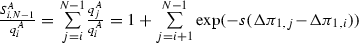
In Table 4 the fixation probabilities and time are indicated in the limit of large s. Moreover, the sign of the conditions can change with N for a given game, so the classification is N-dependent. As observed for large populations in the case of mutual invasion (scenario 2), the equilibrium frequency—represented for finite N by the i that minimizes \(|\Delta \pi _i|\)—is closer to fixation for the stronger invading strategy (A/B if \(\Delta \pi _1+\Delta \pi _{N-1}\gtrless 0\)) and this translates into guaranteed fixation for the strategy, though the required time exponentially diverges with the intensity of selection. Note that, by the linearity of the payoff differences \(\Delta \pi _i\) w.r.t. i, the quantity \(\Delta \pi _1+\Delta \pi _{N-1}\) is sign equivalent to the sum of \(\Delta \pi _i\) over all transient states (\(i=1,\ldots ,N-1\)) of the Markov chain. Stronger invasion thus also means that the strategy better performs, on average, over the possible compositions of the population.
We now address the case of extreme selection, in which the fittest strategy certainly reproduces in the Moran process and is certainly imitated in the pairwise comparison (technically it is the case with s at \(\infty \)). The transition probabilities become
0 otherwise, \(i=1,\ldots ,N-1\), so that it is impossible to step from i to \(i-1\) if \(\pi _{A,i}>\pi _{B,i}\) and to \(i+1\) if \(\pi _{A,i}<\pi _{B,i}\).
Consequently, the game classification results as in Table 5, where scenario 2 is indeed the coexistence scenario forbidden for finite populations and finite intensity of selection. This is not in contrast with Theorem 2, as the fixation probabilities are computed in Eqs. (10) and (14) assuming nonzero transition probabilities (Taylor et al. 2004). Increasing the selection intensity in scenario 2, some of the probability ratios in Eqs. (10) and (14) diverge and some others vanish, while their product behaves in accordance to Tables 3 and 4. For extreme selection, the products in Eqs. (10) and (14) are undefined and the Markov chain cannot step from state 1 to 0 and from state \(N-1\) to N, so that both fixation probabilities are zero (the fixation time is then undefined, because averaged by definition on the dynamics leading to fixation; similarly, the fixation time is undefined in scenario 3).
Finally, we derive the large-population-extreme selection limit of the two considered stochastic processes. From Eqs. (19) and (20), it immediately follows that when s is at \(\infty \), the deterministic limit becomes

\(\dot{x}=0\) otherwise. The corresponding evolutionary dynamics in scenarios (1A, 2, and 3) in Table 5 is pictured in Fig. 2. In both processes, the evolutionary rate \(\dot{x}\) vanishes while approaching the stable pure equilibria (filled dots at \(x=0\) and at \(x=1\) in Fig. 2), i.e., evolution slows down while reaching fixation. Indeed, the disappearing strategy has less and less chances to be selected for death in the Moran process and as focal in the pairwise comparison. In contrast, \(\dot{x}\) is discontinuous at the internal equilibrium \(x^*\) (see (21)), where it jumps from positive to negative values. The convergence/departure to/from stable/unstable internal equilibria thus occur at nonvanishing speed. Invasion, i.e., the departure from unstable pure equilibria, also occurs at nonzero speed in the Moran process (top panels), as the death of the resident strategist is guaranteed, whereas invasion gradually develops in the pairwise comparison (bottom panels) because limited by the selection of the invading strategist as role.

2.5 The (N, s)-Trade-off
The analysis in the two previous sections (summarized in Theorems 4 and 5 and Tables 3 and 4) shows that when either the population is sufficiently large or selection is sufficiently strong, only the competition scenarios 1–3, out of the 7 scenarios in Table 1, are possible in the Moran and pairwise comparison processes allowing any intensity of selection. How large N and s should be is however game-dependent. To estimate the (N, s) combinations for which the fraction of games showing scenarios 4–7 drops under a prescribed threshold, we have analyzed \(10^5\) randomly extracted games [independently uniformly distributed payoffs in [0, 1], as in Antal and Scheuring (2006) and Han et al. (2012)] for (N, s) ranging from \(N=4\) and \(s=10^{-2}\) up to \(N=10^5\) and \(s=10^4\) (logarithmically spaced, \(41 \times 61\) values). Recall that \(N\ge 3\) is required to independently discuss the invasion of strategies A and B, whereas \(N>3\) assures that fixation is fast in scenario 3 for sufficiently strong selection (see the proof of Theorem 5 in “Appendix” for more details).
The result is shown in Fig. 3, left and right panels for the Moran and pairwise comparison processes, respectively, where the gray-scale represents the fraction of games resulting in scenarios 4–7 for each considered pair (N, s) (from black, fraction \(=1\), to white, fraction \(=0\)). The fraction similarly vanishes in the main panels with both N and s and drops under \(10^{-3}\) in the considered (N, s) ranges. The fractions of the four scenarios are separately plotted in the minor panels (4–7) and interestingly show a few facts. While scenarios 4 (“invasion and slow fixation of one strategy”) is possible in small populations subject to weak selection and gradually disappear for increasing N and s, scenarios 5–7 persist to larger N and s (scenarios 5 and 7 in particular). And while 6 and 7 (“mutual invasion and slow fixation of both strategies” and “no invasion and fast fixation of one strategy”), perhaps the two most surprising, are most significant under weak selection (and intermediate population size), scenario 5 (“mutual invasion and fast fixation of one strategy”) requires an interchangeable mix of population size and selection. Moreover, while performing the analysis, we have checked that all the 7 scenarios (actually 12 scenarios counting symmetries) in Table 1 do occur generically (i.e., with non vanishing fraction for sufficiently small (N, s)), and that Conjectures 1 and 2 are never violated.

Fraction of the competition scenarios 4–7 in Table 1 in \(10^5\) random games (independently uniformly distributed payoffs a, b, c, d in [0, 1]), each analyzed on a grid of (logarithmically spaced) \(41\times 61\) pairs (N, s). Left/right: Moran/PWC process. Panels 4–7 separately refer to scenarios 4–7. The contour-lines in each panel correspond to fractions \(10^{-1}\), \(10^{-2}\), and \(10^{-3}\)
The figure does not show how the fractions of scenarios 4–7 is distributed over scenarios 1–3 while increasing N and s. When N is increased at constant s, this is known for the Moran process with linear fitness (Taylor et al. 2004; Antal and Scheuring 2006) and results are similar for the two processes here considered. When s is increased at constant N, the invasion scenario [that is N-dependent, recall the payoff differences \(\Delta \pi _1\) and \(\Delta \pi _{N-1}\) in Eqs. (9) and (13)] does not change, so that scenarios 4A and 4B turn into 1A and 1B, scenarios 5A and 5B turn into 2A and 2B, scenario 6 becomes 2A or 2B depending on the sign of \(\Delta \pi _1+\Delta \pi _{N-1}\) (that is also N-dependent), while scenarios 7A and 7B turn into 3.
Figure 3 shows that, while \(s=10^4\) is sufficient to rule out scenarios 4–7, the same cannot be said for \(N=10^5\), as a significant fraction of games end up in scenarios 5 and 7 for large N and mild selection. Some games require a larger population to adhere to the classification in Table 3. In particular, games characterized by small \(|b-d|\) or \(|a-c|\) (recall that our classification only considers generic games, i.e., games for which none of the classification criteria is undetermined; indeed none of the \(10^5\) extracted games have \(b=d\) or \(a=c\)). For example, if \(b-d=\varepsilon >0\) and \(c>d\), then \(\Delta \pi _1\) is positive for sufficiently large N (recall that \(\lim _{N\rightarrow \infty }\Delta \pi _1=b-d\)), but it is negative for \(N<(c-d)/\varepsilon +1\) [easy to check from Eq. (9)], a threshold that can be arbitrarily large for sufficiently small \(\varepsilon \). Vice versa, if \(b-d=-\varepsilon \) and \(c<d\), then \(\Delta \pi _1\) is negative for sufficiently large N, though positive for \(N<(d-c)/\varepsilon +1\). And similarly for the effect of a small \(|a-c|\) on \(\Delta \pi _{N-1}\) [see Eq. (13)].

Change of competition scenario for increasing N for two critical games with small \(|b-d|\) played under weak (bottom) and strong (top) selection
Figure 4 shows how the competition scenario changes for increasing N in the two above critical cases, the first (left) with \(b-d=\varepsilon \), \(c>d\), \(a=0\) (B dominance/coexistence at low/high N), the second (right) with \(b-d=-\varepsilon \), \(c=0\), \(a>0\) (A dominance/mutual exclusion at low/high N). Note that even when selection is very strong (top part of the figure), scenarios 5 and 7 appear while increasing N before the asymptotic scenario for large N shows up. This means that there are critical games that, when played in intermediate sized populations, require arbitrarily strong selection to show the asymptotic scenario for large s. Indeed, regardless of how strong selection is, fixing N in the range in which the resulting scenario is 5/7 in Fig. 4, left/right, then a higher intensity of selection is required to reach the asymptotic scenario for large s. In other words, even if we basically see white in the top part of all panels in Fig. 3, scenarios 5 and 7 might occur for any s, though the fraction of these critical games vanishes with both s and N.
Computationally, determining the fixation time for large N is the most expensive operation and the analysis of a single game for a single pair (N, s) takes memory and time proportionally to N. In particular, determining the fixation time is more demanding when fixation is fast, because all elements in the sum defining \(t_{\text {fix}}^A\) or \(t_{\text {fix}}^B\) [see Eqs. (12) and (15)] must be computed to check the sum to be smaller than the fixation time in the neutral game. To save computational time, we have used the following heuristic: for each considered value of s, if the competition scenario for \(N>10^3\) is 1 or 3 (i.e., a fast asymptotic scenario for large N) and fixation results fast for 5 consecutive values of N (and same s) in our grid, we then assume fast fixation for larger N and avoid the computation of the fixation time, provided the directions of the invasion and fixation arrows do not change. So doing, the most demanding games are of asymptotic scenario 2 for large N (“mutual invasion and slow fixation of one strategy”), in which however fixation remains fast up to large N (Fig. 4, left). Vice versa, games in which fixation is asymptotically fast for large N (asymptotic scenarios 1 or 3, see, e.g., Fig. 4, right) are less demanding, because either fixation becomes fast at intermediate N and our heuristic applies, or fixation remains slow up to large N.
For example, the most demanding game in Fig. 3 turned out to be \(a=0.4857\), \(b=0.1746\), \(c=0.6908\), \(d=0.1745\), indeed of the type with \(b-d=\varepsilon =10^{-4}\) and \(c>d\) (Fig. 4, left). To be analyzed over all \(41 \times 61\) considered (N, s)-pairs, it required 47602 s. of CPU time, with worst case of 361 s. for \((N,s)=(10^5,10^{-2})\) (using an optimized compiled MATLAB script on a dedicated core of a CPU Intel Xenon E5-2650@2GHz under linux Ubuntu 14.04). On average, each game required (over all (N, s)-pairs) 645 s. of CPU time, i.e., a total computational time of about 2 years of CPU time for producing Fig. 3 (about one month of physical time on our 32-core machine).
3 Discussion
We have considered the simplest setting of a 2-player-2-strategy symmetric game in finite populations, equipped with the two most common microscopic models of strategy spreading allowing any intensity of selection—the frequency-dependent Moran process and the pairwise comparison process both based on the exponential fitness (see (Traulsen et al. 2006, 2007, 2008), respectively). In line with the literature on evolutionary games in finite populations (Nowak et al. 2004; Taylor et al. 2004, 2006; Nowak 2006; Antal and Scheuring 2006), the stochastic evolution of a strategy is characterized by its chances of invasion—whether initial spreading from a single strategist is more or less likely than extinction—by its chances of fixation—the probability to take over the whole population starting from a single strategist—and by the expected fixation time—the average number of transitions to fixate. Specifically, fixation is defined using the neutral game with equal expected payoffs for both strategies as benchmark. A strategy is shortly said to fixate if the fixation probability is higher than in the neutral game and fixation is said to be fast or slow if the average fixation time is smaller or larger compared to the neutral game.
Our main contribution is showing that when selection is sufficiently strong, out of the seven invasion and fixation scenarios that are generically possible (reported in Table 1), only three can occur and are the same three that are possible in large populations: (1) invasion and fast fixation of one strategy; (2) mutual invasion and slow fixation of one strategy; (3) no invasion and no (fast) fixation. This somehow unifies evolutionary game dynamics in finite and infinite populations, though the same game (same payoff matrix) can still fall into different classes (among 1–3) if played within a large group with mild selection or within a small group with strong selection. This is essentially due to the fact that the invasion scenario can change for increasing population size, while it is independent of selection intensity. Hence, for a given game, the limiting classes for large population and extreme selection can differ, though they coincide if selection intensity is large enough in the first limit and population size in the second. The result is therefore independent of the order in which the two limits are taken (compare Tables 3 and 4 and recall that the conditions in Table 4 coincide with those in Table 3 for large N), contrary to what found for the opposite extreme of weak selection (Sample and Allen 2016).
Another interesting contribution comes from the limit to extreme selection, in which the coexistence scenario 2 becomes mutual invasion with no chances for fixation, a case not possible (by Theorem 2) for finite intensity of selection that better corresponds to the deterministic case of coexistence. Indeed, under mutual invasion and strong but finite selection, fixation is eventually guaranteed for the stronger invading strategy—that is also the more frequent strategy at coexistence and the one that better performs, on average, over the possible compositions of the population—while it is unreachable for the other strategy. The fixation time, however, exponentially diverges with the intensity of selection (see Table 4). The two strategies coexist for a long time by fluctuating around an intermediate frequency—at which the expected payoffs essentially balance—before the better performing strategy takes over the whole population. Discussing fixation for coexistence games in the strong selection limit has hence limited practical interest, though theoretically it is part of the game classification. As long as the intensity of selection is finite, coexistence games show an apparent contradiction, as fixation might seem more likely while moving at random in the neutral game than while competing against an invading strategy. When selection is extreme, this becomes indeed the case, as the fixation probabilities for both strategies drop to zero (see Table 5).
We give three other (minor) contributions. First, we have shown that the game classification in Table 1, originally proposed and shown for the Moran process with linear fitness (Taylor et al. 2004; Antal and Scheuring 2006), works as well for the Moran and pairwise comparison processes allowing any intensity of selection. To keep the classification compact, we have focused only on generic games, i.e., games for which none of the classification criteria is undetermined (because the equal sign holds true instead of the inequality). Non-generic cases are exceptional in the set of all possible games, but not necessarily of little interest, e.g., the theoretically important neutral game.
Second, we have shown how the classification simplifies to the three competition scenarios 1–3 in large populations, again analogously to what shown for the Moran process with linear fitness (Taylor et al. 2004; Antal and Scheuring 2006).
Third, in the extreme selection limit, we have derived the large population deterministic limit, showing that for both the Moran and pairwise comparison processes the replicator dynamics become discontinuous at intermediate equilibria.
We have also numerically estimated the intensity of selection s and the population size N required to rule out the competition scenarios 4–7, by means of a Monte Carlo analysis of \(10^5\) games (payoff matrices) each on a grid of \(41 \times 61\) (N, s) pairs. Scaling the game payoffs in [0, 1], it turned out that \(s=10^4\) makes the fraction of games in scenarios 4–7 drop below \(10^-3\) for all N, whereas \(N=10^5\) leaves a small but significant fraction of such games for weak and mild selection. More specifically, while scenario 4 (“mutual invasion and fast fixation of one strategy”) is gradually replaced by its fast counterpart for increasing s and N, scenarios 5 and 7 (“mutual invasion and fast fixation of one strategy” and “no invasion and fast fixation of one strategy”) are possible under arbitrarily strong selection in arbitrarily large populations, whereas the weird scenario 6 (in which both strategies invade and fixate) is most significant under weak selection and intermediate population size.
The analysis for populations larger than \(N=10^5\) is computationally too expensive and is not presented. Our focus is on strong selection, and our analysis shows that in small-medium groups (10–1000 individuals) selection needs to be very strong (\(s\approx 10^4\)) to rule out scenarios 5 and 7. Thus, though theoretically not possible for sufficiently strong and extreme selection, these scenarios do play a role in many practical applications.
Although derived for a special pair of processes of strategy spreading—the Moran and pairwise comparison processes based on the exponential fitness—that share the same fixation probabilities (Wu et al. 2015), our results can be generalized to other functional forms for the fitness in the Moran process and for the imitation probability in the pairwise comparison. Theorems 1–3—on which the classification in Table 1 is essentially based—and Theorem 4—addressing the large population limit—can be generalized to any increasing fitness function and to any imitation probability that increases with the expected payoff gain. The proofs would essentially retrace those in Taylor et al. (2004) and in Antal and Scheuring (2006) for the Moran process with linear fitness. The only relevant change would be the condition in Table 3 that discriminates who is fixing in a coexistence game in large populations. With the exponential fitness, this condition turns out to be very simple and interpretable—the more frequent strategy at coexistence—whereas a more complex expression was, for example, obtained for the linear fitness (Antal and Scheuring 2006). In general, products of fitness ratios would be involved for a generically increasing fitness.
To generalize Theorem 5, we need an extra assumption. Indeed, to discuss any intensity of selection, we need the better performing strategy to reproduce or be copied with a probability that increases with the strength of selection, and that reaches one when selection is extreme. This translates into the following limiting property for the ratio of the transition probabilities from state i, \(\lim \limits _{s\rightarrow \infty }T^-_i/T^+_i=0\) if \(\Delta \pi _i> 0\) (and consequently the limit diverges to \(\infty \) if \(\Delta \pi _i< 0\)). The property requires, for the Moran process, a fitness function that grows faster than any polynomial, then making the exponential function the most natural choice, though mathematically there are other options. What would change by considering other options is again the condition discriminating who is fixing in a coexistence game. With the exponential fitness, this condition in Table 4 is fully analogous to that in Table 3, whereas more complex and less interpretable expressions would be obtained with other functional forms. It is therefore possible that the same game, played with the same population size and selection intensity, is differently classified by two different fitness formulations in the Moran process or two different imitation probabilities in the pairwise comparison. How the classification changes for increasing N and s—our main contribution—remains however a general result.
Strong and extreme selection were previously considered by other authors, though the analysis of the game classification remained unexplored even in the simple settings of 2-player-2-strategy symmetric games. Altrock and Traulsen (2009) proposed a modified Moran process in which selection acts on both reproduction and death, thus obtaining, in the limit of extreme selection, a deterministic evolutionary dynamics in finite populations. With respect to their results, we have shown that a fully deterministic dynamics in finite populations is not necessary for matching the competition scenarios 1–3 in finite and infinite populations. Our two semi-deterministic processes (Moran and pairwise comparison) are enough.
Antal et al. (2009) and Wu et al. (2013) also considered the pairwise comparison process under any intensity of selection, both focusing on the relative abundance of two (or more) strategies in terms of the stationary distribution of the lumped Markov chain between the pure states, with transition triggered by mutations. Surprisingly, while the ranking of strategy abundances is not affected by the functional form used for the imitation probability in 2-player-2-strategy games (Antal et al. 2009), differences are often observed for games with either more strategies or more players (Wu et al. 2013). These results are however not directly comparable with the game classification here discussed, where mutations are not considered and coexistence games prevent the discussion of the lumped transitions between pure states. Our intuition is that our main result—the invasion and fixation scenarios that are possible for strong selection are the same observed in large populations—remains valid also for games with more players and/or strategies, independently of the specific choice of the functional forms of the mechanism of strategy spreading. Checking this intuition is however left for further research.
References
Altrock PM, Traulsen A (2009) Deterministic evolutionary game dynamics in finite populations. Phys Rev E 80(1):011909
Antal T, Scheuring I (2006) Fixation of strategies for an evolutionary game in finite populations. Bull Math Biol 68(8):1923–1944
Antal T, Nowak MA, Traulsen A (2009) Strategy abundance in games for arbitrary mutation rates. J Theor Biol 257:340–344
Ashcroft P, Traulsen A, Galla T (2015) When the mean is not enough: calculating fixation time distributions in birth–death processes. Phys Rev E 92:042154
Blume LE (1993) The statistical mechanics of strategic interaction. Games Econ Behav 5(3):387–424
Fudenberg D, Nowak MA, Taylor C, Imhof LA (2006) Evolutionary game dynamics in finite populations with strong selection and weak mutation. Theor Popul Biol 70(3):352–363
Han TA, Traulsen A, Gokhale CS (2012) On equilibrium properties of evolutionary multi-player games with random payoff matrices. Theor Popul Biol 81:264–272
Hofbauer J, Sigmund K (1998) Evolutionary games and population dynamics. Cambridge University Press, Cambridge
Maynard Smith J (1982) Evolution and the theory of games. Cambridge University Press, Cambridge
Maynard Smith J, Price J (1973) The logic of animal conflicts. Nature 246:15–18
Nowak MA (2006) Evolutionary dynamics. Harvard University Press, Cambridge
Nowak MA, Sasaki A, Taylor C, Fudenberg D (2004) Emergence of cooperation and evolutionary stability in finite populations. Nature 428:646–650
Sample C, Allen B (2016) The limits of weak selection and large population size in evolutionary game theory. ArXiv:1610.07081 [q-bio.PE]
Szabó G, Tőke C (1998) Evolutionary prisoner’s dilemma game on a square lattice. Phys Rev E 58:69–73
Taylor PJ, Jonker L (1978) Evolutionarily stable strategies and game dynamics. Math Biosci 40:145–156
Taylor C, Fudenberg D, Sasaki A, Nowak MA (2004) Evolutionary game dynamics in finite populations. Bull Math Biol 66(6):1621–1644
Taylor C, Iwasab Y, Nowak MA (2006) A symmetry of fixation times in evolutionary dynamics. J Theor Biol 243:245–251
Traulsen A, Hauert C (2009) Stochastic evolutionary game dynamics. Reviews of nonlinear dynamics and complexity, Vol II. Wiley-VHC, New York, New York, pp 25–61
Traulsen A, Claussen JC, Hauert C (2005) Coevolutionary dynamics: from finite to infinite populations. Physical Rev Lett 95(23):238701
Traulsen A, Nowak MA, Pacheco JM (2006) Stochastic dynamics of invasion and fixation. Phys Rev E 74:011909
Traulsen A, Pacheco JM, Nowak MA (2007) Pairwise comparison and selection temperature in evolutionary game dynamics. J Theor Biol 246(3):522–529
Traulsen A, Shoresh N, Nowak MA (2008) Analytical results for individual and group selection of any intensity. Bull Math Biol 70(5):1410–1424
Wu B, Altrock PM, Wang L, Traulsen A (2010) Universality of weak selection. Phys Rev E 82:046106
Wu B, García J, Hauert C, Traulsen A (2013) Extrapolating weak selection in evolutionary games. PLoS Comput Biol 9(12):e1003381
Wu B, Bauer B, Galla T, Traulsen A (2015) Fitness-based models and pairwise comparison models of evolutionary games are typically different—even in unstructured populations. New J Phys 17:023043
Acknowledgements
We like to thank Arne Traulsen (Max-Planck-Institute for Evolutionary Biology, Plön, Germany) for useful comments on an early draft of this manuscript, and we also acknowledge the contribution of one anonymous reviewer. The work was supported by the Italian Ministry for Education, University, and Research (under contract FIRB RBFR08TIA4).
Author information
Authors and Affiliations
Corresponding author
Additional information
This work was supported by the Italian Ministry for Education, University, and Research (under contract FIRB RBFR08TIA4).
Appendix: Proofs of Theorems 1–5
Appendix: Proofs of Theorems 1–5
Before proving Theorems 1–5, we recall, for the reader’s convenience, a few definitions used throughout the proofs.
-
The difference between the expected payoffs for strategies A and B at state i
$$\begin{aligned} \Delta \pi _i=\pi _{A,i}-\pi _{B,i}= \frac{\Delta \pi _1(N-1-i)+\Delta \pi _{N-1}(i-1)}{N-2}, \end{aligned}$$(24a)\(i=1,\ldots ,N-1\), here rewritten from Eq. (8) in terms of
$$\begin{aligned} \Delta \pi _1=b-\displaystyle \frac{\displaystyle c+d(N-2)}{\displaystyle N-1} \quad \text {and}\quad \Delta \pi _{N-1}=\displaystyle \frac{\displaystyle a(N-2)+b}{\displaystyle N-1}-c \end{aligned}$$(24b)ruling strategy invasion.
-
The sum of all, the first j, and the last l expected payoff differences
 (25a)
(25a) (25b)
(25b) (25c)
(25c) -
The fixation probabilities \(P_{\text {fix}}^A=1/S^A_{0,N-1}\) and \(P_{\text {fix}}^B=1/S^B_{0,N-1}\) for strategies A and B, where
 (26a)
(26a) (26b)
(26b)are rewritten from Eqs. (10) and (14) in terms of the sums in (25b,c).
-
The two equivalent formulations for the fixation time
 (27a)
(27a) (27b)
(27b)where \(q^A_0=q^B_0=1\) and indexes i, j and k, l count the number of A and B-strategists, respectively (see Eqs. (12) and (15) and take the transition probabilities (2, 3), and (4, 5) and property (7) into account).


Moreover, we graph in Fig. 5 the quantities in (24) and (25) in six cases with \(N=10\) representative of the competition scenarios in Table 1. The figure will support the statements in the proofs. Throughout this “Appendix” we assume a positive intensity of selection (\(s>0\)).

Profiles of the payoff differences \(\Delta \pi _i\) (linear w.r.t. i, see Eq. (24a), top panel) and of the partial sums \(\Delta \pi _{1,j}\) and \(\Delta \pi _{N-l,N-1}\) (quadratic with j and l, see Eqs. (25b, c), bottom panel) in the competition scenarios in Table 1 (\(N=10\)). Recall that, by the linearity of \(\Delta \pi _i\), the sum of all payoff differences \(\Delta \pi _{1,N-1}\) [Eq. (25a)] is sign equivalent to the sum \(\Delta \pi _1+\Delta \pi _{N-1}\) of the first and last differences
Theorem 1
If A/B invades and B/A does not, then A/B fixates and B/A does not.
Proof
We need to prove that if \(\Delta \pi _1>0\) and \(\Delta \pi _{N-1}>0\) (A invades and B does not), then \(P_{\text {fix}}^A>1/N\) and \(P_{\text {fix}}^B<1/N\) (A fixates and B does not). The other case (\(\Delta \pi _1<0\) and \(\Delta \pi _{N-1}<0\)) follows by the interchange of A and B.
\(\Delta \pi _1>0\) and \(\Delta \pi _{N-1}>0\) imply \(\Delta \pi _{1,j}>0\) and \(\Delta \pi _{N-l,N-1}>0\) for all \(j,l=1,\ldots ,N-1\) (see gray and white dots in Fig. 5, 1A, respectively). Consequently, all elements in the sum in (26a) are smaller than one and all elements in the sum in (26b) are larger than one. We hence have \(P_{\text {fix}}^A=1/S^A_{0,N-1}>1/N\) and \(P_{\text {fix}}^B=1/S^B_{0,N-1}<1/N\).
\(\square \)
Theorem 2
If neither A nor B fixate, then neither A nor B invade.
Proof
We prove the theorem by contradiction, i.e., we show that if at least A or B invades, then at least A or B fixates. If only one strategy invades, the latter statement is true by Theorem 1. It hence remains to be proved that when A and B both invade (\(\Delta \pi _1>0\) and \(\Delta \pi _{N-1}<0\)), then at least A or B fixates (\(P_{\text {fix}}^A>1/N\) or \(P_{\text {fix}}^B>1/N\)).
Assume then \(\Delta \pi _1>0\) and \(\Delta \pi _{N-1}<0\). If \(\Delta \pi _1+\Delta \pi _{N-1}>0\), i.e., \(\Delta \pi _{1,N-1}>0\), then \(\Delta \pi _{1,j}>0\) for all \(j=1,\ldots ,N-1\) (see gray dots in Fig. 5, 2A), so that all elements in the sum in (26a) are smaller than one and \(P_{\text {fix}}^A=1/S^A_{0,N-1}>1/N\) (A fixates). Vice versa, if \(\Delta \pi _1+\Delta \pi _{N-1}<0\), i.e., \(\Delta \pi _{1,N-1}<0\), then \(\Delta \pi _{N-l,N-1}<0\) for all \(l=1,\ldots ,N-1\) (see white dots in Fig. 5, 2B), so that all elements in the sum in (26b) are smaller than one and \(P_{\text {fix}}^B=1/S^B_{0,N-1}>1/N\) (B fixates). \(\square \)
Theorem 3
If A and B both fixate, then A and B both invade.
Proof
We prove the theorem by contradiction, i.e., we show that if at least A or B does not invade, then at least A or B does not fixate. If only one strategy invades, the latter statement is true by Theorem 1. It hence remains to be proved that when neither A nor B invade (\(\Delta \pi _1<0\) and \(\Delta \pi _{N-1}>0\)), then at least A or B does not fixate (\(P_{\text {fix}}^A<1/N\) or \(P_{\text {fix}}^B<1/N\)).
Assume then \(\Delta \pi _1<0\) and \(\Delta \pi _{N-1}>0\). If \(\Delta \pi _1+\Delta \pi _{N-1}>0\), i.e., \(\Delta \pi _{1,N-1}>0\), then \(\Delta \pi _{N-l,N-1}>0\) for all \(l=1,\ldots ,N-1\) (see white dots in Fig. 5, 7A), so that all elements in the sum in (26b) are larger than one and \(P_{\text {fix}}^B=1/S^B_{0,N-1}<1/N\) (B does not fixate). Vice versa, if \(\Delta \pi _1+\Delta \pi _{N-1}<0\), i.e., \(\Delta \pi _{1,N-1}<0\), then \(\Delta \pi _{1,j}<0\) for all \(j=1,\ldots ,N-1\) (see gray dots in Fig. 5, 7B), so that all elements in the sum in (26a) are larger than one and \(P_{\text {fix}}^A=1/S^A_{0,N-1}<1/N\) (A does not fixate). \(\square \)
Theorem 4 addresses the limit \(N\rightarrow \infty \). For this, we consider the frequency \(x=i/N\) (or \(x=j/N\)) of A-strategists and the frequency \(1-x=k/N\) (or \(1-x=l/N\)) of B-strategists, and we rewrite the payoff differences in (24) and the sums in (25) for large N as
and


We also recall the limits for large N of the transition probabilities (2, 3) and (4, 5), i.e.,
and
and the equilibrium frequency (21)
To study the fixation time for large N [following Antal and Scheuring (2006)], we evaluate the sums in (27a) around the frequencies x at which the corresponding elements of the sum diverge with N. Only these dominant elements can give contributions that are more than linear with N and therefore make fixation slow (recall that the fixation time is quadratic with N in the neutral game, \(N(N-1)\) and \(2N(N-1)\) in the Moran and pairwise comparison cases, respectively).
Before proving Theorem 4, we show the following
Lemma 1
Proof
For large N and any finite j, we have \(\Delta \pi _{1,j}\approx j(b-d)\) [from (25b)] and  [from (25a)]. Under \(b-d+a-c>0\), the sum \(S^A_{0,N-1}\) is then dominated by the first elements and behaves as a geometric series (convergent if \(b-d>0\); divergent if \(b-d<0\)). Otherwise, if \(b-d+a-c<0\), the last elements of \(S^A_{0,N-1}\) exponentially diverge with N.
The results on the sum \(S^B_{0,N-1}\) similarly follow. For large N and any finite l, we have \(\Delta \pi _{N-l,N-1}\approx l(a-c)\) [from (25c)] and  (again from (25a)). Under \(b-d+a-c<0\), the sum is dominated by the first elements and behaves as a geometric series (convergent if \(a-c<0\); divergent if \(a-c>0\)). Otherwise, if \(b-d+a-c<0\), the last elements of \(S^B_{0,N-1}\) exponentially diverge with N. \(\square \)
We also recall that the game classification in Table 3 considers only generic games, i.e., those for which no condition is undetermined.
Theorem 4
For each generic game (a, b, c, d) there is a population size \(N^{\infty }\) such that the game classification is as in Table 3 for any \(N>N^{\infty }\).
Proof
Separately for each of the five competition scenarios in Table 3, we prove that the corresponding conditions imply the scenario for sufficiently large N. The theorem follows by the fact that the union of the five sets of (mutually exclusive) conditions covers all generic games.
- 1A :
-
If \(b-d>0\) and \(a-c>0\) (A invades and B does not), then, by Lemma 1, \(P_{\text {fix}}^A\) and \(P_{\text {fix}}^B\) behave for large N as in Table 3. To estimate the fixation time, we use (27a, left) in which we note that \(S^A_{0,i-1}\) increases with i from 1 at \(i=1\) to \(S^A_{0,N-1}\) (finite by Lemma 1) at \(i=N\) and that
 (32)
(32)decreases with i from \(S^A_{0,N-1}\) at \(i=0\) to 1 at \(i=N-1\) (also note that \(\Delta \pi _{1,j}-\Delta \pi _{1,i}>0\) in (32) since \(j>i\), see gray dots in Fig. 5, 1A). All terms in (27a, left) but the transition probability \(T^+_i\) are therefore positive and bounded for \(x\in (0,1)\), whereas \(T^+_i\) (at denominator in \(t_{\text {fix}}\)) vanishes at \(x=0\) and \(x=1\) [see Eq. (30a)], where it behaves as
$$\begin{aligned} T^+(x)|_{x=0}\approx \left\{ \begin{array}{ll} \frac{x}{\exp (-s(b-d))} &{} \text { Moran}\\ \frac{x}{1+\exp (-s(b-d))} &{} \text { PWC} \end{array}\right. \end{aligned}$$(33a)and
$$\begin{aligned} T^+(x)|_{x=1}\approx \left\{ \begin{array}{ll} 1-x &{} \text { Moran} \\ \frac{1-x}{1+\exp (-s(a-c))} &{} \text { PWC} \end{array}\right. \end{aligned}$$(33b)The two dominant contributions to \(t_{\text {fix}}\) hence come from the elements in (27a, left) around \(x=0\) and \(x=1\). Using the asymptotic of the Harmonic series, both contributions are proportional to
 (34)
(34) - 1B :
-
If \(b-d<0\) and \(a-c<0\) (B invades and A does not), the analysis is symmetric to case 1A (by the interchange of A and B). Specifically, by Lemma 1, \(P_{\text {fix}}^A\) and \(P_{\text {fix}}^B\) behave for large N as in Table 3. To estimate the fixation time, we use (27a, right) in which we note that \(S^B_{0,k-1}\) increases with k from 1 at \(k=1\) to \(S^B_{0,N-1}\) (finite by Lemma 1) at \(k=N\) and that
 (35)
(35)decreases with k from \(S^B_{0,N-1}\) at \(k=0\) to 1 at \(k=N-1\) (also note that \(\Delta \pi _{N-l,N-1}-\Delta \pi _{N-k,N-1}<0\) in (35) since \(l>k\), see white dots in Fig. 5, 1B). All terms in (27a, right) but the transition probability \(T^-_{N-k}\) are therefore positive and bounded for \(x\in (0,1)\), whereas \(T^-_{N-k}\) (at denominator in \(t_{\text {fix}}\)) behaves for large N as \(T^-_{N-k}|_{k=(1-x)N}=T^-_i|_{i=xN}\) and vanishes at \(x=0\) and \(x=1\) [see Eq. (30b)], where it behaves as
$$\begin{aligned} T^-(x)|_{x=0}\approx \left\{ \begin{array}{ll} x &{} \text { Moran}\\ \frac{x}{1+\exp (s(b-d))} &{} \text { PWC} \end{array}\right. \end{aligned}$$(36a)and
$$\begin{aligned} T^-(x)|_{x=1}\approx \left\{ \begin{array}{ll} \frac{1-x}{\exp (s(a-c))} &{} \text { Moran}\\ \frac{1-x}{1+\exp (s(a-c))} &{} \text { PWC} \end{array}\right. \end{aligned}$$(36b)The two dominant contributions to \(t_{\text {fix}}\) hence come from the elements in (27a, right) around \(x=0\) and \(x=1\). As in case 1A, both contributions are proportional to \(N\log N\).
- 2A :
-
If \(b-d>0\) and \(a-c<0\) with \(b-d+a-c>0\) (both A and B invade and selection favors A), then, by Lemma 1, \(P_{\text {fix}}^A\) and \(P_{\text {fix}}^B\) behave for large N as in case 1A. The fixation time however diverges exponentially due to the contribution of (32) in (27a, left). In fact, while \(S^A_{0,i-1}\) and the transition probability \(T^+_i\) behave as in case 1A, the difference \(\Delta \pi _{1,j}-\Delta \pi _{1,i}\) in (32) is negative for several i, j. The most negative value is attained for \(i=i^*\), where \(\Delta \pi _{1,i^*}\) is the largest of \(\Delta \pi _{1,j}\) (see gray dots in Fig. 5, 2A; \(i^*\) corresponds to the last positive \(\Delta \pi _i\), see black dots), and for \(j=N-1\). For large N, \(i^*\approx \lfloor x^*N\rfloor \), where \(x^*\in (0,1)\) from (31, left) maximizes the downward parabola \(\Delta \pi _{1,j}/N\) in (29b) (\(\lfloor i\rfloor \) taking the integer part of i), so that the most negative difference \(\Delta \pi _{1,N-1}-\Delta \pi _{1,i^*}\) behaves as \(\frac{\scriptstyle N}{\scriptstyle 2}{} \big ((b-d+a-c)-(b-d)^2/(b-d-a+c)\big )\) (obtained from (29b) at \(x=1\) and at \(x=x^*\)). The linear N-dependence of the latter expression makes (32) exponentially diverging with N.
- 2B :
-
If \(b-d>0\) and \(a-c<0\) with \(b-d+a-c<0\) (both A and B invade and selection favors B), then, by Lemma 1, \(P_{\text {fix}}^A\) and \(P_{\text {fix}}^B\) behave for large N as in case 1B. The fixation time however diverges exponentially for large N due to the contribution of (35) in (27a, right). In fact, while \(S^B_{0,k-1}\) and the transition probability \(T^-_{N-k}\) behave as in case 1B, the difference \(\Delta \pi _{N-l,N-1}-\Delta \pi _{N-k,N-1}\) in (35) is positive for several k, l. The most positive value is attained for \(k=k^*\), where \(\Delta \pi _{N-k^*,N-1}\) is the most negative of \(\Delta \pi _{N-l,N-1}\) (see white dots in Fig. 5, 2B; \(k^*\) corresponds to the last negative \(\Delta \pi _{N-k}\), see black dots), and for \(l=N-1\). For large N, \(k^*\approx \lfloor (1-x^*)N\rfloor \), where \(1-x^*\in (0,1)\) from (31, right) minimizes the upward parabola \(\Delta \pi _{N-l,N-1}\) in (29c), so that the most positive difference \(\Delta \pi _{1,N-1}-\Delta \pi _{N-k^*,N-1}\) behaves as \(\frac{\scriptstyle N}{\scriptstyle 2}{} \big ((b-d+a-c)+(a-c)^2/(b-d-a+c)\big )\) (obtained from (29c) at \(1-x=1\) and at \(1-x=1-x^*\)). The linear N-dependence of the latter expression makes (35) exponentially diverging with N.
- 3:
-
If \(b-d<0\) and \(a-c>0\) (both A and B do not invade), then, by Lemma 1, \(P_{\text {fix}}^A\) and \(P_{\text {fix}}^B\) behave for large N as in Table 3. To estimate the fixation time, we use (27a, left). If \(i\le i^*\), where \(\Delta \pi _{1,i^*}\) is the most negative of \(\Delta \pi _{1,j}\) (see gray dots in Fig. 5, 3; \(i^*\) corresponds to the last negative \(\Delta \pi _i\), see black dots), we exploit \(q^A_i=(T^-_i/T^+_i)q^A_{i-1}\) and rewrite the element of the sum (27a, left) as
 (37)
(37)In (37), we note that \(\lim _{N\rightarrow \infty }S^A_{i,N-1}/S^A_{0,N-1}=1\), as the sums \(S^A_{i,N-1}\) and \(S^A_{0,N-1}\) are dominated for large N by the same element at \(j=i^*\), that
 (38)
(38)increases with i from 1 at \(i=1\) to \(1/(1-\exp (s(b-d)))\) at \(i=i^*\) (using \(\Delta \pi _{1,j}-\Delta \pi _{1,i-1}\approx -(i-1-j)(b-d)>0\) from (25b) for large N and noting that \(i^*\approx \lfloor x^*N\rfloor \) diverges with N, so the sum in (38) is a convergent geometric series), and that \(T^-_i\) at denominator behaves as in (30b). If \(i>i^*\), we directly use (27a, left) in which \(\lim _{N\rightarrow \infty }S^A_{0,i-1}/S^A_{0,N-1}=1\), as the sums \(S^A_{0,i-1}\) and \(S^A_{0,N-1}\) are those dominated by the element at \(j=i^*\), (32) decreases with i from \(1/(1-\exp (-s(a-c)))\) at \(i=i^*\) (using \(\Delta \pi _{1,j}-\Delta \pi _{1,i}\approx \Delta \pi _{N-(j-i),N-1}\approx (j-i)(a-c)>0\) from (25c) for large N and noting that \(N-1-i^*\approx \lfloor (1-x^*)N\rfloor \) diverges with N, so the sum in (32) is a convergent geometric series) to 1 at \(i=N-1\), and the transition probability \(T^+_i\) at denominator behaves as in (30a).
The dominant elements in (27a, left) are hence those around \(x=0\) for \(i\ge i^*\), where the transition probability \(T^-_i\) vanishes as in (36a), and those around \(x=1\) for \(i>i^*\), where the transition probability \(T^+_i\) vanishes as in (33b). As in case 1A, both contributions to \(t_{\text {fix}}\) are proportional to \(N\log N\).


\(\square \)
Theorem 5 addresses the limit \(s\rightarrow \infty \). For this, we take the limit for large s of the transition probabilities (2, 3) and (4, 5), obtaining

and

\(i=1,\ldots ,N-1\), and we show the following
Lemma 2
Proof
The lemma directly follows from the expressions of \(S^A_{0,N-1}\) and \(S^B_{0,N-1}\) in (26), by noting that the four cases, respectively, correspond to \(\Delta \pi _{1,j}>0\) for all \(j=1,\ldots ,N-1\), \(\Delta \pi _{1,j}<0\) for some j, \(\Delta \pi _{N-l,N-1}<0\) for all \(l=1,\ldots ,N-1\), and \(\Delta \pi _{N-l,N-1}>0\) for some l. \(\square \)
We also recall that the game classification in Table 4 considers only generic games, i.e., those for which no condition is undetermined.
Theorem 5
For each generic game (a, b, c, d) there is an intensity of selection \(s^{\infty }\) such that the game classification is as in Table 4 for any \(s>s^{\infty }\).
Proof
Separately for each of the five competition scenarios in Table 4, we prove that the corresponding conditions imply the scenario for sufficiently large s. The theorem follows by the fact that the union of the five sets of (mutually exclusive) conditions covers all generic games.
- 1A :
-
If \(\Delta \pi _1>0\) and \(\Delta \pi _{N-1}>0\) (A invades and B does not), then \(\Delta \pi _1+\Delta \pi _{N-1}>0\), so that by Lemma 2 \(P_{\text {fix}}^A\) and \(P_{\text {fix}}^B\) behave for large s as in Table 4. To estimate the fixation time, we use (27a, left) in which we note that \(\lim _{s\rightarrow \infty }S^A_{0,i-1}=\lim _{s\rightarrow \infty }S^A_{0,N-1}=1\), as all elements but the first (\(q^A_0=1\)) of both sums vanish as \(s\rightarrow \infty \), and that \(\lim _{s\rightarrow \infty }S^A_{i,N-1}/q^A_i=1\), as \(q^A_i\) is the dominant element in \(S^A_{i,N-1}\) for large s (\(\Delta \pi _{1,i}\) is the smallest of \(\Delta \pi _{1,j}\) for \(j=i,\ldots ,N-1\), see gray dots in Fig. 5, 1A). Using (39a), the fixation time is then given by
 (40)
(40)where the inequalities hold true for \(N\ge 3\) (Moran: all elements but the last in the right-most sum are \(<1\), the last being \(=1\); PWC: all elements in the right-most sum are \(<2\), being all \(\le N/(N-1)\) that is \(<2\) for \(N\ge 3\)).
- 1B :
-
If \(\Delta \pi _1<0\) and \(\Delta \pi _{N-1}<0\) (B invades and A does not), the analysis is symmetric to case 1A (by the interchange of A and B). Specifically, \(\Delta \pi _1+\Delta \pi _{N-1}<0\), so that by Lemma 2 \(P_{\text {fix}}^A\) and \(P_{\text {fix}}^B\) behave for large s as in Table 4. To estimate the fixation time, we use (27a, right), in which we note that \(\lim _{s\rightarrow \infty }S^B_{0,k-1}=\lim _{s\rightarrow \infty }S^B_{0,N-1}=1\), as all elements but the first (\(q^B_0=1\)) of both sums vanish as \(s\rightarrow \infty \), and that \(\lim _{s\rightarrow \infty }S^B_{k,N-1}/q^B_k=1\), as \(q^B_k\) is the dominant element in \(S^B_{k,N-1}\) for large s (\(\Delta \pi _{N-k,N-1}\) is the least negative of \(\Delta \pi _{N-l,N-1}\) for \(l=k,\ldots ,N-1\), see white dots in Fig. 5, 1B). Using (39b) with \(i=N-k\), the fixation time then behaves for large s as in case 1A.
- 2A :
-
If \(\Delta \pi _1>0\) and \(\Delta \pi _{N-1}<0\) with \(\Delta \pi _1+\Delta \pi _{N-1}>0\) (i.e., with \(\Delta \pi _{1,N-1}>0\); both A and B invade and selection favors A), then by Lemma 2 \(P_{\text {fix}}^A\) and \(P_{\text {fix}}^B\) behave for large s as in Table 4. To show the behavior for large s of the fixation time, we show that the element at \(i=i^*\) in (27a, left) exponentially diverges with s, where \(\Delta \pi _{1,i^*}\) is the largest of \(\Delta \pi _{1,j}\) (see gray dots in Fig. 5, 2A; \(i^*\) corresponds to the last positive \(\Delta \pi _i\), see black dots). At \(i=i^*\), \(\lim _{s\rightarrow \infty }S^A_{0,i^*-1}=\lim _{s\rightarrow \infty }S^A_{0,N-1}=1\), as all elements but the first (\(q^A_0=1\)) of both sums vanish as \(s\rightarrow \infty \), \(S^A_{i^*,N-1}\) is dominated by its last element \(q^A_{N-1}\) (\(\Delta \pi _{1,N-1}\) is the smallest of \(\Delta \pi _{1,j}\) for \(j=i^*,\ldots ,N-1\), see gray dots in Fig. 5, 1A), and \(T^+_{i^*}\) is finite from (39a). Consequently, the element at \(i=i^*\) in (27a, left) exponentially diverges with s as the ratio \(q^A_{N-1}/q^A_{i^*}=\exp (-s(\Delta \pi _{1,N-1}-\Delta \pi _{1,i^*}))\), where \(\Delta \pi _{1,N-1}-\Delta \pi _{1,i^*}<0\). Note that other elements in (27a, left) exponentially diverge with s, but this is irrelevant.
- 2B :
-
If \(\Delta \pi _1>0\) and \(\Delta \pi _{N-1}<0\) with \(\Delta \pi _1+\Delta \pi _{N-1}<0\) (i.e., with \(\Delta \pi _{1,N-1}<0\); both A and B invade and selection favors B), then by Lemma 2 \(P_{\text {fix}}^A\) and \(P_{\text {fix}}^B\) behave for large s as in Table 4. To show the behavior for large s of the fixation time, we show that the element at \(k=k^*\) in (27a, right) exponentially diverges with s, where \(\Delta \pi _{N-k^*,N-1}\) is the most negative of \(\Delta \pi _{N-l,N-1}\) (see white dots in Fig. 5, 2B; \(k^*\) corresponds to the last negative \(\Delta \pi _{N-k}\), see black dots). At \(k=k^*\), \(\lim _{s\rightarrow \infty }S^B_{0,k^*-1}=\lim _{s\rightarrow \infty }S^B_{0,N-1}=1\), as all elements but the first (\(q^B_0=1\)) of both sums vanish as \(s\rightarrow \infty \), \(S^B_{k^*,N-1}\) is dominated by its last element \(q^B_{N-1}\) (\(\Delta \pi _{1,N-1}\) is the least negative of \(\Delta \pi _{N-l,N-1}\) for \(l=k^*,\ldots ,N-1\), see white dots in Fig. 5, 2B), and \(T^-_{N-k^*}=(N-k^*)/N\) from (39a). Consequently, the element at \(k=k^*\) in (27a, right) exponentially diverges with s as the ratio \(q^B_{N-1}/q^B_{k^*}=\exp (-s(\Delta \pi _{1,N-1}-\Delta \pi _{1,k^*}))\), where \(\Delta \pi _{1,N-1}-\Delta \pi _{1,k^*}>0\). Note that other elements in (27a, right) exponentially diverge with s, but this is irrelevant.
- 3:
-
If \(\Delta \pi _1<0\) and \(\Delta \pi _{N-1}>0\) (both A and B do not invade), then by Lemma 2 \(P_{\text {fix}}^A\) and \(P_{\text {fix}}^B\) behave for large s as in Table 4. To estimate the fixation time, we use (27a, left) and distinguish two intervals of i. If \(i\le i^*\) (where \(\Delta \pi _{1,i^*}\) is the most negative of \(\Delta \pi _{1,j}\), see gray dots in Fig. 5 3), we consider (37) and note that \(\lim _{s\rightarrow \infty }S^A_{i,N-1}/S^A_{0,N-1}=1\), as both sums are dominated for large s by the same element at \(j=i^*\), and that the ratio in (38) also converges to 1 for large s, \(S^A_{0,i-1}\) being dominated by its last element. If \(i>i^*\), we directly use (27a, left) in which \(\lim _{s\rightarrow \infty }S^A_{0,i-1}/S^A_{0,N-1}=1\), as both sums are dominated by the element at \(j=i^*\), and the ratio in (32) also converges to 1 for large s, \(S^A_{i,N-1}\) being dominated by its first element. By (39a), the fixation time then given by
 (41)
(41)where the inequalities are guaranteed (for \(N>3\)) similarly to case 1A.


\(\square \)
Rights and permissions
About this article

Cite this article
Della Rossa, F., Dercole, F. & Vicini, C. Extreme Selection Unifies Evolutionary Game Dynamics in Finite and Infinite Populations. Bull Math Biol 79, 1070–1099 (2017). https://doi.org/10.1007/s11538-017-0269-2
Received:
Accepted:
Published:
Issue Date:
DOI: https://doi.org/10.1007/s11538-017-0269-2