
Abstract
In recent years, it has been witnessed a boom in the development of mobile networks and a great increase in the computing ability of mobile devices. The rapid booming in client requests lead to some new challenges for real-time on-demand data broadcasting: (1) the dynamic diversity of the data characteristics; (2) the dynamic diversity of real-time clients’ demand greatly increase the volume of hot-spot data (the most access data); and (3) the clients’ demands for high service quality. To date, the current research has focused on the fixed-channel models (i.e. the bandwidth and number of channels are unchangeable) and algorithms. To adapt to the characteristics of the real-time requests, an optimized channel split method (OCSM) is proposed for automatic channel split and data allocation in this paper. The experiments undertaken in this study included two aspects: (1) determining the different strategies under different data sizes and deadlines; and (2) verifying the validity of the automatic channel split and data allocation through a series of experiments with the general performance matrics. The results show that the proposed method outperforms some of the state-of-the-art scheduling algorithms.
1 Introduction
Data broadcasting has the can propagate public information such as stock quotes or real-time traffic information, plays an important role in mobile communication [1]. This is because it has the capability to allow clients to simultaneously access hot-spot data. There are two famous research streams in the data scheduling problem: push-based data broadcasting and pull-based data broadcasting. Pull-based data broadcasting, which is also known as on-demand data broadcasting (ODDB), has become the research hotspot because it can satisfy the users’ demands for high service quality. In ODDB, the server dynamically disseminates the data items with an appropriate scheduling algorithm in response to the explicit requests submitted by clients in real time. Timeliness is a main bottleneck of ODDB [2]. Developing an efficient algorithm [3, 4] to improve the channel utilization, reduce the waiting time of clients, and maximize the quality of service is the goal of ODDB research.
ODDB has been widely used in dynamic and large-scale data dissemination because it can effectively reduce the waiting and tuning time [5,6,7,8]. Most of the previous studies of the data scheduling of ODDB have focused on the single-channel architecture [9], and various algorithms have been proposed, such as RxW [10] and SIN-α [11]. These algorithms have shown outstanding performances in reducing the system request loss rate, the average access time, and the tuning time of clients. However, with the development of mobile networks, the diverse user requirements have intensified the need for multi-item broadcasting. The single-channel architecture is not practical for multi-item broadcasting due to the disadvantages of parallel broadcasting. In order to solve this problem, a number of studies [12,13,14,15,16,17,18,19,20,21] have paid attention to the architecture of fixed multi-channel broadcasting, and have proved that the scheduling of ODDB in a multi-channel architecture is an NP-hard problem. Fortunately, a number of algorithms for fixed multi-channel architecture have been proposed, such as the near-optimal scheduling algorithm (TOSA). The multi-channel architecture currently has a wide applicability [22]. Although several effective algorithms have been proposed based on this architecture, they are all designed for particular mobile networks. In other words, these algorithms are limited to a particular network, and they lack resilience in a changing demand environment.
Furthermore, neither single-channel ODDB nor fixed multi-channel ODDB can adapt to a broadcast environment where the data item characteristics are dynamic diversity since the scattered hot-spot and rapid changes. Firstly, a single channel of high-speed transmission is usually not workable, because of the limitation of the physical resources, such as the hardware communication capability of mobile devices. Secondly, because of the scattered real-time hot-spot data, multi-channel ODDB is more efficient than single-channel ODDB. Multiple channels can merge and coordinate with each other to provide a more flexible service. Finally, adjusting the channels in real time according to the characteristics of the data item can allow the broadcast system to adapt to the fluctuating mobile networks. To overcome the disadvantages of the above algorithms, we study adaptive multi-channel ODDB and propose an adaptive channel split and allocation method named the optimized channel split method (OCSM) for real-time and on-demand ODDB.
To the best of our knowledge, this is the first attempt at the dynamic adjustment of channels for data broadcasting. The main contributions of this paper are as follows.
-
1.
A data item priority evaluation algorithm (RxW/SL) is proposed for data item priority evaluation, which synthetically takes into account the number of requests, the waiting time, and the number of lost system requests during the next item broadcasting time. RxW/SL can comprehensively assess the priority of the data item, which is the key parameter of the weight average and size cluster (WASC) algorithm.
-
2.
A data item clustering algorithm (WASC) is proposed for data item characteristics mining and data item clustering, which synthetically takes into account the data item size, the channel size, and the data item priority. WASC can mine the characteristics of the data item and cluster the data items to provide the basis for the channel split.
-
3.
A channel split algorithm (CSA) is proposed for channel splitting and data allocating, which splits the channel into multiple sub-channels according to the clustering results of WASC. The CSA can allocate data items into the corresponding sub-channels for broadcasting, so that it can improve the efficiency of the broadcast system.
Besides the resource scheduling in ODDB, there are many other studies considering scheduling in a specific network. Such as resource scheduling in vehicular networks [23], downlink multiuser orthogonal frequency-division multiple-access networks (MU-OFDMA) [24, 25], spectrum-sharing OFDMA femtocells network [26] and cognitive small cell networks [27]. These scheduling algorithms consider a specific network environment, allocate resources by a specific communication technology. Different from resource scheduling in ODDB, these algorithms either consider point to point communication or combine the resource scheduling with the physical characteristics of communication technology.
The remainder of this paper is organized as follows. Section 2 presents the related works. Section 3 describes the ODDB system architecture. Section 4 introduces OCSM. Section 5 discusses the optimal values of the OCSM parameters and gives the experimental results. Finally, Section 6 presents the conclusions and future research directions.
2 Related works
There are two channel architectures in ODDB: single-channel architecture and fixed multi-channel architecture. Most previous studies of ODDB have mainly investigated in the two architectures and great achievements have been made.
For single-channel architecture, Xuan et al. [28] proposed a broadcast on-demand model (BoD) based on the earliest deadline first (EDF) algorithm, which can ensure the bandwidth utilization and effectively control the access time of clients. Fang et al. [29] proposed a deadline-constrained ODDB model and an aggregated efficient request (ACR) algorithm to meet the clients’ requests before the deadline of the data item. Kalyanasundaram and Velauthapillai [30] studied preemptive ODDB scheduling with deadlines on a single broadcast channel, where the requests’ length and deadline were taken into account and two algorithms were proposed: BCast and its variant BCast2. Ng et al. [31] proposed the most request served (MRS) broadcasting model and variants with caching strategies for a real-time information transmission system. MRS considers the sensitivity of the data item size to the bandwidth on the basis of most requests first (MRF) [32]. Dewri et al. [33] studied ODDB with a deadline constraint and asserted that the response time of the requests, along with the priority of the requests, should determines the efficiency of the scheduling. Aksoy and Franklin [10] proposed the RxW algorithm considering the number of requests and the longest waiting time. Wu and Lee [11] proposed the slack time inverse number of pending requests (SIN-α) algorithm with a deadline constraint, which optimizes the system efficiency by a request deadline. Hu et al. [34] proposed the LxRxW algorithm, which takes into account the number of lost requests during the next item broadcasting time, the number of requests, and the waiting time. All the above algorithms assume that the size of the data items is fixed. Hu et al. [35, 36] further studied ODDB scheduling with the consideration of the data item size. This algorithm introduces the split strategies and backpack theories into ODDB to deal with the inconsistency of the data item size. Despite the fact that the single-channel architecture of ODDB has obtained acceptable performances, it is restricted by the single channel, so that it cannot broadcast in parallel to further improve the broadcast efficiency.
In view of the disadvantages of single-channel data broadcasting, many scholars have studied the fixed multi-channel data broadcasting. FLAT [12], which randomly allocates data items into channels, is the simplest push-based multi-channel broadcasting algorithm. Anticaglia et al. [13] studied how to minimize the average response time for multiple broadcast channels and proposed a new heuristic strategy called GREEDY, which combines the novel characterization with the known greedy approach and optimally partitions data among the channels. Waluyo et al. [14] focused on the broadcast queue on the server to minimize the access time. Chung et al. [15] studied multi-channel ODDB with a deadline constraint and deduced the minimum number of channels required in such a multi-channel broadcast system. Lee et al. [16] provided an analytical model and a cost formulation for exclusive broadcast channels and exclusive on-demand channels. They also derived a cost model for dynamic channel allocation methods and proposed a channel adaptation algorithm for optimizing the system performance. Gao et al. [17] presented a global optimization method for multi-channel data broadcast using the alphabetic Huffman tree indexing scheme, which can deal with skewed access frequencies very well. Lim [18] leveraged the overlapped band (the frequency range that partially overlapped channels share within their channel boundaries) and proposed a new signal processing mechanism for communication via the overlapped band called signaling via overlapped band (SOB), which can solve the overlap problem in multi-channel broadcasting. Ali et al. [19] introduced an admission control scheme called item level admission control (ILAC) for a multi-channel data broadcast system, which ensures that clients can be informed in a timely manner. ILAC regards multi-item queries with a deadline as multiple dummy single-item queries with the same deadline, each of which consists of one of the requested data items in the multi-item query. Hu and Chen [20] designed an adaptive balanced scheme (ABS) that performs a heuristic search in pursuit of a fair balance of access time for hybrid data delivery in a multi-channel data broadcast environment. Zheng et al. [21] concentrated on data allocation methods for multi-channel broadcasting. They took into the consideration the data item access frequencies, the data item lengths, and the bandwidth of the different channels to develop TOSA. TOSA is based on the idea of two-level data allocation, i.e., a high-level optimization step for allocating the data to the channels, and a low-level optimization step to schedule the data within a channel. Fixed multi-channel broadcasting can overcome the shortcomings of single-channel broadcasting. However, it cannot adapt to the real-time environment and provide a more flexible service, which is of vital importance to broadcast systems, to allow them to meet the changing requests. In addition, a lot of studies focused on the fairness in scheduling optimization [37,38,39]. Ma et al. [37] investigated a power control scheme for the uplink transmission of spectrum-sharing femtocell networks based on cooperative game theoretic framework, which can maintains fairness among femtocell users and improves the spectrum efficiency. Zhang et al. [39] proposed a resource allocation scheme for orthogonal frequency division multiple access (OFDMA)-based cognitive femtocells to maximize the total capacity of all femtocell users and cotier interference constraints with imperfect channel sensing.
In conclusion, there are currently no methods which can adjust the channel number and size according to the real-time broadcast environment. In this paper, we propose OCSM by exploring dynamic channel adjustment, and we attempt to mine the characteristics of the data by analyzing the distribution of the request data, the request deadlines, and the data size. Before the broadcast, OCSM first evaluates the data item priority with RxW/SL algorithm, then clusters the data items with WASC by their size and priority, and finally splits the channel into multi sub-channels and allocates data items by CSA.
3 System model
According to the previous studies of ODDB [40, 41], we assume that the system consists of a server and a number of clients. The server broadcasts data items within a set \(SC = \{ c_{1} ,c_{2} , \ldots c_{i} , \ldots c_{n} \}\) of n physical broadcast channels, where n is dynamic. The server maintains a request queue \(RQ = \{ Req_{1} ,Req_{2} , \ldots Req_{i,} \ldots Req_{L} \}\) (where \(Req_{i}\) represents a request), a pending queue \(PQ = \left\{ {d_{1} ,d_{2} , \ldots d_{i} , \ldots d_{N} } \right\}\) (where \(d_{i}\) represents the ith data item in PQ), and a set of broadcast queue \(BQ = \{ bq_{1} ,bq_{2,} \ldots bq_{x} , \ldots bq_{n} \}\) (where \(bq_{x}\) represents the x-th broadcast queue and \(bq_{x} = \{ d_{x1} ,d_{x2} , \ldots d_{xi} , \ldots d_{xM} \}\), \(d_{xi}\) represents the ith data item in the x-th broadcast queue). Clearly, RQ consists of the clients’ requests. The server retrieves data from the database to generate the PQ according to RQ. Then uses OCSM to extract the data from PQ and schedules the broadcast. When a client needs a data item, it sends a request to the server via an uplink channel with a deadline and then listens to the broadcast channel until the desired data item is broadcast or the deadline is exceeded. Each request is characterized by a three-tuple, <ID, T, D>, where ID is the identifier of the requested data item, T is the arrival time of the request, and D is an absolute deadline. We assume that the size of the data item is dynamic and clients request one data item at a time. Clients can listen to all the channels simultaneously. Specifically, Fig. 1 illustrates the workflow of the multi-channel ODDB model based on OCSM. The system consists of four parts: (1) accept (accepts the request and adds it to the RQ); (2) fetch (fetches the data item and adds it to PQ); (3) cluster (cluster PQ into multiple sub-queues); and (4) split (splits the original channel into sub-channels).

The system model
The scheduling processes of OCSM are detailed in Fig. 2.

Flow chart of OCSM scheduling
4 Optimized channel split method
In the ODDB environment, the scheduling priority and size are the important characteristics of the data item. Mining the characteristics of the data item and finding the most suitable broadcast channel is the key to adaptive channel splitting. This paper utilizes the method of clustering to mining data characteristics, which is widely applied in data mining, and proposes the WASC algorithm. Based on the above considerations, the CSA algorithm is proposed. This section is devoted to describing OCSM. As shown in Fig. 3, OCSM includes the RxW/SL, WASC, and CSA algorithms. In this section we firstly detail the RxW/SL algorithm, which evaluates the priority of the data item in real time. Then detail the WASC algorithm, which mines the characteristics of the data items and clusters the data items. Finally we detail the CSA algorithm, which splits the original channel and allocates data items.

The OCSM model. First assess the priority of the data items existing in the pending queue by RxW/SL; then mine the characteristics of the data items and cluster the data items by WASC; finally, split the broadcast channel by CSA and output the multiple sub-channels
4.1 RxW/SL
In this section, the algorithm RxW/SL is presented for data item priority evaluation. The priority is an important characteristic of the data item, and is the determining factor of the broadcast queue. Let \(Wf_{{d_{i} }}\) denotes the priority of data item i. A larger value of \(Wf_{{d_{i} }}\) implies a higher priority of \(d_{i}\). For ODDB, when applying data broadcasting to provide information services with a time constraint, the loss rate (LR) of requests and the average access time (AAT) are considered. To improve the service quality of the broadcast system, the common strategy is proposed to evaluate the data item priority with a specific algorithm. The data item with the highest priority is then chosen for broadcast. Without considering the size of the data item, the SIN-α [11] and LxRxW [34] algorithms provide efficient ways to measure the priority.
To evaluate the priority of \(d_{i}\) with a dynamic data item size, three factors are considered in RxW/SL based on LxRxW: the number of requests denote by R, the longest waiting time denote by W and the number of loss requests in system denote by SL. Where the R quantify the popularity of the data item, the W quantify the starvation of the longest wait request and the SL quantify the system request loss caused by the response of the data item. The influence of the three factors on the priority of data item is analyzed as follows.
-
R: The number of requests R is the key indicator to evaluate the heat of the data item, to reduce the overall LR and AAT, the R must be taken into consideration. Obviously, the higher value of R is, the higher heat of the data items is, the higher priority of the data item is.
-
W: To avoid starvation of cold pages and reduce the overall AAT, and reduce the possibility of request loss, the longest waiting time need be considered also. The longer the W, the higher the priority of the data item.
-
SL: The SL of \(d_{i}\) is acquired according to \(SL_{{d_{i} }} = \sum\nolimits_{j = 1,j \ne i}^{N} {L_{{d_{j} }} }\), where \(L_{{d_{j} }}\) denotes the lost request number of \(d_{j}\) at the time of \(t_{{d_{i} }}\), which represents the end time of \(d_{i}\). SL denotes the number of lost system requests, to reduce the LR, the smaller SL is, the higher the priority.
The conclusion that the R and W are in direct ratio to the priority of data item and the SL is in inverse can be drawn from above analyses. Finally, the priority measurement algorithm RxW/SL is proposed, which takes the three factors into consideration to evaluate the priority of data items accurately. Specifically, the priority \(Wf_{{d_{i} }}\) of \(d_{i}\) is acquired by (1):
while the value of \(SL_{{d_{i} }}\) might be zero in (1), then uses \(R_{{d_{i} }} \times W_{{d_{i} }}\) to evaluate the priority of \(d_{i}\). Finally, \(Wf_{{d_{i} }}\) is acquired by (2):
Let n be the number of data items, m be the number of requests of \(d_{i}\), the time complexity for the for the RxW/SL to calculate \(SL_{{d_{i} }}\) is \(O(n \times m)\). For a given \(SL_{{d_{i} }}\), the RxW/SL takes 1 time to calculate \(Wf_{{d_{i} }}\), therefore, the time complexity of RxW/SL is \(O(n \times m)\).
4.2 Weight average and size cluster algorithm
As previously mentioned, the priority and data size are the most important characteristics of the data items. In this section we firstly analyze the effects of the data item priority and size on ODDB scheduling. Then we propose the WASC. WASC fully mines the characteristics of the data items existing in PQ, and then clusters PQ into a set \(FG = \{ g_{1} ,g_{2} , \ldots g_{i} , \ldots g_{n} \}\) of n data groups, with each data group \(g_{i} \in FG\) being associated with a broadcast channel \(c_{i}\).
4.2.1 Clustering analysis
In ODDB, the data item priority and size and the channel bandwidth are the most important factors. The effects on the ODDB scheduling of the three above factors are analyzed as follows. To quantify the analysis results, we first introduce the notation used in this section: (1) the original channel C is split into a set \(SC = \{ c_{1} ,c_{2} , \ldots c_{i} , \ldots c_{n} \}\) of n sub-channels, where n is dynamic and determined by real-time data item characteristics, \(c_{i}\) represents the ith sub-channel, the bandwidth of \(c_{i}\) is \(Bw_{{c_{i} }}\), then \(Bw = \sum\nolimits_{i = 1}^{i = N} B w_{{c_{i} }}\); and (2) \(V_{{c_{i} ,K}}\) represents the broadcast value of \(c_{i}\) in the k-th broadcast cycle, which is acquired by (3):
where \(Wf_{{d_{i} ,c_{i} ,k}}\) represents the priority of \(d_{i}\) broadcast in \(c_{i}\), k-the cycle. The sum of the system broadcast values \(sumV_{k}\) is then acquired by (4):
Intuitively, the bigger \(sumV_{k}\), the higher the efficiency of the ODDB scheduling.
-
1.
\(\varvec{Size}_{{\varvec{d}_{\varvec{i}} }}\) To find the suitable channel bandwidth for a typical broadcast queue \(BQ_{i}\), the relationship between the data item size and the broadcast efficiency is analyzed as follows. Given two particular channel, \(c_{1} \;{\text{and}}\;c_{2}\). Where \(Bw_{1} = 3 \;{\text{and}}\;Bw_{2} = 1\). Given a set of data items \(d_{1} \ldots d_{10}\), and the data size of \(d_{1} \ldots d_{5}\) is 3, while the data size of \(d_{6} \ldots d_{10}\) is 1. The priority of \(d_{1} \ldots d_{10}\) is 1. The broadcast cycle is set as 5 s. As shown in Fig. 4(a), we cluster \(d_{1} \ldots d_{10}\) into two groups of similar sizes, where one group consists of \(d_{1} \ldots d_{5}\) and the other consists of \(d_{6} \ldots d_{10}\). Then broadcast the data items in the suitable channels. This strategy is much more effective than allocating \(d_{1} \ldots d_{10}\) into \(c_{1} {\text{and}} c_{2}\) randomly. According to (4), \(sumV_{k} = 10\). Figure 4(b) shows the worst case of \(sumV_{k} = 9\), where 3 units are wasted. This approach is an effective way to cluster the data items with a similar size for broadcast scheduling.
Fig. 4 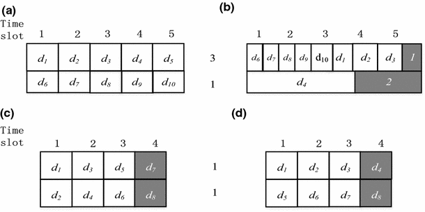
Clustering analysis
-
2.
\(\varvec{Wf}_{{\varvec{d}_{\varvec{i}} \varvec{ }}}\) To find the suitable channel bandwidth for a typical broadcast queue \(BQ_{i}\), the relationship between the data item priority and the broadcast efficiency is analyzed as follows. Given two particular channels, \(c_{1} \;{\text{and}}\;c_{2}\), where \(Bw_{1} = 1\) and \(Bw_{2} = 1\). Given a set of data items \(d_{1} \ldots d_{8}\), and the priority of \(d_{1} \ldots d_{4}\) is 5, while the priority of \(d_{5} \ldots d_{8}\) is 1. The data size of \(d_{1} \ldots d_{8}\) is 1. The broadcast cycle is 3 s. As shown in Fig. 4(c), \(d_{1} \ldots d_{4}\) are allocated into \(c_{1} {\text{and}} c_{2}\) evenly, as well as \(d_{5} \ldots d_{8}\), and then broadcast in order within \(c_{1} {\text{and}} c_{2}\). There is no time for \(d_{7} {\text{and}} d_{8}\) in this broadcast cycle. Fortunately, the data items with a high priority have broadcasting preference, and \(sumV_{k} = 22\). However, if one channel full of high priority data items will be harmful to the broadcast scheduling. Figure 4(d) shows the worst cast, where \(d_{4}\) with a high priority is not broadcast, and \(sumV_{k} = 18\). This approach is an effective way to allocate the data items into broadcast channels with priority equalization for broadcast scheduling.

In conclusion, clustering the data items with similar data sizes can reduce the bandwidth waste between two broadcast cycles and improve the bandwidth utilization. Allocating the data items into broadcast channels with priority equalization can help to increase the value of \(sumV_{k}\) in unit time by broadcast system.
4.2.2 Implementation of WASC
The process of WASC is as follows:
Step 1 Given a set \(D = \left\{ {d_{1} ,d_{2} , \ldots d_{i} , \ldots d_{N} } \right\}\) of N data items, the improved knowledge discovery by accuracy maximization (KODAMA) [42] algorithm is used to clustering D with the data item size. The details of the improved KODAMA algorithm are as follows: (1) let D as a dataset consist of N samples, and then assign each sample to a class defined in the class indicator vector \(T = \{ t_{1} ,t_{2} , \ldots t_{i} , \ldots t_{N} \}\), where \(t_{i}\) is the class label of the ith sample. If T is not predefined, each sample is assigned to a different class. A tenfold cross-validation procedure is performed on the basis of the classes defined in T using k-nearest neighbor (KNN), a supervised classifier. A record of the predicted class labels for each sample is then stored in \(Z_{T} = \left\{ {z_{1} ,z_{2} , \ldots z_{i} , \ldots z_{N} } \right\}\), where \(z_{i}\) is the predicted class label of the ith sample. The global accuracy is calculated by summing the number of correctly classified samples and dividing this number by the total number of samples. The obtained value is stored in the variable \(V_{T}\). (2) A new class indicator vector \(V = \left\{ {v_{1} ,v_{2} , \ldots v_{i} , \ldots v_{N} } \right\}\) is created by randomly swapping some of the class labels of the misclassified samples with the predicted class labels stored in \(Z_{T}\). A tenfold cross-validation procedure is performed on the basis of the classes defined in V. The relative accuracy value is then stored in \(A_{V }\) and the predicted class labels are stored in \(Z_{v} = \left\{ {z_{1} ,z_{2} , \ldots z_{i} , \ldots z_{N} } \right\}\). If \(A_{v} > A_{T}\), the value of \(A_{T}\) is changed to \(A_{v}\), vector T is changed to V, and vector \(Z_{T}\) is changed to \(Z_{v}\). Loop (2) until either \(A_{T}\) becomes equal to 100% or the maximum number of iterations is reached (the default value is 20).
Step 2 After Step 1, each data item is assigned to a class defined in T. The set D is clustered into several subsets \(G = \left\{ {g_{1} ,g_{2} , \ldots g_{i} , \ldots g_{{\frac{n}{2}}} } \right\}\), where \(g_{i }\) is the ith subset and n is even. A new subset vector \(FG = \{ g_{1,1} ,g_{1,2}\), \(g_{2,1} ,g_{2,2} , \ldots g_{i,1} ,g_{i,2} , \ldots g_{{\frac{n}{2},1}} ,g_{{\frac{n}{2},2}} \}\) is created by dividing all the sub-sets in G to balance the priority, where \(\left( {g_{i,1} ,g_{i,2} } \right)\) is created by dividing the \(g_{i}\) in G. The whole priority of \(g_{i}\) is calculated by summing the data items’ priority in \(g_{i}\). The obtained value is stored in the variable \(SW_{{g_{i} }}\). For \(d_{i}\) in \(g_{i}\), if \(SW_{{g_{i,1} }} > SW_{{g_{i,2} }}\), then allocate \(d_{i}\) to \(g_{i,1}\), else allocate \(d_{i}\) to \(g_{i,2}\) and recalculate the value of \(SW_{{g_{i,1} }} \;{\text{and}}\;SW_{{g_{i,2} }}\) by \(SW_{g} = \mathop \sum \limits_{{d_{i} \in g}} Wf_{{d_{i} }}\). Repeat this operation until all the data items have been allocated to \(g_{i,1}\) or \(g_{i,2}\).
Let N denote the overall number of data items in D, a tenfold cross-validation performed with KNN classifier has thus a time complexity of \(O(0.9 \times N^{2} )\), WASC consequently has a time complexity at most of \(O(0.9 \times N^{2} \times M)\), where the M is the number of times that the maximization of the cross validated accuracy is repeated.
4.3 Channel split algorithm
WASC is proposed to mine the characteristics of the data items. CSA is then proposed to find the most suitable broadcast channels and schedule the data items for broadcast. Splitting the original channel in real time according to the characteristics of the data items allows the broadcast to adapt to the varying mobile networks and improve the efficiency of the real-time ODDB system. The pseudo-code of CSA is described in detail in Table 1.
Let n denote the number of sub-channels and m denote the maximization number of data items in sun-channel, the time complexity for the CSA to calculates the bandwidth of sub-channels is \( O(n \times m) \), the time complexity for data assign is \( O(m) \). CSA consequently has a time complexity at most the of \( O(n \times m) \).
5 Experiments and analysis
To verify the advantages of the dynamic multi-channel architecture compared to single-channel architecture and fixed multi-channel architecture, extensive experiments were performed with different scheduling algorithms: RxW [10], GREEDY [13], TOSA [21], and OCSM. The RxW algorithm is based on single-channel architecture, and GREEDY and TOSA are based on fixed multi-channel architecture. OCSM is based on dynamic multi-channel architecture. We also attempted to compare OCSM with some of the state-of-the-art algorithms based on fixed multi-chan-nel architecture. However, GREEDY and TOSA are push-based algorithms. After studying a lot of literature, we found that there are very few pull-based algorithms based on fixed multi-channel architecture. We therefore changed GREEDY and TOSA to meet the restrictions of the pull-based property. The major parameters used in the experiments and the performance metrics are summarized in Section A. The experiments with the K value of OCSM were conducted under different distributions of data request and request deadline, which are detailed in Section B. The experiments with OCSM under different distributions of data request, request deadlines, and data size are described in Sections C, D, and E, respectively.
5.1 Experimental setup
5.1.1 Parameter settings
To simulate a real-world high-load on-demand data broadcast environment, the real access logs from the 1998 World Cup website [43] are used in this experiment. This log contains more than 7 million requests from more than 22,000 objects. The average request rate is 83 requests/s. In order to simplify the experiments, we processed the parameters before the experiments. The average deadline was set as 60 s, and assigned using the distributions of fixed, uni-form, and exponential. The average data item size was set as 1 unit and assigned using the distributions of normal, uniform, and Zipf. The request rate was set as 100 re-quests/s. The running time was set as 3600 s. In total, 360,000 requests were made in a run-time cycle. The num-ber of data items was set as 20,000. The number of sub-channels split by OCSM was ranged from 4 to 6, to ensure fair experi-ments, and the sub-channel number for RxW, GREEDY, and TOSA was set as 5. The parameter settings are listed in Table 2.
5.1.2 Performance metrics
For a real-time system, the LR is the primary performance metric, and is defined as the ratio of the number of requests missing their dead-lines to the total number of requests. It measures the capability of the system in meeting the deadlines of the requests. The primary goal of real-time ODDB scheduling is to minimize the LR. The total number of failed requests in the M broadcast cycles is \(L_{M} = \sum\nolimits_{k = 1}^{M} {\sum\nolimits_{i = 1}^{N} L } ed_{{d_{i} ,k}}\), where \(Led_{{d_{i} ,k}}\) is the number of failed re-quests in the k-th cycle. The total number of successful requests in the M broadcast cycles is \(S_{M} = \sum\nolimits_{k = 1}^{M} {\sum\nolimits_{i = 1}^{N} {S_{{d_{i} ,k}} } }\), where \(S_{{d_{i} ,k}}\) is the num-ber of successful requests in the k-th cycle. The LR is acquired by (5):
5.2 The K value of OCSM
OCSM extends the KNN algorithm [44] as a supervised classifier in step 1 of WASC. As we all know, the value of K directly affects the result of the KNN algorithm. Different distributions of deadline and data request lead to different characteristics of the data items. This section is devoted to determining the value of K under different distributions of deadline and data requests. It is generally believed that if N samples need to be clustered, the setting of \(K = \sqrt N\) can obtain the optimal results. In this experiment, we set the K values ranging from 10 to 100. Figure 5 shows the broadcast scheduling performance of different K values under different distributions of deadline (fixed distribution, uniform distribution, and exponential distribution) and data request (normal distribution, uniform distribution, and Zipf distribution) by LR, AAT, and NSC (the number of classes).


The performance of different K values under different distributions of deadline and data request (the x-axis is the value of K)
On the basis of the results shown in Fig. 5, we can make the following observations.
-
1.
With the incensement of K value, the NSC shows a declining trend. This phenomenon indicates that the K value is the determining factor of clustering result, the greater K value, the smaller the NSC.
-
2.
Under all the combination of different distributions of dead-line and data request, with the increments of K value, AAT is stable first, and then presents the rising trend, and then gradu-ally stabilized, which is because the accuracy of supervised classifier reduces with the increments of K value. It results in a poor broadcast performance.
-
3.
When the K value increased from 10 to 30, LR shows a slight decline trend. However, when the K value increased from 35 to 45, LR increased rapidly. Then, LR remains at a high status.
Through the above analysis, we conclude that the value of K has a significate influence on the performance of OCSM. For the optimal OCSM performance, the suggestions for the value of K under different deadline and data request distributions based on the metrics of LR, AAT and NSC are given.
There are strict timing constraints for real-time ODDB, request with a specific deadline will become invalid if the server fails to response it within the deadline. To maximum satisfy the requests of the clients, the LR must be primary consideration for the optimal K value selection. To ensure a high quality of service, the AAT should be considered as another important metric since it represents the wait of clients. Finally, the NSC is less important compare to LR and AAT since it could be solved by improving the computing ability of the server. Therefore, the strategy of optimal K value selection is presented in Strategy 1.

Based on the optimal K value selection strategy, the suggested optimal value of K and the corresponding number of sun-channels N as shown in Table 3.
5.3 Performance of OCSM under different data request distributions
Experiments were carried out to compare the performance of OCSM to RxW, GREEDY, and TOSA under different data request distributions (Zipf distribution, uniform distribution, normal distribution). The probability density function of the data request under a Zipf distribution is \(p_{i} = \frac{{{\raise0.7ex\hbox{$1$} \!\mathord{\left/ {\vphantom {1 i}}\right.\kern-0pt} \!\lower0.7ex\hbox{$i$}}^{\theta } }}{{\mathop \sum \nolimits_{i = 1}^{20000} {\raise0.7ex\hbox{$1$} \!\mathord{\left/ {\vphantom {1 i}}\right.\kern-0pt} \!\lower0.7ex\hbox{$i$}}^{\theta } }}, 1 \le i \le 20000,\) where \(p_{i }\) the request probability of is \(d_{i}\). We set \(\theta = 1\). The deadline was set as a uniform distribution, with an average value of 60 s. The data item size of RxW and GREEDY was set as 1 unit. OCSM and TOSA were run under a uniform distribution, with the average value set as 1 unit. The K value in OCSM was set as 25 under a Zipf distribution, 18 under a uniform distribution, and 11 under a normal distribution. The experimental results are shown in Fig. 6.

LR under different data request distributions
As illustrated in Fig. 6, the LR of all algorithms increases greatly as the request arrival rate increases from 20 to 80, and they increase slightly as the request arrival rate increases from 80 to 180. This agrees with the intuition that the higher the request rate is, the higher the system load is, and the higher LR is. Specifically, the conclusions are made as follows.
-
1.
The LR of the push-based algorithms (GREEDY and TOSA) are higher than pull-based at a low request rate. This is because a push-based algorithm relies on the priori knowledge of the clients’ requests. When the requests cover most of the data items of push-based broadcast, the performance of GREEDY and TOSA are better than before.
-
2.
The highest LR overall occur for uniform request distribution and the lowest LR for Zipf distribution because the only a small set of data items are accessed frequently under Zipf.
-
3.
OCSM achieve the lowest LR under Zipf distribution, which confirms that OCSM clusters more accurate with obvious data characteristics. At the low request rate for the normal and uniform data request, the OCSM has the lowers LR, while at the higher request rate, the performance of OCSM is similar to TOSA.
-
4.
By comparing the performance of each algorithm in the three situations, we can see that the LR of all the algorithms are greatest for the uniform distribution and the smallest for Zipf distribution. This can be attributed to the fact that it is more likely for a selected data item to satisfy multiple requests before their deadlines as the access pattern becomes more skewed. Under these three request distribution, OCSM generally performs best, especially under a Zipf distribution, where the characteristics of the data items are obvious.
5.4 Performance of OCSM under different request deadline distributions
Experiments were carried out to compare the performance of OCSM to that of RxW, GREEDY, and TOSA under different request deadline distributions (uniform distribution, exponential distribution, and fixed distribution). The data item size of RxW and GREEDY was fixed as 1 unit. OCSM and TOSA were run under a uniform distribution, with the average value set as 1 unit. The data request distribution was set as a Zipf distribution, and the request rate was set as 100 requests/s. The K value in OCSM was set as 18 under a uniform distribution, 17 under an exponential distribution, and 17 under a fixed distribution. The experimental results are shown in Fig. 7.

Loss rates under different request deadline distributions
As illustrated in Fig. 7, we can make the following observation:
-
1.
The LR of all algorithms decrease greatly as the deadline increases from 10 to 85, and they decrease slightly as the deadline increases from 85 to 200. This result is expected because the longer deadline is, the lower the timing constraint is, and the greater the possibility the request will be satisfied. Specifically, the conclusions are made as follows.
-
2.
With the extension of the request deadline, the LR of the two push-based scheduling algorithms, GREEDY and TOSA, reduces more slowly than for the two pull-based algorithms. This is because push-based algorithms considers a static data access pattern and disseminates data items cyclically according to a pre-defined schedule. Therefore, even if the deadline is extended, the LR remains high.
-
3.
The LR for the exponential deadlines is the greatest, because of the possibility of occurrence of deadline I will decrease with the increasing value of I under the exponential deadline distribution. To some extent, the characteristic of data items are more obvious in that case, therefore, OCSM is still able to achieve the lowest LR.
-
4.
OCSM has lowest LR while in the uniform, because the deadline distribution is relatively concentrated and the characteristics of data items are obvious, which makes the OCSM clustering more accurate. While, when the request deadline is under a fixed distribution, OCSM has no advantage in this case, the LR of OCSM is higher than TOAS.
5.5 The performance of OCSM under a fixed distribution of data item size
Experiments were carried out to compare the performance of OCSM with that of RxW, GREEDY, and TOSA under a fixed distribution of data item size. The data request distribution was set as a Zipf distribution, and the request rate was set as 100 requests/s. The request deadline distribution was set as a uniform distribution, with an average value of 60 s. The K value in OCSM was set as 18. On the basis of the results shown in Fig. 8, we can make the following observations:

Loss rates under a fixed distribution of data item size
-
1.
Because RxW and GREEDY do not consider the data item size, their performances are poor. With the increase of the data item size, the LR of RxW and GREEDY increases rapidly.
-
2.
TOSA and OCSM consider the value of the data item, and data items with a high value have a high broadcast priority. With the increase of the data item size, they still obtain a lower LR, and the performance of OCSM is better than TOSA.
6 Conclusions and future work
The disadvantage of the single-channel architecture and fixed multi-channel architecture lies in the fact that the broadcast channel is fixed, so that it cannot adjust flexibly to adapt to real-time client requests. In this paper, to overcome this disadvantage, we have studied adaptive multi-channel on-demand data broadcasting (ODDB) and proposed an adaptive channel split and allocation method named the optimized channel split method (OCSM). Extensive experiments were conducted to evaluate the performance of OCSM, allowing a number of conclusions to be drawn as follows.
-
1.
In the case of the characteristics of the data items being obvious, OCSM performs better than the other state-of-the-art methods.
-
2.
Compared to the single-channel broadcast scheduling algorithms, OCSM applies the adaptive channel split strategy, which can make full use of the parallel broadcasting characteristic of the multi-channel system.
-
3.
Compared to the fixed multi-channel broadcast scheduling algorithms, OCSM has a stronger adaptability and can perform better under different data distributions.
Our future work will mainly focus on an index strategy based on OCSM, with the aim being to reduce the tuning time of clients, and to consider the situation where the client request contains multiple data items.
References
Li, L. J., Liu, H. F., Yang, Z. Y., et al. (2010). Broadcasting methods in vehicular ad hoc networks. Journal of Software, 21(7), 1620–1634.
Wang, H., Xiao, Y., & Shu, L. C. (2012). Scheduling periodic continuous queries in real-time data broadcast environments. IEEE Transactions on Computers, 61(9), 1325–1340.
Jung, H., Chung, Y., & Liu, L. (2012). Processing generalized k-nearest neighbor queries on a wireless broadcast stream. Information Sciences, 188(4), 64–79.
Yu, C., Yao, D., Li, X., Zhang, Y., Yang, L., Xiong, N., et al. (2012). Location-aware private service discovery in pervasive computing environment. Information Sciences, 230(5), 78–93.
Simunic, T., Boyd, S., & Glynn, P. (2004). Managing power consumption in networks on chips. IEEE Transactions on Very Large Scale Integration Systems, 2(1), 96–107.
Cheng, H. J., Huang, X. B., & Xiong, N. X. (2014). Minimum-energy broadcast algorithm for wireless sensor networks with unreliable communication. Journal of Software, 25(5), 1101–1112.
Zhao, R. Q., Liu, Z. J., & Wen, A. J. (2009). An efficient energy-saving broadcast mechanism for wireless sensor networks. Acta Electronica Sinica, 37(11), 2457–2462.
Waluyo, A., Srinlvasan, B., Taniar, D., et al. (2005). Incorporating global index multi data placement scheme for multi channels mobile broadcast environment. Lecture Notes in Computer Science, 3824, 755–764.
Lee, S., Carney, D. P., Zdonik, S. (2003). Index hint for on-demand broadcasting. In Proceedings of the 19th IEEE international conference on data engineering (pp. 726–728).
Aksoy, D., & Franklin, M. (1999). RxW: A scheduling approach for large scale on-demand data broadcast. IEEE/ACM Transactions on Networking, 7(6), 846–860.
Wu, X., & Lee, V. C. S. (2005). Wireless real-time on-demand data broadcast scheduling with dual deadlines. Journal of Parallel and Distributed Computing, 65(6), 714–728.
Saxena, N., & Pinottti, M. (2005). On-line balanced k-channel data allocation with hybrid schedule per channel. In Proceedings of the 6th International conference on mobile data management (pp. 239–246). ACM.
Anticaglia, S. S., Barsi, F., Bertossi, A. A., et al. (2008). Efficient heuristics for data broadcasting on multiple channels. Wireless Networks, 14(2), 219–231.
Waluyo, A., Srinlvasan, B., Taniar, D., et al. (2005). Incorporating global index multi data placement scheme for multi channels mobile broadcast environment. Lecture Notes in Computer Science, 3824, 755–764.
Chung, Y., Chen, C., & Lee, C. (2008). Design and performance evaluation of broadcast algorithms for time-constrained data retrieval. IEEE Transactions on Knowledge and Data Engineering, 18(11), 1526–1543.
Lee, W., Hu, Q., & Lee, D. (1999). A study on channel allocation for data dissemination in mobile computing environments. Mobile Networks and Applications, 1(2), 117–129.
Gao, X., Yang, Y., Chen, G., et al. (2016). Global optimization for multi-channel wireless data broadcast with AH-tree indexing scheme. IEEE Transactions on Computers, 65(7), 2104–2117.
Lim, J. H., Naito, K., Yun, J. H. et al. (2015). Revisiting overlapped channels: Efficient broadcast in multi-channel wireless networks. In 2015 IEEE conference on computer communications (INFOCOM). IEEE.
Nawaz Ali, G. G. M., Lee, V. C. S., Chan, E., et al. (2014). Admission control-based multichannel data broadcasting for real-time multi-item queries. IEEE Transactions on Broadcasting, 60(4), 589–605.
Hu, C., & Chen, M. (2002). Adaptive balanced hybrid data delivery for multi-channel data broadcast. In Proceedings of IEEE international conference on communications (pp. 960–964).
Zheng, B., Wu, X., Jin, X., et al. (2005). TOSA: A near-optimal scheduling algorithm for multi-channel data broadcast. In Proceedings of the 6th international conference on mobile data management (pp. 20–37). ACM.
Moulahi, T., Nasri, S., & Guyennet, H. (2012). Broadcasting based on dominated connecting sets with MPR in a realistic environment for WSNS & ad hoc. Journal of Network and Computer Applications, 35(6), 1720–1727.
Zheng, Q., Zheng, K., Zhang, H., et al. (2016). Delay-optimal virtualized radio resource scheduling in software-defined vehicular networks via stochastic learning. IEEE Transactions on Vehicular Technology, 65(10), 7857–7867.
Ma, W. M., Zhang, H. J., Wen, X. M., et al. (2012). A novel QoS guaranteed cross-layer scheduling scheme for downlink multiuser OFDM systems. Applied Mechanics and Materials, 182–183, 1352–1357.
Utility-Based Cross-Layer Multiple Traffic Scheduling for MU-OFDMA. (2012). Advances in Information Sciences and Service Sciences, 3(8), 122–131.
Zhang, H., Jiang, C., Beaulieu, N. C., Chu, X., Wen, X., & Tao, M. (2014). Resource allocation in spectrum-sharing OFDMA femtocells with heterogeneous services. IEEE Transactions on Communications, 62(7), 2366–2377.
Zhang, H., Jiang, C., Beaulieu, N. C., Chu, X., Wang, X., & Quek, T. Q. (2015). Resource allocation for cognitive small cell networks: A cooperative bargaining game theoretic approach. IEEE Transactions on Wireless Communications, 14(6), 3481–3493.
Xuan, P., et al. (1997). Broadcast on demand: efficient and timely dissemination of data in mobile environments. In Proceedings of the third IEEE real-time technology and applications symposium (pp. 350–350). IEEE.
Fang, Q., Vrbsky, S., Dang, Y., & Ni, W. (2004). A pull-based broadcast algorithm that considers timing constraints. In Proceedings of the 2004 international conference on parallel processing workshops (pp. 46–53).
Kalyanasundaram, B., & Velauthapillai, M. (2003). On-demand broadcasting under deadline. In Proceedings of the 11th annual European symposium on algorithms (pp. 313–324).
Ng, J., Lee, V., & Hui, C. (2008). Client-side caching strategies and on-demand broadcast algorithms for real-time information dispatch system. IEEE Transactions on Broadcasting, 54(1), 24–35.
Dykeman, H., & Wong, J. (1988). A performance study of broadcast information delivery systems. In Seventh annual joint conference of the IEEE computer and communications societies (pp. 739–745).
Dewri, R., Ray, I., Ray, I., & Whitley, D. (2008). Optimizing on-demand data broadcast scheduling in pervasive environments. In Proceedings of the 11th international conference on extending database technology: Advances in database technology, Nantes, France (pp. 559–569).
Hu, W., Fan, C., Luo, J., et al. (2015). An on-demand data broadcasting scheduling algorithm based on dynamic index strategy. Wireless Communications and Mobile Computing, 15(5), 947–965.
Hu, W., Xia, C., Du, B., et al. (2015). An on-demanded data broadcasting scheduling considering the data item size. Wireless Networks, 21(1), 35–56.
Hu, W., Qiu, Z., Wang, H., & Yan, L. (2016). A real-time scheduling algorithm for on-demand wireless xml data broadcasting. Journal of Network and Computer Applications, 68, 151–163.
Ma, W. M. (2012). Utility-based fairness power control scheme in OFDMA femtocell networks. Journal of Electronics and Information Technology, 34(10), 2287–2292.
Zhang, H., Jiang, C., Mao, X., et al. (2016). Interference-limited resource optimization in cognitive femtocells with fairness and imperfect spectrum sensing. IEEE Transactions on Vehicular Technology, 65(3), 1.
Zhang, H., Chu, X., & Wen, X. (2013). 4G Femtocells: Resource Allocation and Interference Management. Berlin: Springer.
Lv, J., Lee, V. C. S., Li, M., et al. (2012). Admission control and channel allocation of multi-item requests for real-time data broadcast. In 2013 IEEE 19th international conference on embedded and real-time computing systems and applications (pp. 202–211). IEEE.
Viswanathan, S., & Imielinski, T. (1995). Pyramid broadcasting for video on-demand service. In Proceedings of SPIE (pp. 66–66).
Stefano, C., Claudio, L., & Leonardo, T. (2014). Knowledge discovery by accuracy maximization. Proceedings of the National Academy of Sciences of the United States of America, 111(14), 5117–5122.
World Cup 98 Web Site Access Logs. (1998). http://ita.ee.lbl.gov/html/contribute/WorldCup.html[EB/OL].
Lu, F., Du, N., & Wen, C. L. (2012). A fuzzy-evidential k nearest neighbor classification algorithm. Acta Electronica Sinica, 40(12), 2390–2395.
Acknowledgements
This work is partially supported by National Natural Science Foundation of China (61572369); National Natural Science Foundation of Hubei Province (2015CFB423); Wuhan Major Science and Technology Program (2015010101010023).
Author information
Authors and Affiliations
Corresponding authors
Rights and permissions
About this article

Cite this article
Hu, W., Qiu, Z., Nie, C. et al. OCSM: an optimized channel split method—towards real-time and on-demand data broadcast scheduling. Wireless Netw 25, 861–874 (2019). https://doi.org/10.1007/s11276-017-1598-7
Published:
Issue Date:
DOI: https://doi.org/10.1007/s11276-017-1598-7