
Abstract
Recent advances in 3D shape analysis and recognition have shown that heat diffusion theory can be effectively used to describe local features of deforming and scaling surfaces. In this paper, we show how this description can be used to characterize 2D image patches, and introduce DaLI, a novel feature point descriptor with high resilience to non-rigid image transformations and illumination changes. In order to build the descriptor, 2D image patches are initially treated as 3D surfaces. Patches are then described in terms of a heat kernel signature, which captures both local and global information, and shows a high degree of invariance to non-linear image warps. In addition, by further applying a logarithmic sampling and a Fourier transform, invariance to photometric changes is achieved. Finally, the descriptor is compacted by mapping it onto a low dimensional subspace computed using Principal Component Analysis, allowing for an efficient matching. A thorough experimental validation demonstrates that DaLI is significantly more discriminative and robust to illuminations changes and image transformations than state of the art descriptors, even those specifically designed to describe non-rigid deformations.
1 Introduction
Building invariant feature point descriptors is a central topic in computer vision with a wide range of applications such as object recognition, image retrieval and 3D reconstruction. Over the last decade, great success has been achieved in designing descriptors invariant to certain types of geometric and photometric transformations. For instance, the SIFT descriptor (Lowe 2004) and many of its variants (Bay et al. 2006; Ke and Sukthankar 2004; Mikolajczyk and Schmid 2005; Morel and Yu 2009; Tola et al. 2010) have been proven to be robust to affine deformations of both spatial and intensity domains. In addition, affine deformations can effectively approximate, at least on a local scale, other image transformations including perspective and viewpoint changes. However, as shown in Fig. 1, this approximation is no longer valid for arbitrary deformations occurring when viewing an object that deforms non-rigidly.

Comparing DaLI against SIFT (Lowe 2004), DAISY (Tola et al. 2010), LIOP (Wang et al. 2011) and GIH (Ling and Jacobs 2005). Input images correspond to different appearances of the object shown in the reference images, under the effect of non-rigid deformations and severe changes of illumination. Colored circles indicate the match has been correctly found among the first \(n\) top candidates, where \(n\le 10\) is parameterized by the legend on the right. A feature is considered as mismatched when \(n>10\) and we indicate this with a cross. Note that the DaLI descriptor yields a significantly larger number of correct matches
In order to match points of interest under non-rigid image transformations, recent approaches propose optimizing complex objective functions that enforce global consistency in the spatial layout of all matches (Cheng et al. 2008; Cho et al. 2009; Leordeanu and Hebert 2005; Sanchez et al. 2010; Serradell et al. 2012; Torresani et al. 2008). Yet, none of these approaches explicitly builds a descriptor that goes beyond invariance to affine transformations. An interesting exception is Ling and Jacobs (2005), that proposes embedding the image in a 3D surface and using a Geodesic Intensity Histogram (GIH) as a feature point descriptor. However, while this approach is robust to non-rigid deformations, its performance drops under light changes. This is because a GIH considers deformations as one-to-one image mappings where image pixels only change their position but not the magnitude of their intensities.
To overcome the inherent limitation of using geodesic distances, we propose a novel descriptor based on the Heat Kernel Signature (HKS) recently introduced for non-rigid 3D shape recognition (Gębal et al. 2009; Rustamov 2007; Sun et al. 2009), and which besides invariance to deformation, has been demonstrated to be robust to global isotropic (Bronstein and Kokkinos 2010) and even affine scalings (Raviv et al. 2011). In general, the HKS is particularly interesting in our context of images embedded on 3D surfaces, because illumination changes produce variations on the intensity dimension that can be seen as local anisotropic scalings, for which Bronstein and Kokkinos (2010) still shows a good resilience.
Our main contribution is thus using the tools of diffusion geometry to build a descriptor for 2D image patches that is invariant to non-rigid deformations and photometric changes. To construct our descriptor we consider an image patch \(P\) surrounding a point of interest, as a surface in the \((x,y,\beta I(\mathbf {x}))\) space, where \((x,y)\) are the spatial coordinates, \(I(\mathbf {x})\) is the intensity value at \((x,y)\), and \(\beta \) is a parameter which is set to a large value to favor anisotropic diffusion and retain the gradient magnitude information. Drawing inspiration from the HKS (Gębal et al. 2009; Sun et al. 2009), we then describe each patch in terms of the heat it dissipates onto its neighborhood over time. To increase robustness against 2D and intensity noise, we use multiple such descriptors in the neighborhood of a point, and weigh them by a Gaussian kernel. As shown in Fig. 1, the resulting descriptor (which we call DaLI, for Deformation and Light Invariant) outperforms state-of-the-art descriptors in matching points of interest between images that have undergone non-rigid deformations and photometric changes.
A preliminary version of this paper was already published in Moreno-Noguer (2011). In the current work, we propose alternatives to both alleviate the high cost of the heat kernel computation and to reduce the dimensionality of the descriptor. More specifically, while in Moreno-Noguer (2011) the 3D embedding was performed considering a mesh with a uniform distribution of vertices in the \((x,y)\) domain, here we investigate topologies with varying vertex densities. This allows reducing the effective size of the underlying mesh, and hence to speed up the DaLI computation time by a factor of over \(4\). In addition, we have also compacted the size of the final descriptor by a factor of \(50\times \) using a Principal Component Analysis (PCA) for dimensionality reduction. As a result, the descriptor we propose here can be computed and matched much faster when compared to Moreno-Noguer (2011), while preserving the discriminative power. For evaluation, we acquired a challenging dataset that contains 192 pairs of real images, manually annotated, of diverse materials under different degrees of deformation and being illuminated by very different illumination conditions. Fig. 1-left shows two samples of our dataset. We believe this is the first deformation and illumination dataset for evaluating image descriptors using real-world objects, and have made the dataset along with the code of the DaLI descriptor publicly availableFootnote 1.
2 Related Work
The SIFT descriptor (Lowe 2004) has become the main reference among feature point descriptors, showing great success in capturing local affine deformations including scaling, rotation, viewpoint change and certain lighting changes. Since it is relatively slow to compute, most of the subsequent works have focused on developing faster descriptors (Bay et al. 2006; Calonder et al. 2012; Ke and Sukthankar 2004; Mikolajczyk and Schmid 2005; Tola et al. 2010). Scale and rotation invariance has also been demonstrated in Kokkinos et al. (2012) using a combination of logarithmic sampling and multi-scale signal processing, although that requires large image patches which make the resulting descriptor more sensitive to other deformations. Indeed, as discussed in Vedaldi and Soatto (2005), little effort has been devoted to building descriptors robust to more general deformations.
The limitations of the affine-invariant descriptors when solving correspondences between images of objects that have undergone non-rigid deformations are compensated by enforcing global consistency, both spatial and photometric, among all features (Belongie et al. 2002; Berg et al. 2005; Cheng et al. 2008; Cho et al. 2009; Leordeanu and Hebert 2005; Sanchez et al. 2010; Serradell et al. 2012; Torresani et al. 2008), or introducing segmentation information within the descriptor itself (Trulls et al. 2013, 2014). In any event, none of these methods specifically handles the non-rigid nature of the problem, and they rely on solving complex optimization functions for establishing matches.
An alternative approach is to directly build a deformation invariant descriptor. With that purpose, recent approaches in two-dimensional shape analysis have proposed using different types of intrinsic geometry. For example, Bronstein et al. (2007), Ling and Jacobs (2007) define metrics based on the inner-distance, and Ling et al. (2010) proposes using geodesic distances. However, all these methods require the shapes to be segmented out from the background and represented by binary images, which is difficult to do in practice. In Ling and Jacobs (2005), it was shown that geodesic distances, in combination with an appropriate 3D embedding of the image, were adequate to achieve deformation invariance in intensity images. Nonetheless, this method assumes that pixels only change their image locations and not their intensities and, as shown in Fig. 1, is prone to failure under illumination changes.
There have also been efforts to build illumination invariant descriptors. Such works consider strategies based on intensity ordering and spatial sub-division (Fan et al. 2012; Gupta and Mittal 2007, 2008; Gupta et al. 2010; Heikkilä et al. 2009; Tang et al. 2009; Wang et al. 2011). While these approaches are invariant to monotonically increasing intensity changes, their success rapidly falls when dealing with photometric artifacts produced by complex surface reflectances or strong shadows.
The DaLI descriptor we propose can simultaneously handle such relatively complex photometric and spatial warps. Following Ling and Jacobs (2005), we represent the images as 2D surfaces embedded in the 3D space. This is in fact a common practice, although it has been mostly employed for low level vision tasks such as image denoising (Sochen et al. 1998; Yezzi 1998) or segmentation (Yanowitz and Bruckstein 1989). The fundamental difference between our approach and Ling and Jacobs (2005) is that we then describe each feature point on the embedded surface considering the heat diffusion over time (Gębal et al. 2009; Lévy 2006; Sun et al. 2009) instead of using a Geodesic Intensity Histogram. As we will show in the results section this yields substantially improved robustness, especially to illumination changes. Heat diffusion theory has been used by several approaches for the analysis of 3D textured (Kovnatsky et al. 2011) and non-textured shapes (Goes et al. 2008; Lévy 2006; Reuter et al. 2006; Rustamov 2007), but to the best of our knowledge, it has not been used before to describe patches in intensity images.
One of the main limitations of the methods based on the heat diffusion theory is the high complexity cost they require. The bottleneck of their computation lies on an eigendecomposition of a \(n_v\times n_v\) Laplacian matrix (see Fig. 3), where \(n_v\) is the number of vertices of the underlying mesh. This has been addressed by propagating the eigenvectors across different mesh resolutions (Shi et al. 2006; Wesseling 2004) or using matrix exponential approximations (Vaxman et al. 2010). In this paper, an annular multiresolution grid will be used to improve the efficiency of the DaLI computation. Additionally, PCA will be used to reduce the dimensionality of the original DaLI descriptor (Moreno-Noguer 2011), hence speeding up the matching process as well.
3 Deformation and Light Invariant Descriptor
Our approach is inspired by current methods (Gębal et al. 2009; Sun et al. 2009) that suggest using diffusion geometry for 3D shape recognition. In this section we show how this theory can be adapted to describe 2D local patches of images that undergo non-rigid deformations and photometric changes. A general overview of the different steps needed to compute the DaLI and DaLI-PCA descriptors can be seen in Fig. 2 and are explained more in detail below.

Flowchart of the algorithm used to calculate the DaLI and DaLI-PCA descriptors. The percentages below each of the steps indicate the total amount of the contribution of that step to the computation time. Observe that 99 % of the computation time corresponds to the Heat Kernel Signature calculation and specifically almost entirely to the eigendecomposition of the Laplace–Beltrami operator
3.1 Invariance to Non-Rigid Deformations
Let us assume we want to describe a 2D image patch \(P\), of size \(S_P\times S_P\) and centered on a point of interest \(\mathbf {p}\). In order to apply the diffusion geometry theory to intensity patches we regard them as 2D surfaces embedded in 3D space (Fig. 3 bottom-left). More formally, let \(f: P\rightarrow M\) be the mapping of the patch \(P\) to a 3D Riemannian manifold \(M\). We explicitly define this mapping by:
where \(I(\mathbf {x})\) is the pixel intensity at \(\mathbf {x}=(x,y)^\top \), and \(\beta \) is a parameter that, as we will discuss later, controls the amount of gradient magnitude preserved in the descriptor.
Several recent methods (Gębal et al. 2009; Lévy 2006; Reuter et al. 2006; Rustamov 2007; Sun et al. 2009) have used the heat diffusion geometry for capturing the local properties of 3D surfaces and performing shape recognition. Similarly, we describe each patch \(P\) based on the heat diffusion equation over the manifold \(M\):
where \(\Delta _M\) is the Laplace–Beltrami operator, a generalization of the Laplacian to non-Euclidean spaces, and \(u(\mathbf {x},t)\) is the amount of heat on the surface point \(\mathbf {x}\) at time \(t\).
The solution \(k(\mathbf {x},\mathbf {y},t)\) of the heat equation with an initial heat distribution \(u_o(\mathbf {x},t)=\delta (\mathbf {x}-\mathbf {y})\) is called the heat kernel, and represents the amount of heat that is diffused between points \(\mathbf {x}\) and \(\mathbf {y}\) at time \(t\), considering a unit heat source at \(\mathbf {x}\) at time \(t=0\). For a compact manifold \(M\), the heat kernel can be expressed by following spectral expansion (Chavel 1984; Reuter et al. 2006):
where \(\{\lambda _i\}\) and \(\{\varvec{\phi }_i\}\) are the eigenvalues and eigenfunctions of \(\Delta _M\), and \(\varvec{\phi }_i(\mathbf {x})\) is the value of the eigenfunction \(\varvec{\phi }_i\) at the point \(\mathbf {x}\). Based on this expansion, Sun et al. (2009) proposes describing a point \(\mathbf {p}\) on \(M\) using the Heat Kernel Signature
which is shown to be isometrically-invariant, and adequate for capturing both the local properties of the shape around \(\mathbf {p}\) (when \(t\rightarrow 0\)) and the global structure of \(M\) (when \(t\rightarrow \infty \)).
However, while on smooth surfaces the HKS of neighboring points are expected to be very similar, when dealing with the wrinkled shapes that may result from embedding image patches, the heat kernel turns to be highly unstable along the spatial domain (Fig. 3 bottom-right). This makes the HKS particularly sensitive to noise in the 2D location of the keypoints. To handle this situation, we build the descriptor of a point \(\mathbf {p}\) by concatenating the HKS of all points \(\mathbf {x}\) within the patch \(P\), properly weighted by a Gaussian function of the distance to the center of the patch. We therefore define the following Deformation Invariant (DI) descriptor:
where \(G(\mathbf {x};\mathbf {p},\sigma )\) is a 2D Gaussian function centered on \(\mathbf {p}\) having a standard deviation \(\sigma \), evaluated at \(\mathbf {x}\). Note that for a specific time instance \(t\), \({\text {DI}}(\mathbf {p},t)\) is a \(S_P \times S_P \) array.
The price we pay for achieving robustness to 2D noise is an increase of the descriptor size. That is, if \({\text {HKS}}(\mathbf {p},t\)) is a function defined on the temporal domain \(\mathbb {R}^+\) discretized into \(n_t\) equidistant intervals, the complete DI descriptor \({\text {DI}}(\mathbf {p})=[{\text {DI}}(\mathbf {p},t_1), \ldots , {\text {DI}}(\mathbf {p},t_{n_t})]\) will be defined on \(S_P \times S_P \times n_t\), the product of the spatial and temporal domains. However, note that for our purposes this is still feasible, because we do not need to compute a descriptor for every pixel of the image, but just for a few hundreds of points of interest. Furthermore, as we will next discuss, the descriptor may be highly compacted if we represent it in frequency domain instead of time domain and even further compacted by using dimensionality reduction techniques such as principal component analysis (PCA).

DaLI descriptor. Our central idea is to embed image patches in 3D surfaces and describe them based on heat diffusion processes. We represent the heat diffusion as a stack of images in the frequency domain. The top images show various slices of our descriptor for two different patches. The bottom-right graph depicts the value of the descriptor for the pixels marked by color circles in the upper images. Note that corresponding pixels have very similar signatures. However, the signature may significantly change from one pixel to its immediate neighbor. For instance, \(\mathbf {z}_2\) is at one pixel distance from \(\mathbf {x}_2\), but their signatures are rather different. As a consequence, using the signature of a single point as a descriptor is very sensitive to 2D noise in the feature detection process. We address this by simultaneously considering the signature of all the pixels within the patch, weighted by a Gaussian function of the distance to the center of the patch
3.2 Invariance to Illumination Changes
An inherent limitation of the descriptor introduced in Eq. (4) is that it is not illumination invariant. This is because light changes scale the manifold \(M\) along the intensity axis, and the HKS is sensitive to scaling. It can be shown that an isotropic scaling of the manifold \(M\) by a factor \(\alpha \), scales the eigenvectors and eigenvalues of Eq. (2) by factors \(1/\alpha \) and \(1/\alpha ^2\), respectively (Reuter et al. 2006). The HKS of a point \(\alpha \mathbf {p}\in \alpha M\) can then be written as
which is an amplitude and time scaled version of the original HKS.
Nonetheless, under isotropic scalings, several alternatives have been proposed to remove the dependence of the HKS on the scale parameter \(\alpha \). For instance, Reuter et al. (2006) suggests normalizing the eigenvalues in Eq. (2). In this paper we followed Bronstein and Kokkinos (2010), that applies three consecutive transformations on the HKS. First, the time-dimension is logarithmically sampled, which turns the time scaling into a time-shift, that is, the right-hand side of Eq. (5) begets \(\alpha ^{-2}{\text {HKS}}(\mathbf {p},-2\log \alpha +\log t)\). Second, the amplitude scaling factor is removed by taking logarithm and derivative w.r.t. \(\log t\). The Heat Kernel then becomes \(\frac{\partial }{\partial \log t}\log {\text {HKS}}(\mathbf {p},-2\log \alpha +\log t)\). The time-shift term \(-2\log \alpha \) is finally removed using the magnitude of the Fourier transform, which yields \({\text {SI-HKS}}(\mathbf {p},w)\), a scale invariant version of the original HKS in the frequency domain. In addition, since most of the signal information is concentrated in the low-frequency components, the size of the descriptor can be highly reduced compared to that of \({\text {HKS}}(\mathbf {p},t)\) by eliminating the high-frequency components past a certain frequency threshold \(w_{max}\).
As we will show in the results section, another advantage of the SI-HKS signature is that although it is specifically designed to remove the dependence of the HKS on isotropic scalings, it is quite resilient to anisotropic transformations, such as those produced by photometric changes that only affect the intensity dimension of the manifold \(M\). Thus, we will use this signature to define our Deformation and Light Invariant (DaLI) descriptor:
Again, the full \({\text {DaLI}}(\mathbf {p})\) descriptor is defined as a concatenation of \(w_{max}\) slices in the frequency domain, each of size \(S_P \times S_P\).
Figure 3-top shows several DaLI slices at different frequencies for a patch and a deformed version of it. As said above, observe that most of the signal is concentrated in the low frequency components. In Fig. 4 we compare the sensitivity of the DI and DaLI descriptors to deformation and light changes, simulated here by a uniform scaling of the intensity channel. Note that DaLI, in contrast to DI, remains almost invariant to light changes, and it also shows a better performance under deformations. In the results section, we will show that this invariance is also accompanied by a high discriminability, yielding significantly better results in keypoint matching than existing approaches.

Invariance of the DaLI and DI descriptors to non-rigid deformations and illumination changes. Top row and left column images: Different degrees of deformation and light changes applied on the top left reference patch \(P_0\). Deformations are applied according to a function \({\text {Def}}(\cdot )\in \left\{ {\text {Def}}0,\ldots ,{\text {Def}}11\right\} \), where \({\text {Def}}11\) corresponds to the maximal deformation. Light changes are produced by scaling the intensity of \(P_0\) by a gain \( g\in \left[ 0,1\right] \). Bottom Graph: Given a deformation \({\text {Def}}(\cdot )\) and a gain factor \(g\), we compute the percentage of change of the DI descriptor by \(\Vert {\text {DI}}(P_0)-{\text {DI}}({\text {Def}}(gP_0))\Vert /\Vert {\text {DI}}(P_0)\Vert \). The percentage of change for DaLI is computed in a similar way. Observe that DaLI is much less sensitive than DI, particularly to illumination changes
In order to get deeper insight about the properties of the DaLI descriptor, we have further evaluated the HKS and SI-HKS descriptor variants on a synthetic experiment, in which we have rendered various sequences of images of a textured 3D wave-like mesh under different degrees of deformation and varying illumination conditions. The surface’s reflectance is assumed to be Lambertian and the light source is moved near the surface, producing lighting patterns that combine both shading and the effects of the inverse-square falloff law.
We have analyzed four particular situations: Def.+Ill., varying both deformation and the light source position; Def., varying deformation and keeping the light source at infinity; Ill. (Def.), starting with a largely deformed state which is kept constant along the sequence and varying the light source position; and Ill. (No Def.), varying the light source position while keeping the surface flat. The mesh deformation in the first two sequences, corresponds to a sinusoidal warp, in which the amplitude of the deformation increases with the frame number. The varying lighting conditions in all experiments except the second, are produced by smoothly moving the light source on a hemisphere very close to the surface. Two frames from each of these sequences are shown in the top-left of Fig. 5.

Evaluation of the descriptor robustness on synthetic sequences. In the top-left we show two sample images (the reference image and one specific frame) from all four different scenarios we consider. In the top-right we show an 3D view of the rendering process, with the light position placed near the mesh and producing patterns of different brightness on top of the surface. The bottom row depicts the descriptor distance between every input frame and the reference image for different descriptor variants
For the evaluation, we computed the L2-norm distance between pairs of descriptors at the center of the first and \(n\)-th frames of the sequence. The results are depicted in Fig. 5-bottom. When computing the distances, we consider two situations: normalizing the intensity of the input images so that the pixels follow a distribution \(\mathcal {N}(0,1)\), and directly using the input image intensities. The most interesting outcome of this experiment is to observe how the non-normalized SI-HKS descriptor has comparable distances for all the scenarios. On the other hand, the normalized versions (SI-HKS and HKS) seem to distinguish largely whether there is or there is not deformation. It is also worth noting that this normalization creates some instability at the earlier frames while the non-normalized SI-HKS descriptor starts at nearly 0 error and increases smoothly for all scenarios. Note also the low performance of the non-normalized HKS descriptor under illumination changes as seen by the exponential curves for the illumination scenarios Ill. (Def) and Ill. (No Def), and the large fluctuations for both the deformation Def and the illumination changing scenario Def. + Ill . This indicates the importance of the logarithmic sampling and Fourier transform process we apply to make HKS illumination invariant.
3.3 Handling In-Plane Rotation
Although DaLI tolerates certain amounts of in-plane rotation, it is not designed for this purpose. This is because with the aim of increasing robustness to 2D noise, we built the descriptor using all the pixels within the patch, and their spatial relations have been retained. Thus, if the patch is rotated, the descriptor will also be rotated.
In order to handle this situation, during the matching process we will consider several rotated copies of the descriptors. Therefore, given \({\text {DaLI}}(\mathbf {p}_1)\) and \({\text {DaLI}}(\mathbf {p}_2)\) we will compare them based on the following metric
where \(\Vert \cdot \Vert \) denotes the \(L_2\) norm and \({\text {R}}_{\theta _i}({\text {DaLI}}(\mathbf {p}))\) rotates \({\text {DaLI}}(\mathbf {p})\) by an angle \(\theta _i\). This parameter is chosen among a discrete set of values \(\varvec{\theta }\).
This rotation handling will not be necessary when using Principal Component Analysis to compress the descriptor size as we describe in Sect. 5.2.
3.4 Implementation Details
We next describe a number of important details to be considered for the implementation of the DaLI descriptor.
3.4.1 Geometry of the embedding
For the numerical computation of the heat diffusion, it is necessary to discretize the surface. We therefore represent the manifold \(M\) on which the image patch is embedded using a triangulated mesh. Figure 6b shows the underlying structured \(8\)-neighbour representation we use. Although it requires introducing additional virtual vertices between the pixels, its symmetry with respect to the \(x\) and \(y\) directions provides robustness to small amounts of rotation, and more uniform diffusions than other configurations.

Left: Patch representation. (a) Image patch. (b) Representation of the patch as a triangular mesh. For clarity of presentation we only depict the \((x,y)\) dimension of the mesh. Note that besides the vertices placed on the center of the pixels (filled circles) we have introduced additional intra-pixel vertices (empty circles), that provide finer heat diffusion results and higher tolerance to in-plane rotations. (c) Definition of the angles used to compute the discrete Laplace–Beltrami operator. Right: Several mesh triangulations. Upper half of three different triangulations of a \(11\times 11\) image patch. The shading on the left half of the mesh indicates the density of the meshing. Dark red shading indicates high density and lighter red shading corresponds to low density. (d) Dense Square Mesh, with the same topology as in (b). By using circular meshes (e, f), we reduce the number of vertices and thus, the computation time of the heat kernel. In the case of the annular mesh (f), a further reduction of the number of nodes is achieved by having a variable resolution of the mesh that is more dense at the center. The edges of the annular mesh preserve symmetry around the central point in order to favor uniform heat diffusion
As seen in Fig. 2, nearly all the computation time of the DaLI descriptor is spent calculating the Laplace–Beltrami eigenfunctions of the triangulated mesh. In the following subsection we will show that this computation turns to have a cubic cost on the number of vertices of the mesh, hence, important speed gains can be achieved by lowering this number. For this purpose we further considered a circular mesh (Fig. 6e), and a mesh with a variable density, like the one depicted in Fig. 6f, where a lower resolution annulus is used for the pixels further away from the center.
By using an annular mesh with an inner radius \(S_o=S/2\), where \(S\) is the size of the outer radius, we were able to speed up the computation of the DaLI descriptor by a factor of four compared to the Dense Squared configuration (see Table 1). Most importantly, this increase in speed did not result in poorer recognition rates.
Another important variable of our design is the magnitude of the parameter \(\beta \) in Eq. (1), that controls the importance of the intensity coordinate with respect to the \((x,y)\) coordinates. In particular, as shown in Fig. 7, large values of \(\beta \) allow our descriptor to preserve edge information. This is a remarkable feature of the DaLI descriptor, because besides being deformation and illumination invariant, edge information is useful to discriminate among different patches.
3.4.2 Discretization of the Laplace–Beltrami operator
In order to approximate the Laplace–Beltrami eigenfunctions on the triangular mesh we use the cotangent scheme described in Pinkall and Polthier (1993). We next detail the main steps.
Let \(\{\mathbf {p}_1,\ldots ,\mathbf {p}_{n_v}\}\) be the vertices of a triangular mesh, associated to an image patch embedded on a 3D manifold. We approximate the discrete Laplacian by a \(n_v\times n_v\) matrix \(\mathbf {L}=\mathbf {A}^{-1}\mathbf {M}\) where \(\mathbf {A}\) is a diagonal matrix in which \(\mathbf {A}_{ii}\) is proportional to the area of all triangles sharing the vertex \(\mathbf {p}_i\). \(\mathbf {M}\) is a \(n_v\times n_v\) sparse matrix computed by:
where \(m_{ij}=\cot \gamma _{ij}^++\cot \gamma _{ij}^-\), and \(\gamma _{ij}^+\) and \(\gamma _{ij}^-\) are the two opposite angles depicted in Fig. 6 c, and the subscript ‘\(k\)’ refers to all neighboring vertices of \(\mathbf {p}_i\).
The eigenvectors and eigenvalues of the discrete La-place-Beltrami operator can then be computed from the solution of the generalized eigenproblem \(\mathbf {M}\varvec{\varPhi }=\varvec{\Lambda }\mathbf {A}\varvec{\varPhi }\), where \(\varvec{\Lambda }\) is a diagonal matrix with the eigenvalues \(\{\lambda _i\}\) and the columns of \(\varvec{\varPhi }\) correspond to the eigenvectors \(\{\varvec{\phi }_i\}\) in Eq. (2).

Preserving edge information. Larger values of the parameter \(\beta \) in Eq. (1) allow the descriptor to retain edge information. Each row depicts the DaLI descriptor at frequencies \(w=\{0,2,4,6,8\}\) for a different value of \(\beta \) computed on the car image from Fig. 3. Observe that for low values of \(\beta \) there is blurring on the higher frequencies of the descriptor
Note that the computational cost of the eigendecomposition is cubic in the size of \(\mathbf {M}\), i.e., \(\mathcal {O}(n_v^3)\). As discussed in the previous subsection, we mitigate this cost by choosing mesh topologies where the number of vertices is reduced. In addition, since the eigenvectors \(\varvec{\phi }_i\) with smallest eigenvalues have the most importance when calculating the HKS from Eq. (3), we can approximate the actual value by only using a subset formed by the \(n_\lambda \) eigenvectors with smallest eigenvalues. Both these strategies allow the HKS calculation to be tractable in terms of memory and computation time.
Finally, Table 2 summarizes all the parameters that control the shape and size of the DaLI descriptor. The way we set their default values, shown between the parentheses, will be discussed in Sect. 5.1.
4 Deformation and Varying Illumination Dataset
In order to properly evaluate the deformation and illumination invariant properties of the DaLI descriptor and compare it against other state-of-the-art descriptors, we have collected and manually annotated a new dataset of deformable objects under varying illumination conditions. The dataset consists of twelve objects of different materials with four deformation levels and four illumination conditions each, for a total of \(192\) unique images. All images have a resolution of \(640\times 480\) pixels and are grayscale.
The types of objects in the dataset are four shirts, four newspapers, two bags, one pillowcase and one backpack. They were chosen in order to evaluate all methods against as many different types of deformation as possible. The objects can be seen in the top of Fig. 8.

Deformable and varying illumination dataset. Top: Reference images of the 12 objects in the dataset. Each object has four deformation levels and four illumination levels yielding a total of 16 unique images per object. Middle-left: Sample series of images with increasing deformation levels, and constant illumination. Bottom-left: Sample images of the different illumination conditions taken for a deformation level of each object. The illumination conditions #0, #1, #2 and #3 correspond to no illumination, global illumination, global+local illumination, and local illumination, respectively. Middle-right and bottom-right: Examples of feature points matched across image pairs. The first column corresponds to the reference image for the object. These feature points are detected using Differences of Gaussians (DoG) and are matched by manual annotation. Each feature point consists of image coordinates, scale coordinates and orientation
4.1 Deformation and Illumination Conditions
The pipeline to acquire the images of each object consisted of, while keeping the deformation constant, changing the illumination before proceeding to the next deformation level. All images were taken in laboratory conditions in order to fully control the settings for a suitable evaluation.
The reference image was acquired from an initial configuration where the object was straightened out as much as possible. While deformations are fairly subjective, as they were done incrementally over the previous deformation level, they are representative of increasing levels of deformation. Different deformation levels of an object with the same illumination conditions are shown in the middle-left of Fig. 8.
The illumination changes were produced by using two high power focus lamps. The first one was placed vertically over the object, at a sufficient distance to guarantee a uniform global illumination of the object’s surface. The second lamp was placed at a small elevation angle and close to the object, in order to produce harsh shadows and local illumination artifacts. By alternating the states of these lamps, four different illumination levels are achieved: no illumination, global illumination, global with local illumination, and local illumination. The different illumination conditions for constant deformation levels can be seen in the bottom-left of Fig. 8. Note that even with moderate deformations, the presence of the local illumination causes severe appearance changes.
4.2 Manual Annotations
To build the ground truth annotations, we initially detected interest points in all images using a multi-scale Difference of Gaussians filter (Lowe 2004). This yielded approximately between 500 and 600 feature points per image, each consisting of a 2D image coordinate and its associated scale.
These feature points were then manually matched for each deformation level against the undeformed reference image, resulting in three pairs of matched feature points. All matches were done with top-light illumination conditions (Ill. Conditions #1, Fig. 8) to facilitate the annotation task and maximize the number of repeated features between each pair of images. The matching process yielded between 100 and 200 point correspondences for each pair of reference and deformed images. The same feature points are used for all illumination conditions for each deformation level. The middle-right images of Fig. 8 show a few samples of our annotation. Note that the matched points are generally not near the borders of the image to avoid having to clip when extracting image patches.
As we will discuss in the experimental section, in this paper we seek to compare the robustness of the DaLI and other descriptors to only deformation and light changes. Yet, although the objects in the dataset are not globally rotated, the deformations do produce local rotations. In order to compensate for this we use the SIFT descriptor as done in Mikolajczyk and Schmid (2005) to compute the orientation of each feature point, and align all corresponding features. When a feature point has more than one dominant orientation, we consider each of them to augment the set of correspondences.
4.3 Evaluation Criteria
In order to perform fair comparisons, we have developed a framework to evaluate local image descriptors on even grounds. This is done by converting each feature point into a small image patch which is then used to compute descriptors. This allows the evaluation of the exact same set of patches for different descriptors.
For each feature point we initially extract a square patch around it, with a size proportional to the feature point’s scale. In the Experimental Sect. 5.3 we discuss the value of the proportionality constant we use. The patch is then rotated by the feature point’s orientation using bilinear interpolation, and scaled to a constant size, which we have set to \(41\times 41\) pixels, following Mikolajczyk and Schmid (2005). Finally, the patch is cropped to a circular shape. This results in a scale and rotation invariant circular image patch with a diameter of 41 pixels. The steps for extracting the patches are outlined in the top of Fig. 9, and the bottom of the figure shows a few examples of patches from the dataset.

Top: Outline of the process used to obtain patches for evaluating image descriptors. For each feature point, we initially extract a square patch centered on the feature, and whose size is proportional to the scale factor of the interest point. The patch is then rotated according to the orientation of the feature point, and finally scaled to a constant size and cropped to be in a circular shape. Bottom: Sample patches from the dataset, already rotated and scaled to a constant size in order to make them rotation and scale invariant
Given these “normalized patches” we then assess the performance of the descriptors as follows. For each pair of reference/deformed images, we extract the descriptors of all feature points in both images. We then compute the \(L_2\) distance between all descriptors from the reference and the deformed image. This gives a distance matrix, which is rectangular instead of square due to the creation of additional feature points when there are multiple dominant orientations. Patches that have different orientations but share the same location are treated as a unique patch. As evaluation metric we use a descriptor-independent detection rate, which is defined for the \(n\) top matches as:
where \(N_c(n)\) is the number of feature points from the reference image that have the correct match among the top \(n\) candidates in the deformed image, and \(N\) is the total number of feature points in the reference image.
For the experimental results we will discuss in the following section, we consider three different evaluation scenarios: deformation and illumination, only deformation, and only illumination. In the first case we compare all combinations of deformation and illumination with respect to the reference image which has no additional illumination (ill. conditions #0) and no deformation (deform. level #0). This represents a total of 15 comparisons for each object. In the second case we consider only varying levels of deformation for each illumination condition, which yields 12 different comparisons per object (three comparisons per illumination level). When only considering illumination, each deformation level is compared to all illumination conditions. Again, this gives rise to 12 comparisons per object (three comparisons per deformation level).
5 Experimental Results
We next present the experimental results, in which we discuss the following main issues: an optimization of the descriptor parameters, a PCA-based strategy for compressing the descriptor representation, and the actual comparison of DaLI against other state-of-the-art descriptors, for matching points of interest in the proposed dataset. Finally, we analyze specific aspects such as the performance of all descriptors in terms of their size, the benefits of normalizing the intensity of input images, and a real application in which the descriptors are compared when matching points of interest in real sequences of a deforming cloth and a bending paper.
5.1 Choosing Descriptor’s Parameters
We next study the influence and set the values of the DaLI parameters of Table 2. As the size \(S_P\) of the patch is fixed, causing the descriptor radius \(S\) to be also fixed, we will look at finding the appropriate value of other parameters, namely the magnitude \(\beta \) of the embedding, the degree \(\sigma \) of smoothing within the patch, the inner radius of the annulus \(S_o\) and the dimensionality \(w_{max}\) of the descriptor in the frequency domain. In order to find their optimal values, we used two objects in the dataset (Shirt #1 and Newspaper #1), and computed matching rates of their feature points for a wide range of values for each of these parameters.
It is worth to point out that the number of eigenvectors \(n_\lambda \) of the Laplace–Beltrami operator was set to 100 in all cases. Note that this value represents a very small portion of all potential eigenvectors, in the order of two thousands (equal to the number of vertices \(n_v\)). Using a lesser number of them would eventually deteriorate the results, while not providing a significant gain in efficiency, and using more of them, almost did not improve the performance. Similarly, the number \(n_t\) of intervals in which the temporal domain is split is set to 100. Again, this parameter had almost no influence, neither in the performance of the descriptor nor in its computation time.
Figure 10 depicts the results of the parameter sweeping experiment. We display the rates for three scenarios: when considering both deformation and illumination changes, only deformation changes, and only illumination changes. The most influential parameters are the weighting factor \(\sigma \) and to a lesser extent the magnitude of the embedding \(\beta \). We see that for a wide range of parameters, the results obtained are very similar when considering both illumination and deformation, however, there is a balance to be struck between both deformation and illumination invariance. By increasing deformation invariance, illumination invariance is reduced and vice-versa. Finally we use a compromise, and the parameters we choose for all the rest of experiments are \(\beta =500\), \(S_o=10\), \(\sigma =\frac{S}{2}\) and \(w_{max}=10\), besides the \(n_\lambda =100\) and \(n_t=100\) we mentioned earlier.

DaLI performance for different values of the parameters \(S_o\), \(\beta \), \(\sigma \) and \(w_{max}\). We compute and average the matching rate for the Shirt #1 and the Newspaper #1 objects in the dataset using \(S_o\in \{0,5,10,15,20\}\) pixels, \(\beta \in \{125,250,500,1000,2000\}\), \(\sigma \in \{\frac{S}{2},S,2S\}\) and \(w_{max}\in \{5,10,15,20\}\) for three scenarios: both deformation and illumination changes, only deformation changes, and only illumination changes. The graphs depict the results of this 4D parameter exploration, where the color of each square represents the percentage of correctly matched points for a specific combination of the parameters. In order to visualize the differences, we scale the values separately for each scenario. The best parameters for each scenario are marked in red and can be seen to vary greatly amongst themselves. We use a compromise, and for all the experiments in this section we set these parameters (highlighted in green) to \(\beta =500\), \(S_o=10\), \(\sigma =\frac{S}{2}\) and \(w_{max}=10\) (Color figure online)
5.2 Compression with PCA
The DaLI descriptor has the downside of having a very high dimensionality, as its size is proportional to the product of the number of vertices \(n_v\) used to represent the patch and the number of frequency components \(w_{max}\). For instance, using patches with a diameter of 41 pixels and considering the first \(10\) frequency slices, results in a 13450-dimensional descriptor (1,345 pixels by 10 frequency slices), requiring thus large amounts of memory and yielding slow comparisons. However, since the descriptor is largely redundant, it can be compacted using dimensionality reduction techniques such as Strecha et al. (2012), Cai et al. (2011), Philbin et al. (2010).
In this paper, as a simple proof of concept, we have used Principal Component Analysis for performing such compression. The PCA covariance matrix is estimated on 10436 DaLI descriptors extracted from images of the Shirt #1 and Newspaper #1. The \(n_{pca}\ll n_v\cdot w_{max}\) largest eigenvectors are then used for compressing an incoming full-size DaLI descriptor. The resulting compacted descriptor, which we call DaLI-PCA, can be efficiently compared with other descriptors using the Euclidean distance. Figure 11 shows the first \(7\) frequencies of the first \(20\) vectors of the PCA-basis. It is interesting to note that most of the information can be seen to be in the lower frequencies. This can be considered an experimental justification for the frequency cut off applied with the \(w_{max}\) parameter, which we have previously set to \(10\).

The first 7 frequencies of the first 20 components of the PCA basis computed from images of two objects from the dataset (Shirt #1 and Newspaper #1). Each vector is normalized for visualization purposes. Positive values are displayed in green while negative values are displayed in blue. Most of the components do not contain much information at frequencies \(w>6\) and thus they are not displayed, although they are considered in the DaLI-PCA descriptor (Color figure online)
In order to choose the appropriate dimension \(n_{pca}\) of the PCA-basis, we have used our dataset to evaluate the matching rate of DaLI-PCA descriptors for different compression levels. The results are summarized in Fig. 12-top, and show that using fewer dimensions favors deformation invariance (actually, PCA can be understood as a smoothing that undoes some of the harm of deformations) while using more dimensions favors illumination invariance. The response to joint deformation and illumination changes does not improve after using between 200 and 300 components, and this has been the criterion we used to set \(n_{pca}=256\) for the rest of the experiments in this section. In Fig. 12-bottom we compare the frequency slices for an arbitrary DaLI descriptor and its approximation with 256 PCA-modes. Observe that the differences are almost negligible.

Top: DaLI-PCA performance for different compression levels. Note that the overall mean precision does not vary much for \(n_{pca}>256\) components. Bottom: Comparison of an original DaLI descriptor with its compressed DaLI-PCA version obtained using \(256\) PCA components. For visualization purposes the values are normalized and the difference shown in the third row is scaled by \(5\times \)
5.3 Comparison with Other Approaches
We compare the performance of our descriptors (both DaLI and DaLI-PCA) to that of SIFT (Lowe 2004), DAISY (Tola et al. 2010), LIOP (Wang et al. 2011), GIH (Ling and Jacobs 2005), Normalized Cross Correlation (NCC) and Gaussian-weighted Pixel Difference. SIFT and DAISY are both descriptors based on Differences of Gaussians (DoG) and spatial binning which have been shown to be robust to affine deformations and to certain amount of illumination changes. LIOP is a recently proposed descriptor based on intensity ordering making it fully invariant to monotonic illumination changes. GIH is a descriptor specifically designed to handle non-rigid image deformations, but as pointed out previously, it assumes these deformations are the result of changing the position of the pixels within the image and not their intensity. NCC is a standard region-based metric known to possess illumination-invariant properties. Finally, we compare against a Gaussian-weighted pixel difference using the same convolution scheme as used for the DaLI descriptor. Standard parameters suggested in the original papers are used for all descriptors except for the LIOP descriptor in which using a larger number of neighboring sample points (8 instead of 4 neighbors) results in a higher performance at the cost of a larger descriptor (241,920 instead of 144 dimensions). The LIOP and SIFT implementations are provided by VLfeat (Vedaldi and Fulkerson 2008). We use the authors’ implementation of DAISY and GIH.
The evaluation is done on the dataset presented in Sect. 4. All the descriptors are therefore tested on exactly the same image patches in order to exclusively judge the capacity of local feature representation. Yet, as mentioned in Sect. 4.3, the dataset still requires setting the scale factor to use for the points of interest. This value corresponds to the relative size of each image patch with respect to the scale value obtained from the DoG feature point detector. For this purpose, we evaluated the response of all descriptors for scale factors of \(3\times \), \(5\times \), \(7\times \) and \(9\times \). The results are shown in Fig. 13. Although the SIFT implementation uses a default value of \(3\times \), we have observed that the performance of all descriptors improves by increasing the patch size. Note that this does not result in a higher computational cost, as the final size of the patch is normalized to a circular shape with a diameter of \(41\) pixels. The maximum global response for all descriptors is achieved when using a \(7\times \) scale factor, which is the value we use for all the experiments reported below.

Mean detection rates obtained by scaling regions of interest with different factors. While a \(3\times \) scale factor does lower the overall performance, the difference between a \(5\times \), \(7\times \) or \(9\times \) scale factor is minimum for descriptors other than weighted pixel differences (Pix. Diff.) or normalized cross covariance (NCC), which do improve as interest regions increase in size. The results of the graph correspond to the average of the mean detection rates with Deformation+Illumination changes, Illumination-only changes and Deformation-only changes
The results for concurrent deformation and illumination are summarized in Fig. 14. DaLI consistently outperforms all other descriptors, although the more favorable results are obtained under large illumination changes. The performance of DAISY is very similar to that of DaLI when images are not affected by illumination artifacts. In this situation, the detection rates of DAISY are approximately between 2 and 5 % below to those obtained by DaLI. However, when illumination artifacts become more severe, the performance of DAISY rapidly drops, yielding detection rates which are more than 20 % below DaLI. SIFT, LIOP, and Pixel Difference yield similar results, with SIFT being better at weak illumination changes and LIOP better at handling strong illumination changes. Yet, these three methods are one step behind DaLI and DAISY. NCC generally performs worse except in situations with large illumination changes, where it even outperforms DAISY. On the other hand, GIH performs quite poorly even when no light changes are considered. This reveals another limitation of this approach, in that it assumes the effect of deformations is to locally change the position of image pixels, while in real deformations some of the pixels may disappear due to occlusions. Although our approach does not explicitly address occlusions, we can partially handle them by weighing the contribution of the pixels within each patch, by a function decreasing with the distance to the center. Thus, most of the information of our descriptor is concentrated in a small region surrounding the point of interest, hence making it less sensitive to occlusions. The results also show that the compressed DaLI-PCA follows a similar pattern as DaLI, and specially outperforms DAISY under severe illumination conditions.

Detection rate when simultaneously varying deformation level and illumination conditions. Each graph represents the average of the mean detection rate between the reference image (ill. conditions #0 and deform. level #0) and all images in the dataset under specific light and deformation conditions
In Fig. 15 we give stronger support to our arguments by independently evaluating deformations and illumination changes. These graphs confirm that under deformation-only changes, DaLI outperforms DaLI-PCA and DAISY by a small margin of roughly 3 %. Next, SIFT, LIOP, and Pixel Difference yield similar results, roughly 20 % below DaLI in absolute terms. GIH and NCC yield also similar results, although their performance is generally very poor. When only illumination changes are considered, both DaLI and DaLI-PCA significantly outperform other descriptors, by a margin larger than 20 % when dealing with complex illumination artifacts. The only notable difference in this scenario is that the NCC descriptor outperforms SIFT and Pixel Difference. As GIH is not invariant to illumination changes, it obtains poor results. Similarly, since LIOP is designed to be invariant to monotonic lighting changes, it does not perform that well in real images that undergo complex illumination artifacts.

Top: Results when varying only the deformation while keeping the illumination conditions constant. It can be seen that both DaLI and DAISY largely outperform the rest of descriptors. Bottom: Results of varying only the illumination conditions while keeping the deformation level constant. Note that only DaLI remains robust to illumination changes. The performance of DAISY falls roughly a 20 % compared to DaLI
In summary, the experiments have shown that DaLI globally obtains the best performance. Its best relative response when compared with other descriptors is obtained when the deformations are mild and the light changes drastic. Some sample results on particular images taken from the dataset can be seen in Fig. 16. Additionally, numeric results for the best candidate (\(n=1\) in Eq. 6) under different conditions for all descriptors are shown in Table 3.

Sample results from the dataset. As in Fig. 1, the color of the circles indicates the position \(n\) of the correct match among the top candidates. If \(n > 10\) we consider the point as unmatched and mark it with a cross
Finally, examples of particular patch matches are depicted in Fig. 17. The true positives pairs can be seen to be matched despite large changes. On the other hand, the false negatives seem largely generated by differences in orientations of the feature points: they correspond to the same patch, only rotated. The false positives share some similarity, although they are mainly from heavily deformed images.
5.4 Descriptor Size Performance
Since larger descriptors may a priori have an unfair advantage, we next provide results of an additional experiment in which we compare descriptors having similar sizes. The LIOP we calculate in this case uses 4 neighbours instead of the 8 neighbours we considered before, which results in a smaller size, although also in a lower performance. GIH is originally 176-dimensional, thus the results are the same as in Table 3. NCC and Pixel Diff, are not considered for this experiment as their size is \(41\times 41=1681\).
Results are shown in Table 4. We can see that the 128-dimensional DaLI-PCA outperforms all other descriptors except the 256-dimensional DaLI-PCA. It is worth noting the large performance gain obtained over the standard SIFT descriptor.

Some of the true positive, false positive, false negative and true negative image patch pairs obtained using the DaLI descriptor on the dataset. Note that most of the false negatives are due to large orientation changes across feature points
5.5 Benefits of Intensity Normalization
We next extend the analysis we introduced in Sect. 3.2 in which we evaluated SI-HKS and HKS with and without pre-normalizing the intensity of input images. We will also consider SIFT and DAISY, which have been the most competitive descriptors in previous experiments. Since SIFT/DAISY implementations require the pixels to be in a \([0,1]\) range, we have normalized each image patch so that the pixels follow the distribution \(\mathcal {N}(0.5, (2 \cdot 1.956)^{-1})\). This makes it so that on average 95 % of the pixels will fall in \([0,1]\). Pixels outside of this range are set to either \(0\) or \(1\).
We compare the DaLI descriptor (both its SI-HKS and HKS variants), DAISY and SIFT, with and without normalization. Results are shown in Table 5. We can see that for DAISY and SIFT, since they perform a final normalization stage, the results do not have any significant change. In the case of the DaLI descriptor, though, we see that there is a rather significant performance increase when using the SI-HKS variant over the HKS one, even with patch normalization. This demonstrates again that the role of the Fourier Transforms applied in HKS to make it illumination invariant go far beyond a simple normalization. In addition, SI-HKS compresses the descriptor in the frequency domain and is one order of magnitude smaller than the HKS variant.
5.6 Evaluation on Real World Sequences
This section describes additional experiments on two real world sequences of deforming objects, taken from Moreno-Noguer and Fua (2013). One consists of a T-Shirt being waved in front of a camera (Deforming Cloth) and the other consists of a piece of paper being bended in front of a camera (Paper Bending). We use points of interest computed with the Differences of Gaussians detector (DoG) and follow the same patch extraction approach as in the rest of the paper. The points of interest are calculated for the first frame in each sequence and then propagated using the provided 3D ground truth to the other frames. We use the same descriptor parameters as in the rest of the experiments, and seek to independently match the points of interest in the first frame to those of all the other frames.
As we can observe in Fig. 18, DaLI outperforms both DAISY and SIFTFootnote 2 . We obtain a 5.5 % improvement over DAISY on the Deforming Cloth sequence and a 4.1 % improvement on the Paper Bending sequence. Note that these sequences do not have as complicated illumination artifacts as our dataset, an unfavorable situation for our descriptor. Yet, DaLI still consistently outperforms other approaches along the whole sequence.
6 Discussion and Conclusions
Heat diffusion theory has been recently shown effective for 3D shape recognition tasks. In this paper, we have proposed using these tools to build DaLI, a feature point descriptor for 2D image patches, that is very robust to both non-rigid deformations and illumination changes. The advantages of our method with respect to the state-of-the-art have been demonstrated by extensively testing them on a new deformation and varying illumination evaluation datasetFootnote 3.
We have also shown that simple dimensionality reduction techniques such as PCA can be effectively used to reduce dimensionality while maintaining similar performance. This seems to give the intuition that further improvements can be obtained by using more advanced and powerful techniques such as LDAHash (Strecha et al. 2012). Work has also been done in optimizing the calculation speed by means of more complex meshing to reduce the cost of computing the eigenvectors of the Laplace–Beltrami operator.
As part of future work we will investigate recent and promising alternatives to the heat kernel signatures (HKS), such as the wave kernel signature (WKS) (Aubry et al. 2011), and strategies to directly learn spectral descriptors in a supervised manner (Aflalo et al. 2011; Litman and Bronstein 2014). Using labeled training data would likely further increase the performance of our descriptor.
Additionally we will intend to make DaLI invariant to scale and rotations without the need to explore a wide range of discrete values. We will investigate two alternatives for this purpose: (1) incorporating prior information of the orientation and scale within each frequency slice, as it is done for the SIFT descriptor; (2) using a logarithmic sampling and Fourier transform modulus (FTM) as in Kokkinos et al. (2012).
Finally, we also plan to look into the function to weight the pixels within each patch. We are currently using a Gaussian distribution centered on the patch. However, there have been recent alternatives that compute similar functions based on segmentation information, which have shown to significantly improve the performance of standard descriptors (Trulls et al. 2013, 2014).
Notes
Again, we only compare against DAISY and SIFT, as these are the descriptors which have been more competitive in the experiments with the full dataset.
Fig. 18 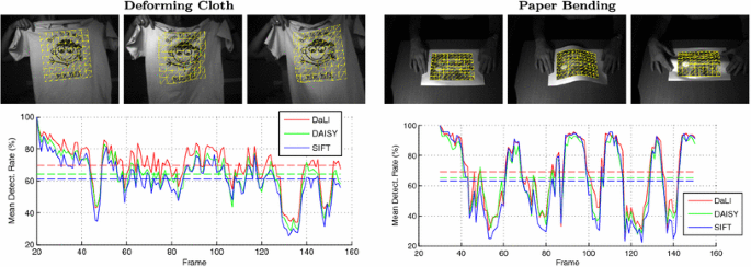
Mean detection accuracy on two real world videos from Moreno-Noguer and Fua (2013). In the top row we show three example frames from each video. In the bottom row we plot the accuracy for each frame for three descriptors: DaLI, DAISY and SIFT. Additionally the mean for each descriptor is displayed as a dashed line

References
Aflalo, Y., Bronstein, E. M., Bronstein, M. M., & Kimmel, R. (2011). Deformable shape retrieval by learning diffusion kernels. In In Proc. SSVM.
Aubry, M., Schlickewei, U., & Cremers, D. (2011). The wave kernel signature: A quantum mechanical approach to shape analysis. In Computer Vision Workshops (ICCV Workshops), 2011 IEEE International Conference on (pp. 1626–1633).
Bay, H., Tuytelaars, T., & Gool, L. V. (2006). SURF: Speeded up robust features. In European Conference on Computer Vision (pp. 404–417).
Belongie, S., Malik, J., & Puzicha, J. (2002). Shape matching and object recognition using shape contexts. IEEE Transactions Pattern Analysis and Machine Intelligence, 24(4), 509–522.
Berg, A., Berg, T., & Malik, J. (2005). Shape matching and object recognition using low distortion correspondences. In IEEE Conference on Computer Vision and Pattern Recognition (pp. 26–33).
Bronstein, A., Bronstein, M., Bruckstein, A., & Kimmel, R. (2007). Analysis of two-dimensional non-rigid shapes. International Journal of Computer Vision, 78(1), 67–88.
Bronstein, M., & Kokkinos, I. (2010). Scale-invariant heat kernel signatures for non-rigid shape recognition. In IEEE Conference on Computer Vision and Pattern Recognition (pp. 1704–1711).
Cai, H., Mikolajczyk, K., & Matas, J. (2011). Learning linear discriminant projections for dimensionality reduction of image descriptors. IEEE Transactions Pattern Analysis and Machine Intelligence, 33(2), 338–352.
Calonder, M., Lepetit, V., Ozuysa, M., Trzcinski, T., Strecha, C., & Fua, P. (2012). BRIEF: Computing a local binary descriptor very fast. IEEE Transactions Pattern Analysis and Machine Intelligence, 34(7), 1281–1298.
Chavel, I. (1984). Eigenvalues in Riemannian geometry. London: London Academic Press.
Cheng, H., Liu, Z., Zheng, N., & Yang, J. (2008). A deformable local image descriptor. In IEEE Conference on Computer Vision and Pattern Recognition.
Cho, M., Lee, J., & Lee, K. (2009). Feature correspondence and deformable object matching via agglomerative correspondence clustering. In International Conference on Computer Vision (pp. 1280–1287).
Fan, B., Wu, F., & Hu, Z. (2012). Rotationally invariant descriptors using intensity order pooling. IEEE Transactions Pattern Analysis and Machine Intelligence, 34(10), 2031–2045.
Gębal, K., Bærentzen, J. A., Aanæs, H., & Larsen, R. (2009). Shape analysis using the auto diffusion function. In Proceedings of the Symposium on Geometry Processing, SGP ’09 (pp. 1405–1413).
de Goes, F., Goldenstein, S., & Velho, L. (2008). A hierarchical segmentation of articulated bodies. In Proceedings of the Symposium on Geometry Processing, SGP ’08 (pp. 1349–1356).
Gupta, R., & Mittal, A. (2007). Illumination and Affine-Invariant Point Matching using an Ordinal Approach. In International Conference on Computer Vision.
Gupta, R., & Mittal, A. (2008). Smd: A locally stable monotonic change invariant feature descriptor. In European Conference on Computer Vision (pp. 265–277).
Gupta, R., Patil, H., & Mittal, A. (2010). Robust order-based methods for feature description. In IEEE Conference on Computer Vision and Pattern Recognition.
Heikkilä, M., Pietikäinen, M., & Schmid, C. (2009). Description of interest regions with local binary patterns. Pattern Recognition, 42(3), 425–436.
Ke, Y., & Sukthankar, R. (2004). PCA-SIFT: a more distinctive representation for local image descriptors. In IEEE Conference on Computer Vision and Pattern Recognition (pp. 506–513).
Kokkinos, I., Bronstein, M., & Yuille, A. (2012). Dense Scale Invariant Descriptors for Images and Surfaces. Research Report RR-7914, INRIA.
Kovnatsky, A., Bronstein, M., Bronstein, A., & Kimmel, R. (2011). Photometric heat kernel signatures. In International Conference on Scale Space and Variational Methods in Computer Vision (pp. 616–627).
Leordeanu, M., & Hebert, M. (2005). A spectral technique for correspondence problems using pairwise constraints. In International Conference on Computer Vision (pp. 1482–1489).
Lévy, B. (2006). Laplace-Beltrami Eigenfunctions: Towards an Algorithm that Understands Geometry. In IEEE International Conference on Shape Modeling and Applications - SMI 2006 (p. 13).
Ling, H., & Jacobs, D. (2005). Deformation invariant image matching. In International Conference on Computer Vision (pp. 1466–1473).
Ling, H., & Jacobs, D. (2007). Shape classification using the inner-distance. IEEE Transactions Pattern Analysis and Machine Intelligence, 29(2), 286–299.
Ling, H., Yang, X., & Latecki, L. (2010). Balancing deformability and discriminability for shape matching. In European Conference on Computer Vision.
Litman, R., & Bronstein, A. (2014). Learning spectral descriptors for deformable shape correspondence. Pattern Analysis and Machine Intelligence, IEEE Transactions on, 36(1), 171–180.
Lowe, D. (2004). Distinctive image features from scale-invariant keypoints. International Journal of Computer Vision, 60(2), 91–110.
Mikolajczyk, K., & Schmid, C. (2005). A performance evaluation of local descriptors. IEEE Transactions Pattern Analysis and Machine Intelligence, 10(27), 1615–1630.
Morel, J., & Yu, G. (2009). ASIFT: A new framework for fully affine invariant image comparison. SIAM Journal on Imaging Sciences, 2(2), 438–469.
Moreno-Noguer, F. (2011). Deformation and illumination invariant feature point descriptor. In IEEE Conference on Computer Vision and Pattern Recognition (pp. 1593–1600).
Moreno-Noguer, F., & Fua, P. (2013). Stochastic exploration of ambiguities for nonrigid shape recovery. Pattern Analysis and Machine Intelligence, IEEE Transactions on, 35(2), 463–475.
Philbin, J., Isard, M., Sivic, J., & Zisserman, A. (2010). Descriptor learning for efficient retrieval. In European Conference on Computer Vision (pp. 677–691).
Pinkall, U., & Polthier, K. (1993). Computing discrete minimal surfaces and their conjugates. Experimental Mathematics, 2(1), 15–36.
Raviv, D., Bronstein, M. M., Sochen, N., Bronstein, A. M., & Kimmel, R. (2011). Affine-invariant diffusion geometry for the analysis of deformable 3d shapes. In IEEE Conference on Computer Vision and Pattern Recognition.
Reuter, M., Wolter, F., & Peinecke, N. (2006). Laplace-beltrami spectra as ’shape-dna’ of surfaces and solids. Computer Aided Design, 38(4), 342–366.
Rustamov, R. (2007). Laplace-beltrami eigenfunctions for deformation invariant shape representation. In Eurographics Symposium on Geometry Processing (pp. 225–233).
Sanchez, J., Ostlund, J., Fua, P., & Moreno-Noguer, F. (2010). Simultaneous pose, correspondence and non-rigid shape. In IEEE Conference on Computer Vision and Pattern Recognition (pp. 1189–1196).
Serradell, E., Glowacki, P., Kybic, J., Moreno-Noguer, F., & Fua, P. (2012). Robust non-rigid registration of 2d and 3d graphs. In IEEE Conference on Computer Vision and Pattern Recognition.
Shi, L., Yu, Y., & Feng, N. B. W. W. (2006). A fast multigrid algorithm for mesh deformation. ACM SIGGRAPH, 25(3), 1108–1117.
Sochen, N., Kimmel, R., & Malladi, R. (1998). A general framework for low level vision. IEEE Transactions on Image Processing, 7(3), 310–318.
Strecha, C., Bronstein, A. M., Bronstein, M. M., & Fua, P. (2012). LDAHash: Improved matching with smaller descriptors. IEEE Transactions Pattern Analysis and Machine Intelligence, 34(1), 66–78.
Sun, J., Ovsjanikov, M., & Guibas, L. (2009). A concise and provably informative multi-scale signature based on heat diffusion. In Eurographics Symposium on Geometry Processing (pp. 1383–1392).
Tang, F., Lim, S.H., Chang, N., & Tao, H. (2009). A novel feature descriptor invariant to complex brightness changes. In IEEE Conference on Computer Vision and Pattern Recognition (pp. 2631–2638).
Tola, E., Lepetit, V., & Fua, P. (2010). Daisy: An efficient dense descriptor applied to wide-baseline stereo. IEEE Transactions Pattern Analysis and Machine Intelligence, 32(5), 815–830.
Torresani, L., Kolmogorov, V., & Rother, C. (2008). Feature correspondence via graph matching: Models and global optimization. In European Conference on Computer Vision (pp. 596–609).
Trulls, E., Kokkinos, I., Sanfeliu, A., & Moreno-Noguer, F. (2013). Dense segmentation-aware descriptors. In IEEE Conference on Computer Vision and Pattern Recognition.
Trulls, E., Tsogkas, S., Kokkinos, I., Sanfeliu, A., & Moreno-Noguer, F. (2014). Segmentation-aware deformable part models. In IEEE Conference on Computer Vision and Pattern Recognition.
Vaxman, A., Ben-Chen, M., & Gotsman, C. (2010). A multi-resolution approach to heat kernels on discrete surfaces. ACM SIGGRAPH, 29(4), 121.
Vedaldi, A., & Fulkerson, B. (2008). VLFeat: An open and portable library of computer vision algorithms. http://www.vlfeat.org/
Vedaldi, A., & Soatto, S. (2005). Features for recognition: Viewpoint invariance for non-planar scenes. In International Conference on Computer Vision (pp. 1474–1481).
Wang, Z., Fan, B., & Wu, F. (2011). Local intensity order pattern for feature description. In International Conference on Computer Vision (pp. 603–610).
Wesseling, P. (2004). An Introduction to multigrid methods. Chichester: Wiley.
Yanowitz, S., & Bruckstein, A. (1989). A new method for image segmentation. Computer Vision, Graphics, and Image Processing, 46(1), 82–95.
Yezzi, A. (1998). Modified curvature motion for image smoothing and enhancement. IEEE Transactions on Image Processing, 7(3), 345–352.
Acknowledgments
This work has been partially funded by the Spanish Ministry of Economy and Competitiveness under Projects ERA-Net Chistera project ViSen PCIN-2013-047 and PAU+ DPI2011-27510, and by the EU Project IntellAct FP7-ICT2009-6-269959.
Author information
Authors and Affiliations
Corresponding author
Additional information
Communicated by Ron Kimmel.
Rights and permissions
About this article

Cite this article
Simo-Serra, E., Torras, C. & Moreno-Noguer, F. DaLI: Deformation and Light Invariant Descriptor. Int J Comput Vis 115, 136–154 (2015). https://doi.org/10.1007/s11263-015-0805-1
Received:
Accepted:
Published:
Issue Date:
DOI: https://doi.org/10.1007/s11263-015-0805-1