Abstract
A meta-analysis and an experiment show that the degree of compression of the in-depth dimension of visual space relative to the frontal dimension increases quickly as a function of the distance between the stimulus and the observer at first, but the rate of change slows beyond 7 m from the observer, reaching an apparent asymptote of about 50 %. In addition, the compression of visual space is greater for monocular and reduced cue conditions. The pattern of compression of the in-depth dimension as a function of distance is similar to the ratio of in-depth to frontal visual angles of stimuli, but is not as extreme as this ratio would suggest, implying that observers are incapable of fully ignoring size information provided by cues to depth. Size and distance judgments may be described by an Affine transformation of physical space; however, the compression parameter in this model changes as a function of distance from the observer and other experimental conditions.
1 Does Visual Space Exist and is it a Single Entity?
When most people think of space, they think of physical space. The properties of physical space are objectively defined in terms of physical measuring devices like rulers and protractors. Many perceptual psychologists and philosophers are interested in another sort of space: visual space. Visual space concerns space as we consciously experience it, and it is studied through subjective measures, such as asking people to use numbers to estimate perceived distance. However, since we can’t directly observe conscious experience, visual space must be defined operationally in terms of the measures that we use. If the subjective measures were unrelated to visual experience, the whole field would be pretty boring, but most researchers, in our heart of hearts, believe that the judgments and estimates observers give are closely tied to their experience.
Visual space can differ dramatically from physical space under very ordinary conditions. This is problematic since research has shown that spatial abilities influence performance on a wide range of real-world tasks. For example, research has shown that mismatches between physical space and perception can adversely affect driving (Hiro 1997), flying (Roscoe 1985), railroad operation (Kong et al. 1995), sports performance (Shaffer et al. 2004), surgery (Reinhardt and Anthony 1996), and witness reliability (Moore 1907).
Philosophers and psychologists have suggested a wide variety of models to describe the geometry of visual space. For example, Thomas Reid (1764/1813), whose work inspired the current special issue, constructed a geometry of “visibles” based upon what the “eye alone can see” without taking into account cognition, inference, experience, or motion. He believed that the eye itself is incapable of depth perception; so, visual experience was akin to a projection on a sphere of arbitrary radius centered on the observer. Mathematically, this defines a spherical geometry, which has special properties such as that parallel lines can not exist in the space and that the sum of the angles of a triangle are always >180°.
However, Reid’s model for visual space is only one of many that have been proposed. Other scholars have suggested that visual space is best described by a Euclidean geometry (Fry 1950; Gibson 1950, 1959, 1966; Kant 1781/1929), a hyperbolic geometry (Blank 1953, 1957, 1958, 1959; Heller 1997; Indow 1967, 1974, 1990, 1995; Luneburg 1947, 1948, 1950), a Lie transformation group (Hoffman 1966; Hoffman and Dodwell 1985), and a Cayley-Klein geometry (Drösler 1979, 1988, 1995). Many others have described visual space in terms of various transformations of physical space (e.g., Baird and Wagner 1991; Foley et al. 2004; Gilinsky 1951; Hatfield 2003, 2009, 2012; Wagner 1985, 2006, 2012).
While the existence of so many competing models for visual space might simply be evidence of a healthy academic debate, a greater challenge for the concept of visual space comes from the diversity in the metric judgments observers produce. For example, in a meta-analysis of 413 data sets in which observers directly estimated the metric properties of visual space (such as distance or angle), Wagner (2008) found estimates varied significantly as a function of observer age, cue conditions (full vs. reduced cue), setting (laboratory vs. outdoors), judgment method, presence of a standard, stimulus orientation (frontal vs. in-depth), stimulus range, and stimulus type (direct perception vs. memory or cognitive maps). Cognitive-mapping-based estimates also varied significantly as a function of days of acquisitions and environmental scale. In a meta-analysis of 125 data sets concerning size-constancy judgments, Wagner (2012) found that size judgments varied significantly as a function of instructions (objective vs. apparent, projective, or perspective), cue conditions (full vs. reduced cue), stimulus orientation (frontal vs. in-depth), and observer age.
Such diversity in estimates flies in the face of the simple idea of visual space being a single, unchanging, unitary image in our mind. The search for a single space that might be labeled “the geometry of visual space” seems hopeless. There are two common responses in today’s spatial literature to this challenge: recharacterize some of the data as being non-perceptual to hold onto the idea of a single visual space or abandon the whole concept of visual space altogether.
The first tendency is often seen in response to instruction effects in size-constancy judgments. There is a general tendency for objective and perspective instructions to produce over-constancy (the sizes of distant stimuli are overestimated), apparent instructions produce constancy on the average (or slight under-constancy), and projective instructions produce strong under-constancy (the sizes of distant stimuli are underestimated) (Wagner 2012). Many early researchers believed that common reports of over-constancy were theoretically suspect since they believed that spatial judgments represented a compromise between physically accurate judgment and the projective image on the retina (Brunswik 1929, 1933, 1956; Teghtsoonian 1974). Since over-constancy falls outside of this range, it should not be possible—the achieved cannot exceed the potentially achievable (Koffka 1935). More recent researchers have expressed this objection in the language of cognitive psychology. They argue that there really is only one visual space in our perceptual experience that is best revealed by apparent size instructions, while other instructions, particularly those resulting in over-constancy, involve a cognitive overlay on perception in which observers supplement perception with their knowledge about how distance affects size (Gogel 1990, 1993, 1998; Granrud 2009, 2012; Hatfield 2003, 2009, 2012; Predebon 1990, 1992). In effect, some judgments reflect the real visual space, while others do not reflect visual space but are useful responses to it.
In our opinion, there is no need to demote certain types of judgments in order to maintain a simple, unitary view of visual space. It is better to embrace the idea that visual space is a living, malleable entity whose geometry changes with experimental conditions and shifts in observer attitude. Wagner (2012) points out that there is no reason to prefer apparent size judgments as best reflecting visual space since good arguments can be made that (1) projective instructions more nearly match the result of “bracketing out” cognitive influences, that (2) apparent instructions must take into account cognitive factors to achieve constancy, and that (3) objective instructions more nearly match the “natural attitude” of adult observers under ordinary circumstances. Wagner also points out that unless all of the cognitive operations take place at a conscious level (and no one argues that), there is no way to objectively determine the degree to which judgments reflect perception as opposed to cognition for any instruction type, since the unconscious mind is a black box whose contents can never be confirmed. In the end, what we are left with are variations in observer judgments. Since subjective experience cannot be directly observed, we must operationally define visual space in terms of the judgments observers generate. If one accepts that visual space must be defined in terms of the judgments observers make, then there is no basis for accepting some judgments as reflecting the real visual space while others are rejected. One must accept that the character and form of visual space changes as a function of stimulus conditions and observer attitudes; that is, visual space is more than one thing.
Still, the idea that there is a single “picture in our head” is phenomenologically compelling. Yet, even if we only have one image of the world, humans are capable of organizing their perceptual experiences in multiple ways. The same image can result in more than one Gestalt (Köhler 1926). Even if there is only one image of the world in our heads, this simply provides the coordinates for our experience. In geometry, one set of coordinates can result in an infinite number of geometries by simply changing the metric functions that define distance and other metric properties. Thus, a single image in the head can support multiple meanings for size and distance. Once again, visual space need not be only one thing.
A greater challenge to the concept of visual space comes from another direction. A number of researchers have questioned the usefulness of the very concept of visual space and even questioned its existence (e.g., Smeets et al. 2009). These researchers point to inconsistencies in spatial judgments and unusual contextual effects to make their case. For example, Luria et al. (1967) and Thorndyke (1981) found that intervals containing intervening objects are seen as longer than empty intervals. Norman et al. (2000) found that lengths oriented along the curved dimension of a cylinder were perceived to be longer than the same lengths along a flat surface. From this, they conclude that perceived length critically depends on the structure of the object in which the length occurs. Similarly, Bian and Andersen (2011) found that exocentric distance judgments changed when judged along a ceiling compared to along the ground. Both Schoumans et al. (2002) and Cuijpers et al. (2001) found that the presence of reference stimuli or reference frames altered perceived orientation and angle. Doumen et al. (2005) found inconsistencies between exocentric pointing, collinearity, and parallelity tasks, leading them to conclude that the structure of visual space depends on the task. Finally, Smeets et al. (2009) found that 2-D visual illusions produce judgments incompatible with any well-behaved geometry. From this, they conclude that the concept of visual space is not particularly useful.
So, does this recent work demand that we abandon the concept of visual space? We don’t think so; but it does strongly challenge the belief that visual space is one, unchanging entity with a geometrically simple structure. We believe that the main lesson we can derive from the last 100 years of research, both old and new, is that visual space is strongly influenced by context, including things like judgment methods, instructions, and stimulus conditions. So, we find it odd, when people say that we should abandon the concept of visual space just because there are contextual effects. The goal of our studies should be to specify exactly how metric estimates of visual space change in response to these contextual variables. Mathematically, we should incorporate these other factors into our metric equations to predict perceptual judgments.
Does visual geometry exist under all circumstances? Well, ask yourself if you have ever had an occasion in which you looked at the world and your visual experience ceased to be spatial? Don’t you always have a sense that one thing is to the left of another, one thing is above another, or one thing is closer than another? Visual space always exists but the exact geometry changes with circumstances. The possible exception to this is in cognitive maps, whose fragmented and hole-ridden structures may not even satisfy the assumptions of a Riemannian manifold, since a Riemannian manifold assumes that adjacent points in a space smoothly connect to one another.
Having said this, visual space need not be simple, and it certainly does not need to be Euclidean. In fact the judgments that observers produce often violate some of the most basic axioms of most known geometries. For example, Wagner (2006) showed that visual space violates virtually every axiom of a geometry of constant curvature (which includes both Euclidean geometry and Reid’s spherical geometry), and that spatial judgment are not always even consistent with three of the four axioms of a metric space—one of the most general geometric structures. So, while our phenomenal experience tells us that visual space exists, the judgments that observers produce point to a complex space that varies along with context and observer attitude.
2 Affine Transformations and the Anisotropy of Visual Space
While models for visual space come and go, the empirical data on which these models are based are more enduring. One common finding is that the in-depth of dimension of visual space is perceptually compressed (with a few exceptions) compared to the frontal dimensions. Some researchers use the term anisotropy to label this phenomenon. (This term as used in physics usually refers to variations in the properties of a space as a function of direction from the observer, but it is also used to indicate variations in the properties of a space along different axes in a more general sense. The second sense of the term applies here).
For example, Wagner (1982, 1985) pounded stakes randomly in a large, flat, grassy field, and asked observers to judge distances between pairs of stakes and angles formed by stake triplets using four different psychophysical methods (magnitude estimation, category estimation, perceptual matching, and mapping) with apparent size instructions. The data revealed that stimulus orientation affected judgments in the same way for all judgment methods. For stimuli spanning the same physical distance, those receding away from the observer in depth were seen to be about half as large on the average as those oriented frontally with respect to the observer. Angle judgments showed an analogous pattern. For angles of the same physical size, those whose open ends faced either toward or away from the observer expanded perceptually, while those whose open ends face to the right or left (the observer looks across the legs of the angle) perceptually contract. In other words, the judged angle is larger than the physical angle for angles that face toward or away from the observer, while the judged angle is smaller than the physical angle for angles facing to the left or right relative to the observer.
Both sets of data are consistent with a general compression of the in-depth dimension of visual space relative to the frontal dimension. The compression makes in-depth oriented stimuli seem shorter than physically equal stimuli oriented frontally with respect to the observer. The legs of angles facing directly toward or away from the observer are squeezed apart as by the compression of the in-depth dimension, while the legs of angles facing off to either side are squeezed together by this compression.
Wagner (1982, 1985) tested 12 candidate metrics to fit these data and found that two of them fit judgments much better than the others. The first was called the Affine Contraction model. In this model, the observer is located at the origin of a Euclidean plane with the x-axis corresponding to the left–right frontal dimension and the y-axis corresponds to the observer’s in-depth dimension. According to the model, the frontal dimension is accurately perceived, while the in-depth dimension is perceptually compressed. After the transformation, the space is still assumed to be Euclidean. Based upon this model, the following formula describes the relationship between perceived distance, s′, and the physical coordinates of the two end points (x 1 ,y 1) and (x 2,y 2):
where c reflects the degree of compression of the in-depth dimension of visual space.
For distance judgments, Wagner found that all three judgment methods displayed very similar amounts of compression, averaging c = 0.45. In other words, the same physical stimulus oriented in-depth seemed to be less than half as large as when that stimulus is oriented frontally. Using a formula from Riemannian geometry, the same model can be applied to the angle data as well, and this data yielded a similar degree of compression across all methods that corresponded closely to the value of c obtained with distance judgments. For angle judgments on the average c = 0.48.
One aspect of the Affine Contraction model seemed unrealistic. Stimuli parallel to an observer’s line of sight should all experience the same degree of compression no matter where they are in the visual field, even though such stimuli far to the left or right of the line of sight would actually be seen as largely frontally oriented if the observer simply looked in their direction. So, any eye, head, or body reorientation should lead to a change in perceived size, which seemed unlikely. To correct for this problem, Wagner considered a second model that is a variation on the Affine Contraction model, which he called the Vector Contraction model. In this model, distances in visual space can be thought of as vectors that can be decomposed into frontal (V1) and in-depth (V2) components and the in-depth component is compressed in visual space by a factor c. The Vector Contraction model produced similar degrees of compression (on the average c = 0.45 for distance judgments and c = 0.48 for the angle judgments once again) and fit the data slightly better than the Affine Contraction model.
Wagner and Feldman (1989) extended this work to three dimensions and under both light and dark viewing conditions. (See Wagner 2006, for details.) Under full-cue conditions, the compression parameter averaged c = 0.52 for distance judgments and c = 0.62 for angle judgments. The degree of compression of the in-depth dimension was more extreme under reduced cue conditions, as c = 0.35 for distance judgments and c = 0.32 for angle judgments.
3 Factors that Affect the Degree of Anisotropy
In subsequent years, many other researchers have explored the anisotropy of visual space or suggested that Affine transformations are useful in describing visual space. For example, Toye (1986) asked observers to judge distances between 13 stimuli randomly placed in a 21 m diameter circular patch of a flat, grassy field using objective instructions over two sessions. Some of his observers made both sets of judgments from the same position each time, while others moved 90° along the edge of the circle; so, for their second set of judgments, any distances that were oriented in-depth relative to the observer during the first set of judgments were now frontally oriented and frontally oriented stimuli were now see in-depth. Among the four observers who shifted positions, Toye found the average ratio of in-depth to frontal judgments for the same stimuli (what I call the compression parameter) was c = 0.85. Thus, while Toye also found compression of the in-depth dimension of visual space relative to the frontal dimension, it was not as extreme as that of Wagner (1982, 1985) or Wagner and Feldman (1989). As we shall see repeatedly, nearer stimuli result in less anisotropy. Toye’s stimuli were nearer to the observers than Wagner’s (1982, 1985).
Similarly, Haber et al. (1993) asked observers to judge distances between objects in an information rich, indoor office environment using objective instructions. They also found that in-depth oriented distances were estimated to be shorter than physically equivalent distances oriented frontally. The degree of compression appears to be less extreme than Wagner found, although the data is not formatted in a way to make it possible to state a precise value for c. Once again, information-rich environments with relatively nearer stimuli seem to lead to less anisotropy.
Loomis et al. (1992) confirmed that distance to stimuli influences the degree of compression of the in-depth dimension of visual space. They had observers adjust the length of an in-depth oriented comparison until it appeared equal to frontally oriented standards using objective instructions in two experiments. The standards ranged between 4 to 12 m from the observer. In the first experiment, they found compression parameters ranging from c = 0.73 for the nearest standard to c = 0.46 for the most distant one. In the second experiment, compression parameters ranged from c = 0.73 for the nearest standard to c = 0.60 for the most distant. Thus, in both experiments the degree of compression of the in-depth dimension of visual space appears to grow with increasing distance from the observer.
Hecht et al. (1999) reached a similar conclusion based on angle judgments. They asked observers to judge the apparent size of 6 angles formed by building walls (ranging from 108° to 161.5°), three of the angles faced toward the observer and three faced away from the observer. In every case, the angles seem to perceptually expand, just as Wagner (1982, 1985) found. In a separate study, observers judged the size of a 90° angle facing toward the observers from three different distances away from the angles—ranging from 1.5 to 23.4 m. Observers overestimated the size of the angle at all three distance, but overestimation increased with increasing distance from the observer. This result is consistent with greater compression of the in-depth dimension of visual space as distance increases.
Loomis et al. (2002) not only showed that compression of the in-depth dimension changes with distance, but that under certain circumstances with very near stimuli, the in-depth dimension of visual space can actually expand relative to the frontal dimension. They preformed two experiments. In the first, observers adjusted an in-depth interval until it appeared to equal a frontal stimulus using both monocular and binocular conditions. For near stimuli (20–50 cm from the observer) the degree of compression averaged c = 0.90 under monocular conditions, but was actually greater than one (c = 1.03) under binocular conditions, indicating that the in-depth dimension was actually expanded relative to the frontal dimension for these very near stimuli. For more distant stimuli (ranging from 2 to 4 m from the observer), visual space showed compression for both monocular (c = 0.86 at 2 m and c = 0.78 at 4 m) and binocular (c = 0.91 at 2 m and c = 0.83 at 4 m). In the second experiment, they asked observers to estimate the depth to frontal extent of various depth and frontal interval combinations located at different distances away from the observer. Under monocular, conditions the compression parameter was c = 0.80 for stimuli 1 m away and c = 0.67 for stimuli 1.5 or 2 m away. For binocular conditions, the compression parameter ranged from c = 0.87 for stimuli 1 m away to c = 0.82 for stimuli for those 1.5 or 2 m away.
Tittle et al. (1995) confirmed that the in-depth dimension of visual space is expanded relative to the frontal dimension (c > 1.0) for stimuli nearer than 1 m from the observer and compressed for stimuli greater than 1 m away (c < 1.0). They presented stereoscopic and motion-based depth cues using a random-dot stereogram while observers sat either 0.75 or 1.75 m from the screen. In their first experiment, they asked observers to adjust display parameters until a depth interval appeared to match the frontal interval. Their results were consistent with an expansion of the in-depth dimension relative to the frontal dimension for 0.75 m away from the observer and a compression of the in-depth dimension when observers sat 1.75 m away. In the second experiment, they asked observers to adjust an angle facing toward them until it appeared to equal 90°. For stimuli less than 1 m away, observers tended to make the angle too big, which means that observers see the angle as smaller than it is—a result consistent with an expansion of the in-depth dimension. On the other hand, stimuli more than 1 m away led observers to make the angle too small, which means the observers see the angles as being larger that it is physically—a result that is consistent with a compression of the in-depth dimension of visual space relative to the frontal dimension. Thus, in both experiments the in-depth dimension of visual space expands for very near stimuli and is compressed for more distant ones.
Cuijpers et al. (2000) used a different strategy to show the effects of distance on anisotropy. They asked observers to adjust pointers so that it seemed to point at targets ranging from 1 to 5 m from the observer. If the pointer direction was closer to the frontal plane than the true direction, this would indicate that visual space is perceptually compressed in the in-depth dimension, while pointers that deviate the other way from the true direction would indicate an expansion of the in-depth dimension relative to the frontal dimension. Once again, they found an expansion in the in-depth dimension for stimuli very near the observer and compression in the in-depth dimension for stimuli located further from the observer.
Li et al. (2013) asked observers to match either in-depth or frontal extents ranging from 1.5 to 7 m from the observer by either blind walking or adjusting a comparison extent. For both judgment methods, in-depth oriented extents were judged to be shorter than frontally oriented ones and the degree of underestimation increased with distance from the observer. The compression parameter declined from approximately c = 0.86 at 1.5 m to c = 0.78 at 7 m.
Besides Loomis et al. (2002), several other studies have looked at the effects of stereopsis on depth compression. For example, Sipes (1997) confirmed that visual space is compressed in the in-depth dimension and that the degree of compression increased along with viewing distance. Sipes theorized that the compression is reduced at near distances because stereoscopic cues are more effective near the observer. Sipes used a series of mirrors to increase interocular distance and thus increase the effectiveness of stereoscopic cues. Under these hyperstereoscopic conditions, Sipes found that compression of the in-depth dimension was greatly reduced.
Similarly, Loomis and Philbeck (1999) asked observers to judge the ratio of depth to width for two different L-shaped configurations in which one rod was oriented in-depth and another was oriented frontally. The L-shaped configurations were either near the observer (3.9–6.5 m away) or further away (11.7–19.5 m). The more distant stimuli were also larger in size to match the visual angles of the nearer stimuli and observers stood on a staircase to match the optical slant (or angle of regard) of the near stimuli. They found that the observers’ judgments did not differ between the two configurations for monocular viewing (although the compression parameter decreased as a function of distance within each configuration), but there was significantly more compression of the in-depth dimension for distant stimuli than for near stimuli under binocular conditions. The fact that judgments were nearly the same for the two configurations under monocular conditions led the authors to conclude that optical slant is a key variable in determining the anisotropy of visual space when binocular cues to depth are missing; however, given the set up of the experiment, one could as easily conclude that the visual angle of a stimulus is a key factor in determining anisotropy since visual angle varied along with optical slant in their experiment.
Wu et al. (2008) asked observers to match a in-depth oriented comparison (ranging from 5 to 7 m from the observer) to a frontally oriented standard placed either far away from the observer, near the observer, or adjacent to the comparison stimulus. Judgments were made both monocularly and binocularly under both full-cue and reduced-cue conditions. Wu et al. found compression of the in-depth dimension for all conditions. The degree of compression (under full-cue conditions) was greater under monocular conditions (c = 0.61) than it was under binocular conditions (c = 0.72). Compression of the in-depth dimension (under full-cue conditions with monocular viewing) increased with increasing distance from the observer from c = 0.63 at 5 m to c = 0.58 at 7 m. Compression of the in-depth dimension of visual space (binocular viewing) was greater under reduced cue conditions (c = 0.47) than full-cue conditions (c = 0.72). They also found that the degree of compression was smaller when the standard was near the observer than in the other two conditions.
Finally, Bingham and Lind (2008) have found that anisotropy can be greatly attenuated if observers are allowed to move and see the stimulus arrangement from more than one perspective. They found that stationary observers or those whose perspective changes less than 45° show anisotropy, while those who move either continuously or discretely so that their perspective changes 45° or more show little anisotropy.
In summary, the degree of compression of the in-depth dimension of visual space is not constant, but varies as a function of a number of factors. First and foremost, distance affects anisotropy. Very near the observer, the in-depth dimension of visual space actually expands relative to the frontal dimension. Beyond about 1 m from the observer the in-depth dimension is generally compressed relative to the frontal dimension and this compression increases with distance from the observer. The compression is greater under reduced-cue conditions than full-cue conditions, when plenty of cues to depth are available. Stereopsis, in particular, affects the degree of anisotropy. When stereopsis is present (or magnified), the compression of the in-depth is attenuated. Increased information about layout resulting from motion and changing perspective also attenuates the effect.
4 A Meta-analysis of the Affect of Distance on Anisotropy
Although many researchers have explored the anisotropy of visual space and tested whether Affine transformations can be used to model it, relatively few present data in a way that make it possible to calculate the compression parameter, c. We have preformed a small meta-analysis of articles for which this possible. For each of these studies, we calculated the value of c based upon data contained in figures found in the article. We calculated a value of c separately for each distance from stimulus to the observer reported. In a few cases, stimuli had a randomly selected range of distances; in this case, we recorded the average distance from the observer to the stimuli. In addition, to distance and compression parameters, we also recorded whether objective or apparent instructions were used, whether judgments were made binocularly or monocularly, and whether judgments were made under full-cue or reduced-cue conditions. If the study used more than one standard, we calculated the compression parameters for each standard and recorded the average value of c.
One older study presented a special challenge. Although Baird and Biersdorf (1967) did ask observers to judge the objective size of both frontally and in-depth oriented stimuli at a variety of distance, the actual set of distances from the observer that they used varied between frontal and in-depth judgments. So, we used interpolation on the in-depth judgments in order to estimate what those judgments would be if at the same distances away from the observer used for frontal judgments.
Following this method, we recorded 59 cases across 10 studies. Figure 1 shows the results of this meta-analysis. The figure shows the compression parameter as a function of the distance stimuli were from the observer. Filled symbols represent judgments under full-cue, binocular conditions, where diamonds indicate the use of objective size instructions (34 cases) and squares represent the use of apparent size instructions (5 cases). Open symbols represent judgments under full-cue, monocular conditions, where diamonds indicate the use of objective instructions (12 cases) and squares represent the use of apparent size instructions (3 cases). The “x” symbols represent judgments collected under reduced-cue conditions (5 cases). All of the reduced-cue judgments were done binocularly with apparent size instructions.

Meta-analysis of the compression parameter as a function of the distance stimuli were from the observer. Filled symbols represent judgments under full-cue, binocular conditions, where diamonds indicate the use of objective size instructions and squares represent the use of apparent size instructions. Open symbols represent judgments under full-cue, monocular conditions, where diamonds indicate the use of objective instructions and squares represent the use of apparent size instructions. The “x” symbols represent judgments collected under reduced-cue conditions
There are a number of observations one can make based upon this figure. First of all, it is apparent that the degree of compression of the in-depth dimension of visual space relative to the frontal dimension becomes more pronounced as distance from the observer increases. Under binocular conditions, stimuli very near the observer actually show an expansion of the in-depth dimension of visual space (c > 1.0), but the compression parameter rapidly declines until about 7 m from the observer. For even greater distances, it appears the compression parameter approaches an asymptote at a little below c = 0.5. Monocular judgments appear to produce slightly smaller compression parameters than binocular judgments. Reduced-cue conditions produce markedly smaller compression parameters than full-cue conditions.
The vast majority of the cases used objective instructions, and there is a tendency for objective instructions to be employed most often for near stimuli, while apparent instructions were used for more distant stimuli. With this cautionary note in mind, it is interesting to note how little effect instructions had on the overall trends. This is odd, since instructions have a dramatic affect on size judgments themselves. Objective instructions often produce over-constancy for frontally oriented stimuli and under-constancy for flat stimuli. Apparent instructions typically produce slight under-constancy for frontal stimuli and stronger under-constancy for flat stimuli. Yet, despite these strong effects of instructions on size judgments, the ratio of in-depth to frontal judgments appears to be largely unaffected by instruction type. Similarly, Wagner (1982, 1985) and others have shown that different judgment methods result in similar degrees of compression in the in-depth dimension (with the possible exception of blind walking). Once again, the judgment method one employs has significant effects on judgments of size and distance (Wagner 2008), while c, the ratio of in-depth to frontal judgments, is largely unaffected by judgment method. In addition, Wagner (1982, 1985) and Wagner and Feldman (1989) show that the compression parameters derived from angle judgments are consistent with those from distance judgments. Thus, it is possible that the pattern of anisotropy found in Fig. 1 may reflect a fact about visual space that rises above methodological concerns.
One challenge to this conclusion arises from Thouless’s (1931) early work on space perception. Thouless asked observers to make size judgments using what we would today call projective instructions under full-cue conditions (although the depth cues were not particularly good) of a series of in-depth oriented standards ranging between 0.545 to 1.635 m from the observer. He did this by asking observers to select among a set of ellipses and rectangles the comparison which best matched the standard. He found that the in-depth dimension was perceptually smaller than the frontal dimension for all stimuli, and that the difference between the in-depth and frontal judgments increased with distance from the observer. Thus, Thouless anticipated the data presented in Fig. 1; however, the degree of compression in the in-depth dimension that Thouless discovered was much more extreme than that presented in Fig. 1. Based on four observers, the compression parameters varied between c = 0.79 for 0.545 m distant stimulus to c = 0.49 for the stimulus 1.645 m away. If Thouless’s data was correct, it would appear that projective instructions are associated with much greater compression in the in-depth dimension than either objective or apparent size instructions.
In addition, the conclusion that the compression parameter reaches an asymptote at c = 0.5 is provisional and unlikely to be strictly true. It might be better to say that the rate of change in the compression parameter increasingly slows as distance grows beyond 7 m; however, at extreme distances it might be less than c = 0.5. The reason why this conclusion is so tentative is that there is little empirical data for size judgments at very large distances from the observer and little or no data available to calculate the compression parameter at these extreme distances. One rare exception was Flückiger (1991) who asked observers to judge the distance to boats on Lake Leman ranging between 0.75 and 5.6 km away from the observer. Cutting (2003) calculated the exponent for distance estimates as being about 0.4, which is much less than the average exponent of 1.02 that Wagner (2008) found in his meta-analysis of 263 perceptual distance estimation exponents. Although Flückiger’s data does not directly assess the anisotropy of visual space, it does suggest that the compression of visual space at extreme distances from the observer may be very large.
5 An Empirical Confirmation of the Meta-analysis
Figure 1 displays a remarkably clear and consistent pattern (particularly for full-cue binocular conditions) despite being based upon the work of disparate researchers using varying methodologies. To confirm the results of the meta-analysis, we decided to do a simple experiment to determine the values of the compression parameter as a function of distance from the observer. The experiment asks observers to judge the size of both frontally and in-depth oriented stimuli at seven distances from the observer ranging from 1 to 20 m away. Although it has a simple design, it does have the virtue of collecting judgments for stimuli across a greater number of distances and across a greater range of distances than previous work.
As we mentioned earlier, one of the main lessons of the last 100 years of research on space perception is that spatial judgments and visual space itself changes with context. So, any statements about spatial judgments are always in reference to a specific set of instructions and stimulus conditions. So, to be clear, this experiment involves binocular judgments under full-cue conditions. In addition, to further differentiate it from Baird and Biersdorf (1967), which is most similar to our study in design, we use instructions that emphasize that observers should judge apparent size and not objective size.
5.1 Method
5.1.1 Participants
Thirty-nine undergraduate students (13 men, 26 women) of Wagner College participated in the experiment. Participation in the experiment was voluntary, although the majority of participants did receive partial course credit toward their Introduction to Psychology grade. The participants were all within the age range of 18–22 years and had either normal or corrected vision. The experiment was approved by the college’s Human Experimentation Review Board, and in accord with its policies, all participants gave their informed consent before participating in this study. Participants were allowed to withdraw from the study at any time, but none did.
5.1.2 Materials and Experimental Layout
The study took place on an outdoor patio on the first floor of a building at Wagner College. Durable, all-weather tape, with a width of 4.78 cm, was used to make two rows of standard line-segment stimuli and to mark the origin line behind which the participants stood while making their judgments. Half of the line segments were oriented frontally, that is perpendicular to the participant’s line of sight (in the frontal plane), while the other half were oriented in-depth, that is aligned parallel to the observer’s line of sight (along the median plane). In each row, there were seven line segments laid out one behind the other along the participant’s line of sight. The centers of each line segment were 1, 3, 5, 7, 10, 15, and 20 m from the origin line on the ground in front of the participant. All of the line segments were 80 cm long and painted bright green to contrast with the patio surface. In the first row, the orientation of each line segment was randomly selected. The second row mirrored the layout of the first row; however, a line segment at a given distance that was oriented frontally in the first row was oriented in-depth in the second row, and any line segment at a given distance that was oriented in-depth in the first row was oriented frontally in the second. The unmarked backside of an adjustable tape measure served as an adjustable comparison for participants to make their judgments.
5.1.3 Procedure
Each of the 39 participants performed the experiment individually. The researcher measured the heights of the participants up to their eyes and recorded the measurements. The researcher then read the instructions to the participants. The participants were asked to stand behind the “origin” line and make judgments of the apparent size, rather than the objective size, of each line segment using an adjustable tape measure that was flipped over so that they could not see the numerical values of their measurements. For each line segment, the participants had to make two judgments; one with the measuring tape starting at 0 cm and the other with the measuring tape starting at greater than 80 cm. The participants made their judgments one row at a time, starting with the row to their left. Some participants (N = 20) started with the line segment nearest to them and worked their way to the farthest line segment, and the other participants (N = 19) started with the line segment farthest from them and worked their way to the nearest line segment. The researcher recorded each measurement in a book so that the participant could not see the recorded measurements. The researcher emphasized that the judgments needed to be of the apparent length of each line, rather than the objective length of each line. The exact instructions were:
You see two rows of seven lines in front of you at different distances away. Although these lines may be physically the same length, they might or might not appear or “look” that size subjectively. For each of the lines, I would like you to adjust the tape measure until it matches the apparent length of each line, excluding the box on the end. For each line I need you to do two adjustments, one where the tape is initially short and must be adjusted outward and one where the tape is initially long and must be adjusted inward. In between each adjustment, I will take the tape measure from you and record your estimate. Please don’t turn the tape measure over to see the numbers, since we want you to rely on your subjective impressions, not the numbers on the back. Start with the near (for half the participants) [or far (for half the participants)] line in the first row in front of you and then proceed to the next line. After you have estimated the apparent length of all lines in the first row, we will have you stand in front of the second row and go through the process again. Remember, we don’t want you to report the actual physical length of each line, but we want you to tell us how long each line looks or appears.
After completing their estimates, participants were thanked and debriefed about the purpose the experiment.
5.2 Results
This experiment examined judgments of the apparent lengths of line segments as a function of distance to each line segment and the orientation of each line segment. The dependent variable was the apparent length judgments made by the participants, and the three independent variables were the distance from the participant to each line segment (which we will call distance), the orientation of the line segments (which we will call orientation), and whether the judgment involved an ascending or descending judgment (which we will call trial type). To test the effects of these independent variables on judgments of apparent lengths a three-way repeated-measures Analysis of Variance was performed.
Close examination of the data revealed that two of the 39 observers generated essentially random data that varied wildly from trial to trial and showed no discernable pattern in judgments as a function of distance. The experimenter also noted that these two observers did not appear to be seriously engaged in the task. These two observers were eliminated from the analysis, leaving the judgments of 37 observers in the data set.
There was a significant main effect for orientation, F(1,36) = 26.39, p < .001, η2 = 0.42, on the apparent length judgments. On the average, the estimated apparent size for in-depth oriented stimuli (M = 21.76, SE = 2.57) was much smaller (and less variable) than that of frontally oriented stimuli (M = 28.15, SE = 3.35). Distance to the stimulus also had a significant main effect, F(6,216) = 103.96, p < .001, η2 = 0.74, on the judgments of apparent length. Although there was a significant effect of trial type, F(1,36) = 4.71, p = .037, η2 = 0.12, the different trials had no significant interaction with orientation and distance. Although the effect of trial type was significant, it was very small. The mean of all judgments made with ascending trials (M = 24.48) was almost the same as the mean of all judgments made with descending trials (M = 25.42).
There was a significant interaction between orientation and distance, F(6,216) = 9.36, p < .001, η2 = 0.21. Figure 2 shows mean apparent size judgments as a function of both distance from the observer and stimulus orientation. The mean apparent size judgments for each orientation showed that the line segments oriented in-depth were perceived as shorter than those oriented frontally after the first measurement at 1 m, that there was a steady decline in apparent length as the distance away from the observer increased, and that the decline is swifter for in-depth oriented stimuli than for frontally oriented ones (see Fig. 2). Thus, under these instructions that emphasized making judgments based upon apparent size, both frontal and in-depth oriented stimuli showed strong under constancy, with greater under constancy for the in-depth oriented stimuli. This contrasts with Baird and Biersdorf (1967) who found over-constancy for frontal stimuli and under-constancy for in-depth oriented stimuli based upon objective size instructions.

Mean apparent size judgments as a function of both distance from the observer and stimulus orientation. Squares represent mean judgments for frontal stimuli and diamonds represent mean judgments for in-depth oriented stimuli. Dashed lines represent the best fitting curves based on the transformation theory for size judgment for each data set
To calculate the compression parameter, c, we divided the mean apparent size judgments for in-depth oriented stimuli by the mean size judgments for frontally oriented stimuli at each distance from the observer. Figure 3 shows how the compression parameter changes as a function of distance from the observer in this experiment. The resulting pattern is very similar to that seen in the meta-analysis in Fig. 1. As in the meta-analysis, the compression parameter is larger than one for very near stimuli. It rapidly declines in size as a function of distance until about 7 m from the observer where the decline is less rapid. Once again, the compression parameter appears to reach an asymptote at about c = 0.5 for the most distant stimuli.

Compression parameter (the mean in-depth judgment divided by the mean frontal size judgment) as a function of distance away from the observer in the experiment
We should also note one other feature of the data. Although the averages show strong under-constancy for both frontally oriented and in-depth oriented stimuli, careful examination of the data for individual observers showed that a number of individuals did not follow this pattern. For estimates of frontally oriented stimuli, the data for 3 of the 37 observers displayed near constancy (estimated size for the most distant stimulus was within 5 % of the estimate for the nearest stimulus) and the data for three others showed over-constancy (size estimates for the most distant stimulus were more than 5 % greater than those for the nearest stimulus). Wagner (2012) suggested that apparent size instructions have historically led to constancy on the average because different observers interpret these instructions to mean different things. Some may interpret apparent size instructions to mean something akin to objective size, others interpret them as requiring projective size judgments, and others may interpret them as something in-between these extremes. Even in the current experiment where our instructions made it clear that we were not looking for objective size, the over-constancy shown by some observers may mean that they judged objective size despite our efforts.
6 Modeling Data from the Experiment
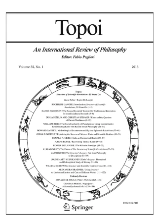
Wagner (2006) developed a mathematical model (which is a generalization of Baird and Wagner (1991) and of the Size-Distance Invariance Hypothesis) called the Transformation Theory for Size Judgment to model size constancy data. The key idea is that some information can be lost when visual information hits the retina. The retina only knows how much of the visual field an object takes up, what perceptual psychologists call the visual angle. Figure 4 shows a schematic displaying the visual angle (θ), target size (s), distance from the observer to the target (d), orientation of the target (ϕ), and height of the observer (h) in a typical size constancy experiment. The size of three-dimensional object represented in the figure is transformed into a visual angle with the following equation:

Schematic of the visual angle θ of a stimulus striking an idealized observer of height h viewing a target of size s at orientation ϕ located at distance d away from him/her. From Baird and Wagner (1991). Copyright 1991 by the American Psychological Association. Reprinted by permission
Note that this first transformation is a physical and takes place without error.
However, we experience objects three-dimensionally; so, the visual system must perform an inverse transformation to recover the size of the original stimulus using the following equation:
where δ = tan−1(h/day).
This second transformation takes place in the mind and is subject to error. If we misperceive how far the object is from us or if we don’t sufficiently take into account the orientation of the stimulus, this can produce misperception of size. In our model, perceived size (s′) may be related to perceived distance (d′) and applied orientation (ϕ*) by the following equation. (Note that we assume perceived distance is a power function of physical distance to be consistent with past research on distance perception (also reviewed in Wagner (2006)). Thus, d′ = dγ, and κ is a scaling constant needed for modeling purposes).
where \(\delta = \arctan \left( {\frac{\text{h}}{{{\text{d}}^{\gamma } }}} \right).\)
Two meanings may be given to ϕ* and γ in the equation. Applied orientation (ϕ*) may simply indicate that we don’t fully compensate for stimulus orientation and γ may simply indicate how fully available or utilized depth cues are—or they could reflect actual misperception of orientation and distance. We prefer the former interpretation, but in the case of γ, Wagner (2006) showed that it is possible to link variations in this parameter as a function of stimulus conditions with variations in the exponent found in the direct estimation literature.
Wagner (2006) fit this model to every data set found in published literature that provided enough information for mathematical model starting in 1946–33 data sets altogether. The model does a reasonably good job of describing the data. (The correlation between the model’s predictions and the data exceeded R2 = 0.94 for the majority of the fits).
This model can be applied to the current data as well. For the in-depth oriented stimuli, the best-fitting parameter estimates for the model were κ = 37.85, γ = 0.90, and ϕ* = 2.81°. The fit of the model to the data is impressive, R2 = 0.991. The model can also be applied to the data for size estimates of frontally oriented stimuli. Here, the best-fitting parameter estimates for the model were κ = 34.59, γ = 0.89, and ϕ* = 109.72°. The fit of the model to the data is good, but not quite as strong as for in-depth oriented stimuli, R2 = 0.941. Figure 2 shows how the model’s predictions compare to the actual data of both orientations.
It is also possible to fit a two parameter model involving only the scaling factor, κ, and the applied orientation, ϕ*. In this case, γ is fixed at 1.0. For the in-depth oriented stimuli, the best-fitting parameter estimates for this smaller model are κ = 42.23 and ϕ* = 10.49°. The fit is still quite good at R2 = 0.941. For the frontal estimates, this two parameter model has parameters estimates of κ = 26.30 and ϕ* = 117.51°. The fit in this case is not as good, R2 = 0.808.
Note that in both models the applied orientation for in-depth oriented stimuli deviates (in the direction of a frontal orientation) a small amount from the 0° physical orientation of the stimulus, and for the frontally oriented stimulus, the applied orientation deviates (in the direction of lying flat) a small amount from 90° physical orientation of the stimulus. These deviations from physical values are particularly pronounced in the two-parameter model. Thus, it may be possible that observers are largely, but not wholly, taking into account the physical orientation of the stimulus.
7 Explaining Variations in the Anisotropy of Visual Space
Both the meta-analysis and the experiment show a remarkably similar pattern for the effects of distance from the observer on the degree of compression shown in the in-depth dimension of visual space relative to the frontal dimension. In both cases, very near stimuli show an expansion of the in-depth dimension while the compression parameter shows increasing compression of the in-depth dimension as distance from the observer increases. The compression parameter declines quickly as a function of distance at first, but the change in the compression parameter slows with increasing distance. The curve begins to flatten out after about 7 m before reaching an apparent asymptote of about c = 0.5 for distant stimuli.
How does one account for the variable degree of compression of the in-depth dimension of visual space? It is possible that the observer does not completely take into account the orientation of a stimulus when transforming its visual angle into perceived size (as our modeling of the experimental data suggested). Figure 5 shows the ratio of in-depth to frontal visual angles of the seven physical stimuli used in our experiment as a function of distance to the target for three different observer heights (ranging from the height of the shortest observer in our experiment to that of the median observer to that of the tallest observer) calculated by the use of Eq. 2. Note that this figure shows a similar pattern to Figs. 1 and 3. Once again, very near stimuli can display ratios greater than one, the ratio of in-depth to frontal visual angles declines rapidly, but ultimately reaches an asymptote for distant stimuli.

The ratio of in-depth to frontal visual angles of the seven physical stimuli used in our experiment as a function of distance to the target for three different observer heights—ranging from the height of the shortest observer (diamonds) to that of the median observer (squares) to that of the tallest observer (triangles)—calculated by the use of Eq. 2
This can be linked to the theme of this volume, Reid’s (1764/1813) “geometry of visibles.” We know that people are generally accurate in judging visual direction to a stimulus. To make judgments of size consistent with their visual direction, it would make sense for the size of a stimulus at a given distance away from the observer to be proportional to its visual angle as in Reid’s “geometry of visibles;” however, this correspondence plays out in a three-dimensional space instead of two-dimensional space.
Indeed, a number of recent researchers have suggested that perceived size is correlated with the visual angle of a stimulus. For example, Levin and Haber (1993) asked observers to estimate inter-object distances from multiple viewing positions. They found that estimated distance correlated with the visual angle of the stimulus. Similarly, Matsushima et al. (2005) asked observers to judge distances between groups of stakes for both a near and far layout. The found that errors in distance estimates correlated with the visual angle between stimulus pairs. Shaffer et al. (2008) also found that judgments of line length strongly correlated with the visual angle of the stimulus.
Consistent with this notion, the ratio of in-depth to frontal visual angles as a function of distance is similar in form to the data from our size judgment experiment and in the meta-analysis; however, Fig. 5 indicates that Reid would predict a greater degree of compression in the in-depth dimension than actually found.
Thus, it is possible that the in-depth dimension is visually compressed because people aren’t fully taking into account the orientation of the stimulus when judging size. Having said this, they must take this knowledge into account to some extent because the compression is not as large as it would be if they did not. Brunswik and other early researchers were right when that said there is “regression to the real” (Brunswik 1929, 1933, 1956; Koffka 1935; Teghtsoonian 1974; Thouless 1931), and Reid is only partially right.
A number of more recent scholars have proposed theories that explain spatial judgments using conceptions that mirror this early work. As just noted, Baird and Wagner (1991) and Wagner (2006) suggest that the inverse transformation that informs size judgments is affected by both misperception of distance to the stimulus and the applied orientation used. Variations in these two factors can produce curves that closely model the size judgments that observers have produced over many experiments. In particular, if the applied orientation for frontal judgments is a bit too flat and the applied orientation for in-depth judgments is a bit too frontal, it can lead to the sorts of judgments seen in the present experiment and to the variations in the degree of compression found in our meta-analysis and experiment. Thus, Baird and Wagner (1991) and Wagner (2006) can account for many size estimates by assuming that observers partially, but not fully, account for stimulus orientation.
Other theorists have used similar ideas to account for size judgments. For example, Foley et al. (2004) model size judgments by assuming that the judgments are largely determined by the visual angle of the stimulus; however, the visual angle is magnified beyond its physical value when used to determine perceived size. This angular expansion produces some of the regression to the real seen in the data.
Similarly, Li, Durgin, and their colleagues account for a wide range of spatial phenomenon in terms of misperceptions of optical slant and gaze declination (Li and Durgin 2010, 2012, 2013; Li et al. 2013). In their model, these factors result in angular expansion that accounts for size and slant judgments. Li and Durgin point to the data of Loomis and Philbeck (1999) as well as some of their own experiments to support their contention that optical slant and gaze declination are key determinants of visual anisotropy.
We are struck by the seeming similarity between these different explanations for variations in the anisotropy of visual space. Why should optical slant influence size judgments? The factors that determine optical slant are height of the observer, distance to the stimulus, and stimulus orientation. Yet, these are also the factors that determine the visual angle of the stimulus according to Eq. 2. Figure 5 shows variations in the size of the visual angle of a stimulus as a function of observer height, suggesting once again that changes in optical slant affect the visual angle of a stimulus and perhaps for this reason its perceived size. The theoretical construct of angular expansion might be another way of expressing the fact that observers do not fully take into account stimulus orientation when judging size.
Why don’t size judgments directly reflect the visual angle of the stimulus? Why is there a regression to the real? We believe that this occurs because observers are incapable of fully ignoring the information about the true physical size of an object contained in depth cues. One example of this is stereopsis. As noted earlier, the degree of compression of the in-depth dimension of visual space is smaller under binocular conditions than it is under monocular conditions, and full-cue environment lead to less compression than reduced-cue environments (Loomis and Philbeck 1999; Sipes 1997; Wu et al. 2008; Wagner and Feldman 1989). Some researchers have even suggested that the compression of the in-depth dimension is smaller for nearer stimuli because this is where stereopsis is most effective (Li and Durgin 2013; Wu et al. 2008).
Having said that, we don’t believe that the effects of depth information should be limited to stereopsis alone. The place where Figs. 1 and 3 differ the most from Fig. 5, where there is the most regression to the real, is for the most distant stimuli. The asymptote for the compression parameter is much higher than the asymptote for the ratio of in-depth to frontal visual angles. Since binocular and accommodation cues are less effective far away from the observer than they are near to the observer, other depth cues besides stereopsis and accommodation must be responsible for the large amount of regression to the real we find for distant stimuli. So, we think that the regression to the real should be thought of as being the result of better depth cues or depth information in general, rather than just focusing on stereopsis.
Evidence exists for cues other than stereopsis affecting the compression of the in-depth dimension of visual space. For example, Bian and Andersen (2011) found less compression of the in-depth dimension of visual space for ground-based stimuli than for ceiling-based stimuli even though they presented the same information for stereopsis. They concluded that ground-based stimuli were more efficiently encoded and than ceiling-based stimuli, providing superior depth information.
Cutting and Vishton (1995) and Cutting (2003) provide an excellent analysis of how various depth cues change in effectiveness as a function of distance from the observer. In general, they find that information specifying depth declines with increasing distance from the observer. Cutting suggests this may be one of the reasons that anisotropy increases at greater distances from the observer.
8 Modifying the Affine Contraction Model
A number of studies have supported the idea that visual space may be characterized by an Affine transformation (Bingham and Lind 2008; Flash and Handzel 2007; Li and Durgin 2013; Todd et al. 2001). For example, in one particularly strong test of the intrinsic Affine structure of visual space, Todd et al. (2001) examined whether spatial judgments satisfied Varignon’s 300-year old theorem that states that different bisections of the sides of quadrilaterals should pass through a common point in an Affine space. Their data showed that judgments reflected an internally consistent Affine structure even though they were distorted compared to physical layout by an Affine transformation.
Having said this, the simple Affine Contraction model described by Eq. 1 is clearly wrong. Both the simple meta-analysis and the experiment reported above make it clear that no single value of the compression parameter can describe visual space. The compression parameter in this model cannot be thought of as a constant, but must be considered a function of distance from the observer and other factors such as binocularity and cue conditions. A number of other researchers have reached a similar conclusion (Bingham et al. 2004; Hecht et al. 1999; Koenderink et al. 2000). Thus, although visual space may be locally Affine (in any small region, the Affine model works pretty well, although the compression parameter value will differ from region to region), the Affine Contraction model as stated in Eq. 1 does not describe visual space globally (since a single compression parameter cannot capture all of the space).
In addition, there are reasons to suspect that an Affine model for visual space, even modified to account for changing compression of size as a function of distance, is too simple in another way. Hatfield (2003, 2009, 2012) has introduced a perspective-based model for visual space that is similar to Gilinsky (1951). In this model, parallel lines appear to converge to a vanishing point and perceived size shrinks with increasing distance. Wagner et al. (2013) compared the Affine and perspective models with two experiments.
In the first study, 30 undergraduates judged the perceived size of all four interior angles of five squares lying on the ground oriented parallel to the observers’ frontal plane located 0.5, 1.5, 2.5, 4, and 8 m away from them. Observers were asked to match the perceived size of each angle to an adjustable wedge on a circular compass modeled on Proffitt’s (2006) “visual matching device.” Instructions emphasized that observers should base their judgments on the apparent size of each angle rather than objective size. The second study was the same as the first except that it involved multiple judgments for each angle and used instructions that emphasized that subjects should judge the apparent number of degrees of each angle.
Since perspective-based models say physically parallel lines appear to converge to a vanishing point (which turns the sides of the squares into parts of a perceptual triangle), these theories predict that the near angles in each square should seem smaller than the angles farther from the observer. Affine models posit that the in-depth dimension of physical space is being uniformly contracted relative to the frontal dimension. Given the orientation of the squares used in this experiment, Affine models would suggest that the angles of each square should remain 90°.
In both studies, the data showed a main effect on angle judgments based on the location of the angle within a square. The two angles within each square nearest to the observer were judged to be consistently and significantly smaller than the two angles within each square farther from the observer. These results are most consistent with the perspective-based model.
The basic problem with the Affine Contraction model is that it is conceptually wedded to a Cartesian coordinate system; whereas, visual experience is more naturally described in terms of polar or bipolar coordinates (or even better, in terms of the natural coordinate system described in Wagner (2006)). The Vector Contraction model, mentioned earlier, would make the same predictions as the perspective-based model for the two square-angle experiments (and fit with the actual data) while keeping much of the general spirit of the Affine Contraction model.
9 Conclusion
A literature review, a meta-analysis and our experiment all show that distance from the observer affects the degree of compression shown in the in-depth dimension of visual space relative to the frontal dimension. The basic pattern is that very near stimuli (<1 m from the observer) show an expansion of the in-depth dimension while the compression parameter shows increasing compression of the in-depth dimension as distance from the observer increases. The compression parameter declines quickly as a function of distance at first, but the change in the compression parameter slows with increasing distance. The curve begins to flatten out after about 7 m before reaching an asymptote of about c = 0.5 for distant stimuli (or at least the rate of change in the compression parameter increasingly slows past 7 m). In addition, the degree of compression of visual space is slightly greater for monocular conditions than for binocular conditions and is much greater under reduced cue conditions than full-cue conditions. Interestingly, instructions and judgment method do not appear to alter the degree of compression in the in-depth dimension, suggesting that the anisotropy of visual space is less affected by procedural factors than the original size or distance judgments themselves, which are greatly affected by procedural factors.
The pattern of compression of the in-depth dimension relative to the frontal dimension is very similar to the ratio of in-depth to frontal visual angles of stimuli (as Thomas Reid might suggest); however, the compression seen in size judgments is not as extreme as the ratio of visual angles would suggest. This implies that observers are incapable of ignoring size information provided by cues to depth, which include but are not limited to stereopsis, when making their judgments of size and distance. Depth cues incline observers toward a “regression to the real” just as Brunswik (1929, 1933, 1956) suggested many years ago.
Size and distance judgments may be described by an Affine transformation of physical size and distance that compresses visual space along the in-depth dimension. However, while visual space may be locally Affine, globally the Affine model only works if one thinks of the compression parameter as being a function of distance from the observer and other experimental conditions. In addition, the Affine compression of visual space is probably better thought of in terms of polar coordinates, as in the Vector Contraction model, than Cartesian coordinates.
References
Baird JC, Biersdorf WR (1967) Quantitative functions for size and distance judgments. Percept Psychophys 2:161–166
Baird JC, Wagner M (1991) Transformation theory of size judgment. J Exp Psychol Hum Percept Perform 17:852–864
Bian Z, Andersen GJ (2011) Environmental surfaces and the compression of perceived visual space. J Vis 11:1–14
Bingham GP, Lind M (2008) Large continuous perspective transformations are necessary and sufficient for accurate perception of metric shape. Percept Psychophys 70:524–540
Bingham GP, Crowell JA, Todd JT (2004) Distortions of distance and shape are not produced by a single continuous transformation of reach space. Percept Psychophys 66:152–169
Blank AA (1953) The Luneberg theory of binocular visual space. J Opt Soc Am 43:717–727
Blank AA (1957) The geometry of vision. Br J Physiol Opt 14:1–30
Blank AA (1958) Axiomatics of binocular vision. (The foundation of metric geometry in relation to space perception). J Opt Soc Am 48:911–925
Blank AA (1959) The Luneburg theory of binocular space perception. In: Koch S (ed) Psychology: a study of a science, vol 1. Mcgraw-Hill, New York, pp 395–426
Brunswik E (1929) Zur Entwicklung der Albedowahrnehmung. Zeitschrift für Psychologie 109:40–115
Brunswik E (1933) Die Zugänglichkeit von Gegenständen für die Wahrnehmung und deren quantitative Bestimmung. Archiv für die Gesamte Psychologie 88:357–418
Brunswik E (1956) Perception and the representative design of psychological experiments, 2nd edn. University of California Press, Berkeley
Cuijpers RH, Kappers AML, Koenderink JJ (2000) Investigation of visual space using an exocentric pointing task. Percept Psychophys 62:1556–1571
Cuijpers RH, Kappers AML, Koenderink JJ (2001) On the role of external reference frames on visual judgments of parallelity. Acta Psychol 108:283–302
Cutting JE (2003) Reconceiving perceptual space. In: Hecht H, Schwartz R, Atherton M (eds) Looking into pictures: an interdisciplinary approach to pictorial space. MIT Press, Cambridge, MA, pp 215–238
Cutting JE, Vishton PM (1995) Perceiving layout and knowing distances: The integration, relative potency, and contextual use of different information about depth. In: Epstein W, Rogers S (eds) Perception of space and motion. Academic Press, San Diego, CA, pp 69–117
Doumen MJA, Kappers AML, Koenderink JJ (2005) Visual space under free viewing conditions. Percept Psychophys 67:1177–1189
Drösler J (1979) Foundations of multi-dimensional metric scaling in Cayley-Klein geometries. Br J Math Stat Psychol 19:185–211
Drösler J (1988) The psychophysical function of binocular space perception. J Math Psychol 32:285–297
Drösler J (1995) The invariances of Weber’s and other laws as determinants of psychophysical structures. In: Luce RD, D’Zmura M, Hoffman D, Iverson GJ, Romney AK (eds) Geometric representations of perceptual phenomena. Lawrence Erlbaum Associates, Mahwah, NJ, pp 69–93
Flash T, Handzel AA (2007) Affine differential geometry analysis of human arm movements. Biol Cybern 96:577–601
Flückiger M (1991) La perception d’objets lointains. In: Flückiger M, Klaue K (eds) La perception de L’Environnement. Delachaux and Niestlé, Lausanne, pp 211–238
Foley JM, Ribeiro-Filho NP, Da Silva JA (2004) Visual perception of extent and the geometry of visual space. Vis Res 44:147–156
Fry GA (1950) Visual perception of space. Am J Optom 27:531–553
Gibson JJ (1950) The perception of the visual world. Houghton Mifflin Company, Boston
Gibson JJ (1959) Perception as a function of stimulation. In: Koch S (ed) Psychology: a study of a science, vol 1. McGraw-Hill, New York, pp 456–501
Gibson JJ (1966) The senses considered as perceptual systems. Houghton Mifflin Company, Boston
Gilinsky AS (1951) Perceived size and distance in visual space. Psychol Rev 58:460–482
Gogel WC (1990) A theory of phenomenal geometry and its applications. Percept Psychophys 48:104–123
Gogel WC (1993) The analysis of perceived space. In: Masin SC (ed) Foundations of perceptual theory. Elsevier Science Publishers, New York, pp 113–182
Gogel WC (1998) An analysis of perceptions from changes in optical size. Percept Psychophys 60:805–820
Granrud CE (2009) Development of size constancy in children: a test of the metacognitive theory. Atten Percept Psychophys 71:644–654
Granrud CE (2012) Judging the size of a distant object: Strategy use by children and adults. In: Hatfield G, Allred S (eds) Visual experience: Sensation, cognition, and constancy, Chap. 1. Oxford University Press, Oxford, pp 13–34
Haber RN, Haber LR, Levin CA, Hollyfield R (1993) Properties of spatial representations: data from sighted and blind subjects. Percept Psychophys 54:1–13
Hatfield G (2003) Representation and constraints: the inverse problem and the structure of visual space. Acta Psychol 114:355–378
Hatfield G (2009) Perception & cognition: essays in the philosophy of psychology. Oxford University Press, Oxford
Hatfield G (2012) Phenomenal and cognitive factors in spatial perception. In: Hatfield G, Allred S (eds) Visual experience: sensation, cognition, and constancy, Chap. 2. Oxford University Press, Oxford, pp 35–62
Hecht H, van Doorn A, Koenderink JJ (1999) Compression of visual space in natural scenes and in their photographic counterparts. Percept Psychophys 61:1269–1286
Heller J (1997) On the psychophysics of binocular space perception. J Math Psychol 41:29–43
Hiro O (1997) Distance perception in driving. Tohoku Psychologica Folia 55:92–100
Hoffman WC (1966) The Lie algebra of visual perception. J Math Psychol 3:65–98
Hoffman WC, Dodwell PC (1985) Geometric psychology generates the visual Gestalt. Can J Psychol 39:491–528
Indow T (1967) Two interpretations of binocular visual space: hyperbolic and Euclidean. Annu Jpn Assoc Philos Sci 3:51–64
Indow T (1974) On geometry of frameless binocular perceptual space. Psychologia 17:50–63
Indow T (1990) On geometrical analysis of global structure of visual space. In: Geissler HG (ed) Psychological explorations of mental structures. Hogrefe & Huber, Toronto, pp 172–180
Indow T (1995) Psychophysical scaling: scientific and practical applications. In: Luce RD, D’Zmura M, Hoffman D, Iverson GJ, Romney AK (eds) Geometric representations of perceptual phenomena. Lawrence Erlbaum Associates, Mahwah, NJ, pp 1–34
Kant I (1781/1929) Critique of pure reason (trans: Kemp Smith N). Macmillan, London
Koenderink JJ, van Doorn AJ, Lappin JS (2000) Direct measurement of the curvature of visual space. Perception 29:69–79
Koffka K (1935) Principles of gestalt psychology. Harcourt Brace, New York
Köhler W (1926) An aspect of gestalt psychology. In: Murchison C (ed) Psychologies of 1925. Clark University, Worcester, MA
Kong Q, Zhang T, Ding B, Ge H (1995) Psychological measurements of railroad drivers. Chin Ment Health J 9:213–214
Levin CA, Haber RN (1993) Visual angle as a determinant of perceived interobject distance. Percept Psychophys 54:250–259
Li Z, Durgin FH (2010) Perceived slant of binocularly viewed large scale surfaces: a common model form explicit and implicit measures. J Vis 10:1–16
Li Z, Durgin FH (2012) A comparison of two theories of perceived distance on the ground plane: the angular expansion hypothesis and the intrinsic bias hypothesis. i-Perception 3:368
Li Z, Durgin FH (2013) Depth compression based on mis-scaling of binocular disparity may contribute to angular expansion in perceived optic slant. J Vis 13:1–18
Li Z, Sun E, Cassandra JS, Spiegel A, Klein B, Durgin FH (2013) On the anisotropy of perceived ground extents and the interpretation of walked distance as a measure of perception. J Exp Psychol Hum Percept Perform 39:477–493
Loomis JM, Philbeck JW (1999) Is the anisotropy of perceived 3-D shape invariant across scale? Percept Psychophys 61:397–402
Loomis JM, Da Silva JA, Fujita N, Fukusima SS (1992) Visual space perception and visually directed action. J Exp Psychol Hum Percept Perform 18:906–921
Loomis JM, Philbeck JW, Zahorik P (2002) Dissociation between location and shape in visual space. J Exp Psychol Hum Percept Perform 28:1202–1212
Luneburg RK (1947) Mathematical analysis of binocular vision. Oxford University Press, New York
Luneburg RK (1948) Metric methods in binocular visual perception. Courant anniversary volume. Interscience, New York, pp 215–240
Luneburg RK (1950) The metric of binocular visual space. J Opt Soc Am 40:637–642
Luria SM, Kiney JS, Weissman S (1967) Distance estimates with “filled” and “unfilled” space. Percept Mot Skills 24:1007–1010
Matsushima EH, de Oliveira AP, Ribeiro-Filho NP, Da Silva JA (2005) Visual angle as determinant factor for relative distance perception. Psicológica 26:97–104
Moore CC (1907) Estimate of distance. Law Notes, p. 5-7
Norman JF, Lappin JS, Norman HF (2000) The perception of length on curved and flat surfaces. Percept Psychophys 62:1133–1145
Predebon J (1990) Relative distance judgments of familiar and unfamiliar objects viewed under representatively natural conditions. Percept Psychophys 47:342–348
Predebon J (1992) The influence of object familiarity on magnitude estimates of apparent size. Perception 21:77–90
Proffitt DR (2006) Embodied perception and the economy of action. Perspect Psychol Sci 1:110–122
Reid T (1764/1813) Inquiry into the human mind (D. Stewart, Ed., Vol. 1). Samuel Etheridge, Charlestown
Reinhardt R, Anthony H (1996) Remote operation: a selective review of research into visual depth perception. J Gen Psychol 123:237–248
Roscoe SN (1985) Bigness is in the eye of the beholder. Hum Factors 27:615–636
Schoumans N, Koenderink JJ, Kappers AML (2002) Scale invariance in near space: pointing under influence of context. Acta Psychol 110:63–81
Shaffer DM, Krauchunas SM, Eddy M, McBeath MK (2004) How dogs navigate to catch Frisbees. Psychol Sci 15:437–441
Shaffer DM, Maynor AB, Roy WL (2008) The visual perception of lines on the road. Percept Psychophys 70:1571–1580
Sipes DE (1997) Hyperstereopsis as an attenuator for perceptual depth compression (Doctoral dissertation, The Johns Hopkins University, 1997). Dissertation Abstracts International, 58 (4-B), 2161
Smeets JBJ, Sousa R, Brenner E (2009) Illusions can warp visual space. Perception 38:1467–1480
Teghtsoonian M (1974) The doubtful phenomenon of over-constancy. In: Moskowitz HR, Scharf B, Stevens JC (eds) Sensation and measurement. Reidel, Dordrecht, pp 411–420
Thorndyke PW (1981) Distance estimation from cognitive maps. Cogn Psychol 13:526–549
Thouless RH (1931) Phenomenal regression to the “real” object: I. Br J Psychol 21:339–359
Tittle JS, Todd JT, Perotti VJ, Norman JF (1995) Systematic distortion of perceived three-dimensional structure from motion and binocular stereopsis. J Exp Psychol Hum Percept Perform 21:663–678
Todd JT, Oomes AHJ, Koenderink JJ, Kappers AML (2001) On the affine structure of perceptual space. Psychol Sci 12:191–196
Toye RC (1986) The effect of viewing position on the perceived layout of space. Percept Psychophys 40:85–92
Wagner M (1982) The metric of visual space. Unpublished doctoral dissertation, Dartmouth College
Wagner M (1985) The metric of visual space. Percept Psychophys 38:483–495
Wagner M (2006) The geometries of visual space. Lawrence Erlbaum Associates, Mahwah, NJ
Wagner M (2008) Comparing the psychophysical and geometric characteristics of spatial perception and cognitive maps. Cogn Stud 15:1–16
Wagner M (2012) Sensory and cognitive explanations for a century of size constancy research. In: Hatfield G, Allred S (eds) Visual experience: sensation, cognition, and constancy, Chap. 3. Oxford University Press, Oxford, pp 63–86
Wagner M, Feldman E (1989) The metric properties of three dimensional visual space. In: Canevet G, Scharf B, Bonnel AM, Possamai CA (eds) International society for psychophysics annual, vol 5. International Society for Psychophysics, Cassis, pp 96–101
Wagner M, Hatfield G, Cassese K, Makwinski AN (2013) Testing three models of the geometry of visual space. Paper presented at the meetings of the Association for Psychological Science, Washington, DC
Wu J, He ZJ, Ooi TL (2008) Perceived relative distance on the ground affected by the selection of depth information. Percept Psychophys 70:707–713
Author information
Authors and Affiliations
Corresponding author
Rights and permissions
About this article

Cite this article
Wagner, M., J. Gambino, A. Variations in the Anisotropy and Affine Structure of Visual Space: A Geometry of Visibles with a Third Dimension. Topoi 35, 583–598 (2016). https://doi.org/10.1007/s11245-015-9303-x
Published:
Issue Date:
DOI: https://doi.org/10.1007/s11245-015-9303-x