
Abstract
Within the fully integrated magnetosphere-ionosphere system, many electrodynamic processes interact with each other. We review recent advances in understanding three major meso-scale coupling processes within the system: the transient field-aligned currents (FACs), mid-latitude plasma convection, and auroral particle precipitation. (1) Transient FACs arise due to disturbances from either dayside or nightside magnetosphere. As the interplanetary shocks suddenly compress the dayside magnetosphere, short-lived FACs are induced at high latitudes with their polarity successively changing. Magnetotail dynamics, such as substorm injections, can also disturb the current structures, leading to the formation of substorm current wedges and ring current disruption. (2) The mid-latitude plasma convection is closely associated with electric fields in the system. Recent studies have unraveled some important features and mechanisms of subauroral fast flows. (3) Charged particles, while drifting around the Earth, often experience precipitating loss down to the upper atmosphere, enhancing the auroral conductivity. Recent studies have been devoted to developing more self-consistent geospace circulation models by including a better representation of the auroral conductance. It is expected that including these new advances in geospace circulation models could promisingly strengthen their forecasting capability in space weather applications. The remaining challenges especially in the global modeling of the circulation system are also discussed.
1 Introduction
The terrestrial magnetosphere is formed after the upstream solar wind and interplanetary magnetic field (IMF) impinge on the geomagnetic field. The magnetopause, a boundary that separates the magnetosphere from the interplanetary medium, is where the magnetic pressure of the geomagnetic field is balanced by the dynamic pressure in the solar wind. Dungey (1961) proposed the classic global circulation pattern, namely the Dungey cycle as shown in Fig. 1. When the IMF is oriented southward, opposite to the geomagnetic field, magnetic reconnection occurs on the dayside magnetopause, resulting in solar wind energy entry through the cusp region at high latitudes on the dayside. The anti-sunward solar wind convection pushes the newly opened magnetic field lines toward the nightside, causing their footprints on the Earth to move in the same direction. On the nightside, the magnetosphere is further compressed toward the equatorial plane from the north and south. A current sheet thus is formed in-between the oppositely directed magnetic field lines near the equatorial plane. Magnetic reconnection is again triggered, injecting plasma sources sunward. At the footpoints of the magnetic field lines, the plasma in the ionosphere is frozen in and follows the same convection pattern. It moves firstly anti-sunward from dayside to the nightside at high latitudes and then returns at lower latitudes towards dayside. Two convection cells are hence formed in the ionosphere. Such a large-scale convection pattern is a direct manifestation of the solar wind-magnetosphere-ionosphere coupling. Note that the above picture assumes a “voltage generator”; i.e., the electrostatic potential is specified in the generator region in the magnetosphere. The underlying idea is that the electrostatic potential is constant along magnetic field lines and can be mapped from the magnetosphere to the ionosphere. The response of the ionosphere is therefore a consequence of the imposed electric field. It is the frozen-in condition that allows the mapping of electrostatic potential along the field lines. This basically requires a steady-state assumption, an underlying form of the Dungey’s circulation model. However, this large-scale slowly varying convection picture gives rise to pressure balance inconsistency (Erickson and Wolf 1980; Garner et al. 2003), that is, as the plasma adiabatically convects towards the Earth, the plasma pressure could be excessively large there, inconsistent with observations. In many circumstances, especially in the magnetotail and inner magnetosphere, where short time scale phenomena often occur or field-aligned potential drops are present, the above simple mapping picture may not be valid any more.

(a) The classic Dungey cycle: interplanetary plasma flow in a plane containing neutral points on both dayside and nightside (adapted from Dungey 1961). (b) The simplified two-cell convection pattern in the high-latitude ionosphere
Besides the linkage via the Dungey convection, the FACs that flow along magnetic field lines provide another bridge in connecting the magnetosphere and ionosphere systems. The statistical study of Iijima and Potemra (1978) obtained the classic FACs pattern projected onto the ionosphere, as shown in Fig. 2. The Region-1 FACs flow into the ionosphere at higher latitudes on the dawnside and out of the ionosphere on the duskside. The Region-2 FACs at lower latitudes behave oppositely, flowing into the ionosphere in the dusk and out on the dawn. Other FACs, such as NBz FACs (Iijima et al. 1984), may also emerge, as illustrated in Fig. 3. The NBz FACs appear in the polar cap region, usually above \(80^{\circ}\), and flow in the opposite sense to the Region-1 FACs. The morphology of this current system highly depends on the IMF By component. While the Region-1 FACs are usually connected with magnetopause currents, the Region-2 FACs are associated with inner magnetosphere partial ring current (see review by Ganushkina et al. 2018) and the NBz FACs are originated from high-latitude reconnection when the IMF Bz is northward (i.e., positive Bz) (Iijima et al. 1984). Furthermore, other transient FACs may be generated when the magnetosphere experiences disturbances. In that case, the ionosphere would also undergo transient disturbances given its coupling nature with the magnetosphere. Such a perspective of viewing the magnetosphere-ionosphere coupling system often assumes a “current generator”. The ionosphere and magnetosphere are connected by currents flowing along the magnetic field direction. The currents are sustained by a generator in the magnetosphere, and are closed via ionospheric currents. If the current is constant, then the ionospheric conductivity and electric field are inversely related.

Statistical spatial distribution of Region-1 and Region-2 field-aligned currents obtained from Triad observations during weakly disturbed conditions (left) and active conditions (right). Black region indicates downward flowing to the ionosphere and white grids denotes the current flowing out of the ionosphere. Adapted from Iijima and Potemra (1978)

Statistical spatial distribution of Region-1 and NBZ currents in the south polar region during \(\text{By}>0\) (left) and \(\text{By}<0\) (right). The NBZ currents are distributed at higher latitudes (approximately \(>80^{\circ}\)) with opposite flowing polarity to the Region-1 field-aligned current. Adapted from Iijima et al. (1984)
A third coupling process, namely, particle precipitation, serves as a primary energy source for auroral emission and ionospheric ionization. It originates from various magnetospheric regions, such as magnetosheath, plasma sheet, cusp, or inner magnetosphere ring current/plasmasphere/radiation belts zones. Charged particles enter their loss cones after suffering scattering/diffusion/accelerated processes that render the particles to approach the upper atmosphere but unable to return to the magnetosphere. Precipitating electrons carrying energy from a few eV to a few keV are responsible for diffuse aurora, while those at even higher energies could cause discrete aurora (Newell et al. 2009, 1996) or pulsating aurora (Johnstone 1978; Miyoshi et al. 2015a,b; Kasahara et al. 2018). A detailed review of the origin of diffuse aurora can be found in Ni et al. (2016). Precipitating protons, on the other hand, are found to be another important energy carrier down to the upper atmosphere. They can contribute approximately 15% of the total energy down to the ionosphere (Newell et al. 2009; Hardy et al. 1989). Once atmosphere neutrals or ions collide with the precipitating energetic particles, some are excited and some are ionized. Enhanced ionization and resultant electron density further increase the ionospheric conductivity.
The relationship between FACs (\(J_{||}\)) and conductivity can be derived as follows. According to the current continuity, the divergence of a current is zero. That is,
As the perpendicular current \(J_{\bot}\) flows in the ionosphere, ionospheric conductivity and electric field obey the Ohms law:
where \(\mathbf{E}\) is the electric field, \(\mathbf{b}\) is the unit vector along the magnetic field line. The \(2\times2\) conductivity tensor, \(\sigma _{\bot}\), is the following:
\(\sigma _{P}\) and \(\sigma _{H}\) are the Pedersen conductivity and Hall conductivity, respectively, and are determined by collisional effects as follows:
where \(n_{e}\) is the local electron density, \(\Omega _{i}\) and \(\Omega _{e}\) are ion and electron gyrofrequencies and \(\nu _{in}\) and \(\nu _{en}\) are the total ion and electron momentum transfer collision frequencies. The Pedersen conductivity \(\sigma _{P}\) is parallel to the electric field but perpendicular to the magnetic field, while the Hall conductivity \(\sigma _{H}\) is perpendicular to both the electric and magnetic fields.
Combining Equation (1) & (2) and integrating along magnetic field lines, the height-integrated conductivity \(\int{\sigma_{\bot}dz}\), or conductance \(\Sigma \), is related to the FACs (\(J_{||}\)) and electric potential (\(\Phi \)) via the following equation:
The change in the conductivity can therefore influence the electric potential/field. With the assumption of equipotential magnetic field lines in space, both the ionosphere and magnetosphere share the same electric potential. When the electrodynamics over the ionospheric altitude varies, the electric drift and energization of magnetospheric plasma consequently change. The latter further influences other processes in the magnetosphere, such as wave excitation, magnetic configuration, and particle scattering. This manifests the feedback effect of the particle precipitation originated from the magnetosphere. Therefore, the two systems are highly connected such that any changes in one system ought to cause changes in the other. Understanding this complicated space environment is thus challenging but crucial.
This review article will cover recent advances in observations and modeling of some magnetosphere-ionosphere coupling processes, mainly focusing on meso-scale dynamics: transient FACs, mid-latitude convections, and auroral particle precipitation. Mass coupling between the two systems is another major coupling topic, but we do not include it in this article. Readers can refer to recent literatures for details (e.g. Zhang and Brambles 2021; Welling et al. 2016; Glocer 2016). This review is organized as follows. Section 2 describes the origin of transient FACs and their effects on the ionosphere. Section 3 presents recent findings on the subauroral convections that directly couple the mid-latitude ionosphere with the inner magnetosphere. Section 4 discusses advances in understanding particle precipitation and their subsequent influences on the coupled system. We summarize in Sect. 5 with a discussion on some remaining challenges, especially in the global modeling of the magnetosphere-ionosphere coupled system.
2 Coupling Through Transient Field-Aligned Currents (FACs)
The classic Region-1 and Region-2 FACs patterns in Fig. 2 usually develop when the magnetosphere encounters a southward directed IMF. In addition to this large-scale, sustained FACs pattern, transient FACs can also emerge when the magnetosphere is greatly disturbed at short time scales. In this section, we review some recent progress in understanding the transient FACs after the magnetosphere-ionosphere system undergoes disturbances due to either rapid solar wind pressure pulses or enhanced flow bursts traveling from the magnetotail. These two types of disturbances can result in the appearance of transient FACs on either dayside or nightside.
2.1 Dayside Origin of Transient FACs
Following a sudden solar wind pressure enhancement, ground-based magnetometers on the morning side often detected a rapid depression of the north component of the magnetic field \(Bx\) at high latitudes but an enhancement at low latitudes. Similar variations were discovered on the afternoon side but in opposite polarity. That is, the magnetic field increases at higher latitudes but decreases at lower latitudes (e.g. Engebretson et al. 1999). It is further found that the above changes can only last temporarily for 1–2 minutes, after which the magnetic fields on both morning and afternoon sides and at high and low latitudes change into an opposite sense. The later phase lasts for a slightly longer time. These successive perturbations of the surface magnetic fields have been categorized into preliminary impulse (PI) and main impulse (MI) (Araki 1994).
After calculating the equivalent ionospheric convections from all available magnetometer data, it was found that these magnetic impulsive variations on the ground are related to paired traveling convection vortices (TCVs) (Engebretson et al. 1999) in the ionosphere. Vortices rotate clockwise on the morning side and counter clockwise on the afternoon side in the PI phase. Subsequently, a second pair of TCVs rotate in the opposite sense in the MI phase. As the ion convection vortex rotates oppositely to the ionosphere Hall current that flows in the direction of electron convection, the clockwise convection vortex corresponds to counter-clockwise Hall current. The current at higher latitudes on the morning side would induce southward magnetic perturbation and that at lower latitudes would induce northward magnetic perturbation, resulting in a depression and an enhancement in the total surface magnetic field at high and low latitudes respectively.
Both modeling and observational studies found that these magnetic field perturbations and equivalent ionospheric convections are driven by FACs after the sudden compression of the magnetosphere. Modeling studies revealed the formation process of the FACs pairs in the ionosphere and associated magnetic perturbations on the ground (Fujita et al. 2003a, 2005; Yu and Ridley 2009; Samsonov et al. 2010; Fujita 2019). Figure 4 shows one modeled example from Samsonov et al. (2010) of the evolution of residual FACs following the solar wind pressure enhancement. Shortly after the magnetosphere compression, a pair of Region-2 sense FACs emerges on the dayside around \(70^{ \circ}\) (at 1:30), propagating antisunward. About 1 minute later, another pair of FACs with opposite polarity (in the Region-1 sense) appears at lower latitudes near the same local times at 2:15 and gradually enhances while propagating antisunward.

The temporal evolution of the residual field-aligned current in the polar region following a sudden solar wind density increase. Red indicates radially outward current and blue indicates radially inward current in \(\upmu \text{A/m}^{2}\). Vectors represent the convection velocity. Adapted from Samsonov et al. (2010)
Several studies have proposed the generation mechanisms for these transient FACs following the compression of the magnetosphere. For example, Glassmeier and Heppner (1992) speculated that the FACs are generated at the magnetopause due to the indention of the magnetosphere where pressure gradient exists. Lysak and Dh (1992) suggested that the excited compressional wave converts to a shear mode Alfvén waves in an inhomogeneous magnetosphere, carrying the FACs to the ionosphere. Lühr et al. (1996) proposed that FACs are formed near the magnetospheric boundary layer where local pressure perturbations are triggered. Kivelson and Southwood (1991) also proposed that the FACs are generated by shear Alfvén waves at the boundary. Sibeck et al. (2003) suggested that FACs are generated where transient azimuthal pressure gradients appear after the compression.
These above studies do not consider the FACs in the two phases separately. Later studies found that the two sets of FACs in the PI and MI phases are generated by different processes. For the FACs in the PI phase, some studies proposed that they are generated by an inductive electric field (e.g. Araki 1994; Moretto et al. 2000; Yu and Ridley 2009) but some suggested that the FAC is generated through the wave mode conversion (e.g. Tamao 1964; Lysak and Dh 1992; Lysak et al. 1994; Kivelson and Southwood 1991; Fujita et al. 2003a,b). By conducting global MHD simulations after a sudden solar wind pressure enhancement, Yu and Ridley (2009) found induced dusk-to-dawn electric field following the sudden compression in the dayside magnetosphere cavity, as shown in the first column of Fig. 5. The large dusk-to-dawn electric field (in blue color) propagates earthward and fades away in about two minutes. During this period, the inductive electric field initially generates a dusk-to-dawn displacement current just inside the dayside magnetosphere, which is closed by the Chapman-Ferraro magnetopause current (see the blue lines in the second row in Fig. 5). They further found that the displacement current is then diverted towards the Earth on the afternoon side and out of the ionosphere back to the circuit on the morning side, resulting in a current loop with the magnetopause current. The pair of FACs connecting with the ionosphere thus is consistent with the PI phase. On the other hand, the wave mode conversion from the compressional wave to the Alfvénic wave could occur in a nonuniform magnetosphere when \(\Delta V_{A} \neq 0\). That is, a nonuniform Alfvén speed \(V_{A}\) is necessary for mode conversion. As shown in Fig. 6, from Fujita et al. (2003a), within an inhomogeneous magnetosphere, the contours show a steep gradient of the Alfvén speed \(V_{A}\) near \(\text{L}=7\). When the wavefront of the compressional wave, indicated by the large electric field in color, propagates into this steep region, the Alfvén wave is excited and intensified FACs indicated by the vectors are induced (at \(t=3.0~\text{min}\)).

Left column: the azimuthal electric field in the 12h meridian after a sudden solar wind pressure enhancement impinges on the magnetopause. Red and blue indicate dusk-to-dawn and dawn-to-dusk electric field. Arrows are the flow velocity. Right column: The 3D view of the electric currents (by blue lines) in the dayside magnetosphere. The contours represent plasma thermal pressure. Adapted from Yu and Ridley (2009)

Evolution of the azimuthal electric field (color contours) and electric currents (vector arrows) projected in the 13.4 h meridian after the shock passage. The equi-contour lines indicate the \(\log(V_{A}/V_{A0})\). The red and blue colors suggest dawn-to-dusk and dusk-to-dawn electric field respectively. The electric currents are only shown when they are almost parallel to the magnetic field. The vertical black bar indicates the location of the solar wind impulse in the magnetosheath. Adapted from Fujita et al. (2003a)
Following the PI phase, the MI phase lasts for a longer time. Fujita and Tanaka (2006) revealed that the transient plasma vortex that appeared near the flank of the magnetosphere is associated with the MI-phase FACs in the ionosphere. Figure 7 (a) illustrates the perturbation in the magnetosphere after the gradual compression of the magnetospheric flank, including a plasma vortex and a small-scale pressure enhancement, which then affect the FACs. The magnetospheric flow vortex and the ionospheric TCVs are connected via the FACs and thus they are in a consistent rotation sense. According to a theoretical study of Ogino (1986), the dependence of the FACs (\(J_{||}\)) on field-aligned vorticity (\(\Omega _{||}\)) and the pressure gradient (\(\nabla p\)) in a low-beta plasma can be expressed as follows:
Since the viscosity \(\mu \) and the resistivity \(\eta \) are generally small quantities in the magnetosphere, the second term on the left-hand side of each equation can be omitted. Therefore, the FACs are closely related with the plasma vorticity and pressure gradient. Note that under a steady state, these two equations can be reduced to the Vasyliunas equation (Vasyliunas 1970). If the vorticity and FACs vary slowly in time, the FACs are proportional to the field-aligned vorticity and square root of plasma density in a highly conductive plasma (see Equation (12) in Ogino (1986)). By comparing the field-aligned vorticity and pressure gradient in the equatorial plane, Yu and Ridley (2009) suggested that the FACs in the MI phase originate from the magnetospheric vortices where pressure gradient is high following the compressional wave passes through. Figure 7 (b) shows the time variation of vorticity \(d\Omega /dt\) in color and plasma convection in black streamlines. The intense red/blue region pointed by a red arrow indicates an growing vortex rotating in a clockwise/counter-clockwise direction, meaning that the FACs are being induced. This scenario is applicable in the northward IMF conditions. However, the pressure gradient under southward IMF conditions is not large enough to form the vortex. Instead, the vortex is formed as the system recovers from the fast mode wave in the PI phase (Yu and Ridley 2009).

(a): The schematic illustration of the vortex generation in the magnetosphere during the MI phase after the solar wind impulse passes (adapted from Fujita and Tanaka 2006). (b): The plasma convection (stream lines) and time variation of the vorticity \(\frac{d\Omega _{||}}{dt}\). The red and blue colors suggest enhanced vorticity in clockwise and counter-clockwise directions respectively (adapted from Yu and Ridley 2009)
It should be noted that not only does the increase of the solar wind pressure induce these short-lived FACs, but a negative solar wind impulse can also invoke similar transients of the FACs. The only difference is that the latter produces the current transients in a reversed order. That is, Region-1 and Region-2 sense FACs appear alternatively. Some studies (e.g. Takeuchi et al. 2000, 2002; Hori et al. 2012) suggested that the negative solar wind pressure impulse produces the mirror-image variations on the ground and in the magnetosphere against the positive case, but Fujita et al. (2004) found that the first phase of these variations (i.e., the PI phase) is not completely mirror-imaging in terms of its generation mechanism. In particular, the FACs in the PI phase after the solar wind pressure increases is closed by the dawn-to-dusk Chapman-Ferraro magnetopause current, but they cannot hold as the FACs on the ionosphere reverse their polarity after the solar wind pressure decreases. Fujita et al. (2012) revisited the negative responses with a more intense decrease in the solar wind dynamic pressure and found that the magnetospheric current system in the PI phase is an afternoon-to-prenoon current, opposite to the Chapman-Ferraro current. So it is indeed a mirror-image of that in the positive case. For the MI phase, unlike the case with a positive solar wind impulse that features the appearance of Region-1 sense FACs, the sudden solar wind pressure decrease produces Region-2 sense FACs and an additional Region-1 sense FACs, meaning that the two cases are not exactly in a mirror-image mode (Fujita et al. 2012).
Studies further unveiled that the successive appearance of the oppositely sensed convection vortices or FACs can repeatedly continue, resulting in wave-like oscillations in the ground-based magnetic field perturbations or convection velocity (Hori et al. 2012; Fujita et al. 2012; Yu and Ridley 2011; Samsonov et al. 2010). Preceded by the first two primary pairs of FACs that alternatively emerge on the dayside and then propagate toward the nightside (i.e., the first PI-MI sequence), the same sequence can follow. Figure 8 (a) demonstrated the variations of the line-of-sight velocity observed by the King Salmon HF radar at three regions distributed across high-latitudes (from A to C: latitudes change from low to higher latitude) and magnetic perturbations observed nearby. After a sudden solar wind density decrease, the eastward flow propagates poleward from A to B and C. Three “waves” of the velocity enhancement are detected, although the third one is barely recognized. After band-pass filtering of the ground-based magnetic perturbations, triple sequences of the PI-MI pairs are found. The second and possibly third sequences are however in a much weaker intensity. These oscillations in the magnetic perturbation suggest that the repeated appearance of the vortex or FAC pairs was likely generated by the same mechanism. Simulation results from Yu and Ridley (2011), as shown in Fig. 8 (b), demonstrated that the transient FACs appear four times in alternative senses, as pointed by the black arrows (each pair of arrows indicates a new appearance). This suggests two PI-MI sequences. These variations in the FACs cause magnetic perturbations similar to the observations in the left panel, but the third “wave” seems not to be reproduced. Such periodic variations are attributed to a compressional wave that propagates and bounces between the magnetopause and near-Earth plasmasphere/ionospheric boundary since its launch after the compression (Yu and Ridley 2011; Samsonov et al. 2010).

Left: The top three line plot shows light-of-sight velocity variations observed by King Salmon HF radar. The bottom color lines show the northward component of magnetic field recorded at six Alaskan magnetometers. The lower six curves are the raw variation of the magnetic perturbations. The upper six curves are band pass filtered with a period range of 5–10 minutes (adapted from Hori et al. 2012). Right: The variation of residual FACs simulated by the global MHD model BATS-R-US following a sudden solar wind density increase. Yellow indicates radially outward direction, and blue indicates radially inward direction. The black arrows point at four FACs pairs that successively emerge in an opposite polarity (adapted from Yu and Ridley 2011)
As the ionospheric plasma is tied to the footpoints of magnetic field lines near the surface, ionospheric dynamics are bound to respond accordingly. Some earlier studies (e.g. Collis and Häggström 1991) analyzed the ionospheric responses after the sudden magnetospheric compression and found an evident electron density depletion and ion temperature increase in the F region. A recent study by Zou et al. (2017), using Poker Flat Incoherent Scatter Radar (PFISR) measurements and global magnetosphere-ionosphere coupled simulations synthetically examined the localized plasma responses in the ionosphere during the passage of these transient FACs. Figure 9 shows that during the transition from the PI phase to the MI phase (i.e., when the horizontal component of the ground magnetic field perturbation changes from a negative impulse to a positive increase, as denoted by the blue period), the F region ionosphere experiences a reduction in the electron density and lifts. The ion temperature increases temporarily due to the frictional heating, and the heated ions upwell along magnetic field lines. However, the enhancement in the electron temperature sustains. By utilizing the University of Michigan Global Ionosphere Thermosphere Model (GITM) (Ridley et al. 2006), Ozturk et al. (2018) performed a modeling study to examine the global thermosphere-ionosphere dynamics in response to the dynamic solar wind pressure increase. They found similar responses as in measurements but the magnitude of the responses is underestimated. Other studies also reported simultaneous ionospheric TEC modulation in response to the sudden compression of the magnetosphere (Hao et al. 2017), but the observed enhancement of TEC was suggested to be resulted from the compression of plasmasphere instead of ionosphere.

Vertical profiles of (a) electron density, (b) line-of-sight velocity, (c) ion temperature, and (d) electron temperature measured by the PFISR. The grey curve shows the measurements prior to the passage of the transient FAC emerged after the sudden compression of the magnetosphere. The blue curve shows the measurement during the passage of the transient FAC. The red and green curves show the measurements afterwards. Adapted from Zou et al. (2017)
2.2 Nightside Origin of Transient FACs
On the nightside, transient FACs are also frequently generated by various processes related to magnetotail dynamics. Earlier ground-based observations of the surface magnetic field at mid-latitudes showed that during the substorm expansion phase, the northward component of the nightside geomagnetic field perturbation appears to maximize where the eastward component is zero (see Fig. 10 (a)). To interpret such magnetic signatures on the ground, McPherron et al. (1973) proposed a classic phenomenological model of currents, later named as the substorm current wedge (SCW) (Pytte et al. 1976). This current wedge model, displayed in Fig. 10 (b), is simply a current loop that constitutes a pair of FACs, flowing down into the ionosphere in the early morning local times and out of the ionosphere in the pre-midnight local times, a cross-tail current in the distant magnetotail, and a westward electrojet current in the ionosphere. This SCW model is capable of explaining the observed magnetic perturbation at mid-latitude and has ever since played a prominent role in understanding the magnetospheric substorm physics and coupling between the magnetotail and the ionosphere. The formation of SCW has been attributed to magnetotail instability (Lui 1996) or the azimuthal diversion and braking of earthward flows that generate flow shears and vortices (Shiokawa et al. 1998; Birn et al. 1999; Cao et al. 2008, 2010). Shiokawa et al. (1998) studied the braking effects of flow bursts and found that although the inertial currents contribute to the initial current reduction and diversion, the dominant and more permanent contribution stems from the pressure gradient terms. Cao et al. (2010) showed that whether a current system produced by the braking of fast flows can evolve into a SCW depends mainly on the conditions of the current disruption regions (i.e., braking regions) before the onset of fast flows. Based on THEMIS observations, Yao et al. (2012) inferred the formation mechanism of SCW in detail. They suggested that a vortex forms after the earthward flow burst from the magnetotail is diverted azimuthally and pressure gradient builds up in the X and Y direction, driving the FACs to flow downward/upward. Their analysis indicated that both pressure gradient and flow vorticity variation help generate the FACs of SCW, but the former contributes more at the dipolarizing region. Such pressure variations as the generator of the FACs in association with substorm auroral arc brightening and extension were further discussed by Yao et al. (2013b).

Top line plots: The change of the mid-latitude magnetic field perturbation as a function of local time during three substorm expansion phases on August 15, 1968. The solid line indicates the north component changes and the dashed line is for the eastward component. The maximum northward variation is found to be when the eastward component is zero. Bottom diagram draws the proposed model of substorm current wedge. Adapted from McPherron et al. (1973)
After the concept of large-scale SCW, efforts were also devoted to producing a more realistic representation of the currents, which has expanded our knowledge of the SCW. For example, some studies incorporated a stretched magnetotail configuration, rather than a dipole field, included more electric currents into the model, or parameterized the wedge shape from statistical data. Recent satellite observations and simulations revealed a second current wedge equatorward of the original one, with an opposite FAC sense (Birn et al. 1999; Ritter and Lühr 2008; Birn et al. 2011; Birn and Hesse 2014; Sergeev et al. 2011, 2014; Yang et al. 2012; Yao et al. 2013a; Sun et al. 2013). MHD simulations suggested that fast earthward plasma flow from the magnetotail can twist magnetic field lines along their paths. As the flow approaches the transition region between dipolar and stretched magnetic configurations, it is diverted azimuthally. The shear flow in azimuth brings up another twist of magnetic field lines in a different orientation. This dynamic process forms two pairs of FACs in different polarities (Birn et al. 2011; Birn and Hesse 2013). In the review article of Kepko et al. (2015), these new insights were incorporated and an updated SCW picture was brought forth. As demonstrated in Fig. 11, in addition to the original wedge with a Region-1 sense FACs, another pair of FACs in Region-2 sense appears at lower L-shell and closes to the high-latitude FACs through the meridian ionosphere.

An updated picture of the substorm current wedge by Kepko et al. (2015). The original Region-1 type FAC of the SCW is shaded in grey. A new Region-2 type FAC flow at the earthward edge of the Region-1 sense FAC
As more high-resolution in-situ satellite observations become unprecedentedly available, some new features are further discovered. For instance, it is suggested that the large-scale SCW is composed of/embedded with multiple small-scale wedgelets (Liu et al. 2013, 2015; Palin et al. 2015), each of which is related to a dipolar flux bundle/transient BBFs (e.g. Angelopoulos et al. 1992, 1994; Liu et al. 2013) moving earthward. As demonstrated in Fig. 12, a small-scale flux tube (or called dipolarizing flux bundle) with a L-shell width of \(1\sim3~\text{Re}\) and a local-time span of \(\sim1~\text{hour}\) contains a duskward current sheet as well as a pair of region-1 sense FACs connecting with the Earth. Studies of dipolarization fronts associated with small-scale dipolarization flux bundles revealed 2-dimensional FACs near the DF layer (Yao et al. 2013a; Sun et al. 2013), showing two-loop FACs in association with the dipolarization flux bundle. That is, a pair of Region-1 sense FACs shows up within the DF while a pair of Region-2 sense FACs appears ahead of the DF, closer to the Earth. Such a localized current wedge is basically analogous to or a miniature of the SCW. Multiple such small-scale wedgelets together could result in the buildup of the large SCW (Birn et al. 2011; Liu et al. 2015, 2018a; Palin et al. 2016). Nishimura et al. (2020) found that the two types of currents with different spatial scales actually co-exist as a hybrid during substorms. The large-scale wedge spans a few 1000 km in the ionosphere, corresponding to \(\sim10~\text{Re}\) in the magnetotail, while the transient wedgelets in the dawn-dusk direction are 600 km wide in the ionosphere and 3.0 Re in the magnetotail. The latter could recurrently intensify at various longitudes in the nightside auroral oval with a lifetime of \(\sim10\) minutes.

Illustration of small-scale wedgelets that constitute the large-scale SCW. The blue and red curves indicate FACs flowing toward and away from the ionosphere. The dipolarization front bundle (DFB) are in close association with the formation of the wedgelets FACs. Adapted from Liu et al. (2015)
Many recent numerical studies have reproduced the small-scale localized wedgelets from multiple fast magnetotail flows/BBFs (e.g., Birn and Hesse 2014; Cramer et al. 2017; Birn et al. 2019; Merkin et al. 2019). These upward and downward FACs forming the transient wedgelets are mostly connected to the outer magnetosphere. It is generally believed that the tail current disruption is related to the diversion of FACs down to the ionosphere. Birn et al. (2020) recently examined the current generator after the bursty flows and suggested that the FACs in the wedge are converted from inside and underneath the Region-1 and Region-2 currents, well toward the equatorial plane. These current conversions occur in the dipolar field near the transition region, about 10–15 Re away from the Earth (e.g. Birn et al. 2019). However, these global or regional simulations do not consider kinetic ring current dynamics, either because the kinetic physics is not coupled into the model or the model is designed in particular for the tail dynamics. The effects of transient BBFs on the kinetic ring current system are not investigated until Yu et al. (2017a). With a kinetic ring current model incorporated into a global MHD model, Yu et al. (2017a) discovered a new current closure of wedgelets driven by BBFs, as shown in Fig. 13. Besides the SCW, the inner magnetospheric westward ring current (shown in green lines near the Earth) could also be considerably disturbed due to the impact of BBFs from the magnetotail. It is suggested that when the fast flows are significantly braked and diverted at the transition region (\(\text{L}=10\)), the cross-tail duskward current is converted to be field-aligned, forming the well-known large-scale SCW. The FACs appear in a region where the “vortex type I” is formed (Vorticity \(\Omega _{z}\) is indicated by the green-purple color in the equator). However, several flow vortices are further induced inside \(\text{L}=6\) across the nightside local times (pointed by the blue arrow as “Vortex Type II” on \(\Omega _{z}\)). These vortices generate Region 1-sense FACs flowing into/out of the ionosphere. These FACs are surprisingly connected to the westward ring current. It is found that at least two pairs of such FACs emerge out of the ring current after the impact of BBFs. The ionospheric signature is manifested by two pairs of Region-1 FACs at latitudes around \(65^{\circ}\), distributed azimuthally.

Left panel shows the 3D view of the current system in the magnetosphere after BBFs arrive at the transition region, including the partial ring current around the Earth, the cross-tail current, and field-aligned currents connecting the ionosphere with the magnetosphere. The red/blue on the current streamlines represent parallel/anti-parallel current along magnetic field lines. The purple/green color in the equatorial plane suggests the vorticity \(\Omega _{z}\), rotating clock-wisely/counter-clockwisely. The red/blue color on the Earth sphere represents downward/upward FACs. Two types of vortex are pointed by the blue arrows. The cross-tail current in the mid-tail is connected by the FACs in the region where the “vortex type I” is formed. The westward ring current near the Earth is closed by the Region-2 FACs in the dusk and dawn sectors. On the nightside, around the region with “vortex type II”, the ring current arches upward toward the high latitudes and eventually closes with the ionosphere via FACs. Right panel shows the residual FACs emerged at the ionosphere altitude after subtracting the FAC pattern before the impact of BBFs. The higher-latitude FACs around \(70^{\circ}\) is enhanced as the SCW is formed, and two pairs of FACs show up at lower-latitudes around \(60^{\circ}\), connecting with the westward ring current on the nightside. Adapted from Yu et al. (2017a)
As an interconnected system, the ionosphere is destined to exhibit some lower-boundary signatures of these small-scale, transient dynamics in the magnetotail. It is recognized that the north-south aligned auroral streamers are the auroral signature of longitudinally localized flow channels moving earthward (e.g. Henderson et al. 1998; Sergeev et al. 1999; Zesta et al. 2000). Sergeev et al. (1996) presented multi-instrument observations of high-speed Earthward plasma flow events in the midtail and argued that they are consistent with theoretically predicted signatures of plasma-depleted flux tubes or “bubbles”. Ahead of the bubbles are flow and magnetic field shears. The azimuthal diversion of the fast flows may be related to auroral arcs equatorward of the auroral oval. Yang et al. (2014) simulated the formation of bright thin aurora arcs preceded by an equatorward moving streamer. As the low-entropy plasma bubble moves equatorward and arrives at the transition region, the azimuthal drift of plasma stretches the bubble in the east-west direction. Region-2 sense FACs are subsequently generated in this direction, in association with pressure and \(PV^{5/3}\) gradients near the transition region. Such stretched FAC sheets manifest as an azimuthal thin arc near the auroral boundary. These numerical results are consistent with the observational study in Yao et al. (2013b). Ground-based magnetic perturbations can further demonstrate the net effects of these substorm currents. Wei et al. (2021) analyzed a BBF event penetrated well into the inner magnetosphere and found a close association with the suddenly enhanced magnetic field perturbations on the ground. Observations from Swarm satellites that fly poleward in the night sector show that the large-scale FACs experience successive opposite variations at mid-latitudes, providing evidences for the meridional distribution of FACs as predicted in the updated SCW picture. Nakamura et al. (2005) carried out a conjugate analysis following a small-scale localized flow channel in the plasma sheet, detected by Cluster, and ionospheric disturbances observed by ground-based radars. The ionospheric equivalent currents and possible upward field-aligned currents are found to be consistent with the magnetospheric observations, implying the close association between the isolated flow burst and ionospheric signatures. Based on a statistical study of the flow bursts, a good correlation was clearly found between earthward flow bursts and auroral features (Nakamura et al. 2001).
3 Coupling Through Mid-Latitude Convection
In this section, we review three types of meso-scale convection at mid-latitudes that play important roles in coupling the inner magnetosphere with the ionosphere. They are the subauroral polarization streams (SAPS), Double Subauroral Ion Drifts (DSAIDs), and Dawn auroral polarization streams (DAPS). These mid-latitude meso-scale convections develop mostly during geomagnetically active times, and all appear to be associated with local Region-2 FACs. But their morphology and occurring locations differ considerably. Details of each type are described below.
3.1 Subauroral Polarization Streams (SAPS)
SAPS are enhanced westward plasma flows in the dusk-to-midnight local times equatorward of the auroral oval (Anderson et al. 2001; Foster and Vo 2002; Foster and Burke 2002; Kunduri et al. 2017; Yu et al. 2015; He et al. 2018; Wei et al. 2019b). They are usually characterized by a large flow speed within an elongated flow channel along the longitude. The latitudinal width of SAPS is about \(3\text{--}5^{\circ}\) and varies with magnetic local time (MLT). SAPS usually occur during geomagnetically active times and are more intense as geomagnetic activity increases (Foster and Vo 2002). Statistical studies based on measurements from the Super Dual Auroral Radar Network radars by Kunduri et al. (2017) showed that 15% SAPS are observed in relatively quiet conditions while 87% are during moderately disturbed conditions (\(<-75~\text{nT Dst}<-50~\text{nT}\)). SAPS could also develop in quiet time substorms (i.e., no evidence of storms in the Dst index) (He et al. 2017). The subauroral ion drifts (SAID), a latitudinally narrower channel with a higher speed that often exceeds 1000 m/s (Spiro et al. 1979), can be occasionally embedded within the SAPS (Foster and Burke 2002), and sometimes regarded as a subset of SAPS. By utilizing multiple DMSP satellites across a broad range of local times, He et al. (2018) investigated the initiation and lifetime evolution of SAPS in detail during an intense geomagnetic storm and found that they originate from the dusk sector and later expand toward the midnight and lower latitudes. The lifetime of SAPS developed during storms are generally longer than the storm main phase but shorter if occurred in quiet time substorms (He et al. 2017). In association with the SAPS, the ionosphere F region often experiences electron density decrease, or a colocated density trough, suggesting the impact of the intense ion flows on the ionosphere composition (Spiro et al. 1978; Foster et al. 2007). Besides the effects on the ionosphere, thermospheric dynamics is also influenced through the ion-neutral coupling processes. Zhang et al. (2015b) reported an event where the neutral winds in the northern hemisphere travel poleward after the passage of the westward SAPS. The strong westward ion flow causes strong westward neutral winds in the trough region, which then last for a few hours before decrease. Subsequently, a poleward neutral wind surge of \(\sim100~\text{m/s}\) occurs due to the poleward Coriolis force. The enhanced collision with the neutrals also enhances the thermospheric heating.
Despite the rich knowledge of the SAPS on their characteristics and association with the thermosphere-ionosphere-magnetosphere system, the formation mechanism of the SAPS is still controversial without a clear consensus. The debate lies in the formation of the fast flow or the enhanced electric field in the narrow channel. One widely accepted mechanism is the “current generator” (Anderson et al. 2001; Karlsson et al. 1998). It suggests that when strong Region-2 FACs flow downward to the ionosphere, they are diverted to high latitudes via horizontal Pedersen currents. If the local Pedersen conductivity is low, then a large poleward electric field is required to satisfy the current divergence and close with higher-latitude Region-1 FACs. The enhanced poleward electric field thereafter induces a westward ion drift. The responsible Region-2 FACs are generated when the ring current ion pressure is highly inhomogeneous and its pressure gradient is not parallel to the magnetic gradient (Vasyliunas 1970). This mechanism suggests the brackets of the SAPS flow channels by the Region-1 and Region-2 FACs, which, however, is not often true. The Region-2 FACs are observed either at the poleward edge of the SAPS or mimic the flow channel shape (He et al. 2016; Mishin 2013). Another mechanism is the “voltage generator” based on the single-particle approach (Southwood and Wolf 1978). It suggests that the poleward electric field forms when the plasma sheet inner boundaries of ions and electrons separate during injections. As the ion plasma sheet inner boundary is closer to the Earth in the dusk-midnight sector, a radially outward electric field is produced in the magnetosphere, which is directed poleward if mapped into the ionosphere. However, this approach disregards charge neutrality in slow plasma processes. Unlike these two traditional mechanisms, a new scenario has been recently proposed (e.g. Mishin 2013; Mishin et al. 2017). It is suggested that the poleward electric fields or Pedersen currents connecting the Region-1 and Region-2 FACs are inherent in the two-loop circuit of the SCW (see Fig. 11 for the newly updated SCW picture). In this case, the current closed over the meridional ionosphere on the westside of the wedge is the ultimate cause of SAPS on the duskside. Nevertheless, this paradigm is probably only valid during substorms and future validation on such correlation is still needed.
Many numerical modeling attempts were made to capture the SAPS dynamics for a better understanding of their spatial and temporal evolution in a global context. Due to the complicated nature of the SAPS within the ionosphere-thermosphere, a successful simulation of SAPS requires a global model that treats the coupling processes in a self-consistent manner and therefore the feedback effects or circulation dynamics within the coupled system can be captured. For example, Yu et al. (2015) simulated the March 17, 2013 storm event with a global MHD model BATS-R-US (Powell et al. 1999) coupled with a kinetic ring current model RAM-SCB (Jordanova et al. 2006, 2010b) and an ionospheric potential solver (Ridley et al. 2004). The model is capable of capturing the location of the SAPS observed by the DMSP satellites, the SAPS electric field near \(\text{L}=3\), and the global dynamics of the Region-2 FACs. But the large intensity of the SAPS is substantially underestimated. Raeder et al. (2016) incorporated a thermosphere model CTIM into the magnetosphere-ionosphere coupled circulation model OpenGGCM (Raeder et al. 2008) to embrace the feedback effects from the neutrals. Their simulation of the same storm event as in Yu et al. (2015) reproduced many statistical features of the SAPS, such as the MLT dependence of the SAPS during storm time, the SAPS appearance near the equatorward boundary of the precipitation where the conductivity is low, as well as an electron density trough in the ionosphere in association with the SAPS flow. A detailed one-to-one comparison was not carried out in their study. Zheng et al. (2008) conducted several numerical experiments to examine the effect of the ionospheric trough conductance on the formation of SAPS and confirmed the important role that conductivity plays in causing a sharper flow channel. Wei et al. (2019b) further analyzed several SAPS events in detail through multi-point observations in combination with simulations, and concluded that the SAPS appears to be related to the Region-2 FACs flowing into low conductance regions, and suggested that the “current generator” seems to be a more consistent scenario. Huba et al. (2017), after coupling a plasmasphere model SAMI3 with the Rice Convection Model (RCM), demonstrated the formation of the SAPS in the post-dusk to the midnight sector in the March 17, 2015 storm event and the impact on the plasmaspheric electron density as the SAPS electric field convects plasma out of the entire flux tube. Lin et al. (2019) also performed a modeling study of SAPS using the sophisticated global model, Lyon-Fedder-Mobarry-Thermosphere Ionosphere Electrodynamics General Circulation Model-Rice Convection Model (LFM-TIEGCM-RCM) (Lyon et al. 2004; Roble et al. 1988; Richmond et al. 1992; Toffoletto et al. 2003; Merkin and Lyon 2010), and reported the temporal evolution and spatial distribution of the SAPS.
The above various modeling studies of the SAPS demonstrated a problem that although some important features of SAPS are captured to some extent, there are still gaps between observations and model results. For example, the intensity of SAPS was underestimated in Yu et al. (2015), which is probably attributed to the lack of IT feedback mechanism in their model and a simple specification of ionospheric conductance. The location of SAPS was not well captured in Lin et al. (2019). They suggested that the displacement of SPAS locations was likely a result of inner magnetosphere effects since the ring current pressure distribution is related with the magnetic field topology. The less realistic magnetic field and the missing of auroral diffuse precipitation in their model were speculated as the main cause. It is certain hat more improvements are further needed in modeling studies. Exactly what physics, assumptions, or parameterization are imperfect demands more exploration.
3.2 Some Newly Identified Subauroral Convections: DSAIDs, DAPS
Recently a new phenomenon called double-peak subauroral ion drift (DSAIDs) is recognized (He et al. 2016; Horvath and Lovell 2017) and regarded as a subset of SAPS. DSAIDs appear with two velocity peaks in the subauroral zone and preferentially occur in geomagnetically disturbed times. The two velocity peaks are not persistently comparable in magnitude, and they only occur within a limited MLT range. He et al. (2016) examined several cases and statistically concluded the correlation of DSAIDs with the region-2 FACs. That is, the two velocity peaks are usually colocated with two downward flowing region-2 FACs, as shown in Fig. 14 (i). Such statistical association with the Region-2 FACs led the authors to propose that the formation mechanism of DSAIDs is probably the same as SAPS, but driven by two layers of Region-2 FACs. The two FACs flow into the ionosphere in the subauroral region, separated by a few degrees in latitude. If the local conductivity is relatively low from the ambient plasma environment (illustrated in the right panel in Fig. 14), two poleward Pedersen currents are needed to satisfy the current continuity. The low conductance requires an enhanced electric field to close the current circuit, and hence two large westward flow channels appear.

The two panels on the left show statistical comparison between the SAIDs and DSAIDs. From top to bottom are the horizontal/vertical ion drift velocity (positive for eastward/upward velocity and negative for westward/downward velocity), ion and electron density, ion and electron temperature, Pedersen conductance, FACs (positive for downward region-2 FAC), average energy of precipitating ion and electron, and total number flux of precipitating ion and electron. The panel on the right demonstrate the formation mechanism of DSAIDs conceptually. Adapted from He et al. (2016)
Motivated by the results in He et al. (2016), in order to identify the driver for the formation of the two-layer Region-2 FACs in the magnetosphere, Wei et al. (2019a) examined the ionospheric subauroral convection, currents, and particle precipitation based on low-Earth orbit DMSP satellite measurements during the March 17, 2015 storm. Van Allen Probes were further utilized to explore the magnetospheric dynamics. They found that prior to the incident of DSAIDs, intense proton flux injections recurrently occur. With a global magnetosphere circulation model, their simulations reproduced the plasma injections and further revealed that as the recurrent injections bring tail plasma sources directly into the inner magnetosphere, the ring current pressure is enhanced and exhibits two pressure peaks across L shells, as illustrated in Fig. 15. While the enhanced ring current pressure bulge at smaller L shells tends to be steady during the storm time, the one at larger L shells is more dynamic, depending on the frequency of injections. The two ring current pressure peaks then create two sets of Region-2 FACs according to the Vasyliunas theory (Vasyliunas 1970), resulting in the subsequent formation of DSAIDs.

A schematic illustration of the formation mechanism of the DSAIDs based on numerical simulations (Wei et al. 2019a). The left panel shows normal current closure following substorm injections that a downward region-2 FAC is closed by the partial ring current. The right panel shows two region-2 FAC layers are formed as the partial ring current exhibits two pressure peaks. The recurrent substorm injections bring in continuous plasma source to dynamically enhance the pressure peak in the outer zone, while the pressure peak in the inner zone is more steady
Although the statistics reported in He et al. (2016) suggested the correlation of the two-layer Region-2 FACs with the DSAIDs, Horvath and Lovell (2017) found that in some DSAIDs cases, the two-layer Region-2 FACs are not necessarily available, controversial to the statistical results. Their study implied that the DSAIDs may be driven by some different processes other than the above double-layer Region-2 FACs mechanism. More investigation is therefore desired.
A third class of the mid-latitude fast flows is the dawnside auroral polarization streams (DAPS), termed by Liu et al. (2020). This flow is different from the intense Birkeland current boundary flows (BCBF) (Archer et al. 2017). The latter peaks near the boundary between the upward Region-2 and downward Region-1 FACs in the auroral zone. When the two sets of FACs close through the horizontal Pedersen current across the boundary, the horizontal electric field is directed equatorward, which then drives an eastward flow, or called BCBF. According to Liu et al. (2020), the DAPS arises in the dawn sector and directed eastward. However, unlike SAPS that occur equatorward of the auroral zone, DAPS appear as fast ionospheric flows within the returning flow of the auroral convection cell and the flow peak is colocated with the Region-1 FACs at higher latitudes, as displayed in Fig. 16 (top panel). The most prominent feature of the DAPS, thus distinguished themselves from the BCBF, is that there is a steep flow gradient equatorward of the DAPS, i.e., near the boundary between Region-1 and Region-2 FACs. The flow equatorward of the steep gradient is much slower than that poleward. Liu et al. (2020) suggested that some flows that were reported in previous studies probably belong to DAPS (e.g. Aikio et al. 2018; Jiang et al. 2015; Liu et al. 2018b; Zou et al. 2009; Gkioulidou et al. 2009). It is also found that DAPS appears along with a bright, discrete auroral arc and an inverted-V electron precipitation structure within the higher-latitude part of the upward Region-2 FACs. The electron precipitation enhances the local Region-2 FACs. Therefore, it is suggested that DAPS is likely originated from the same process that gives rise to SAPS.

Top panel: DMSP observations of the magnetic perturbation, eastward ion drift velocity, Pedersen conductance and energy flux of precipitating ions and electrons. The DAPS appears in the region overlapped with the region-1 (R1) FAC and low conductance. A sharp velocity gradient is seen equatorward of the DAPS. Bottom panel: Schematics illustrating the generation mechanism of DAPS (g) and SAPS (h) (Liu et al. 2020)
Based on simulations and observations, Liu et al. (2020) put forward the generation mechanism of DAPS. As illustrated in Fig. 16 (bottom panel), when the upward Region-2 FACs on the dawnside is enhanced, it is supplied by the enhanced downward Region-1 FAC and equatorward Pedersen current (light blue arrows). The enhanced Pedersen current requires an increased equatorward electric field (purple arrows) to satisfy the current continuity. This electric field is further modified by the conductivity distribution. The conductivity at lower latitudes where the upward Region-2 FACs are located is enhanced due to downward electron precipitation. The conductivity at higher latitudes where the downward Region-1 FACs are located is relatively low but not absolutely low. The electric field at the lower-latitude part of the aurora is thus suppressed by the high conductivity and that at the higher-latitude part is strengthened to complete the potential drop across the convection zone. This explains the fast eastward flows parallel to the boundary between Region-1 and Region-2 FACs (green arrow), i.e., DAPS. The steep flow gradient equatorward of DAPS is likely to be related to the steep poleward boundary in the Region-2 FACs, a result of the thermal pressure buildup in the magnetosphere due to some magnetospheric processes.
4 Coupling Through Conductance/Particle Precipitation
In addition to the transient FACs and mid-latitude plasma convection, the magnetosphere and ionosphere are also united via particle precipitation, an energy carrier originated from the magnetosphere and deposited onto the ionosphere. A classic circulation picture of the magnetosphere-ionosphere system involving particle precipitation is illustrated in Fig. 17. Two primary ionization sources in the upper atmosphere are photo-ionization due to solar extreme ultraviolet (EUV) and impact due to incident precipitating electrons. The former is dominantly responsible for the ionization on the dayside, while the latter is mainly occurring in the auroral oval. As electrons precipitate to the upper atmosphere, they collide with atmospheric neutrals that can be either excited or ionized. The ionospheric conductivity is thus enhanced as the electron density increases. The height-integrated conductivity, or conductance, is an essential element within the circulation. As indicated in Equation (5), together with the FACs, the conductance can determine the electric potential pattern and hence the plasma convection/drift in the magnetosphere. The plasma drift alters the velocity distribution, which could carry free energy source for the excitation of various waves in the magnetosphere. Electrons can resonate with these waves and some are lost into loss cones, precipitating down to the atmosphere. As such, the circulation is closed.

Schematic illustration of the general circulation within the magnetosphere-ionosphere system via the electrodynamic coupling
Clearly, the conductance plays a crucial role in the above large-scale circulation. How it influences the system is of great interest and has gained considerable attention in the community. Numerical studies have shown that the distribution of the ionospheric conductance could effectively control the magnetotail configuration and plasma convection (Lotko et al. 2014). A conductance pattern with different spatial distributions, such as homogeneous, asymmetric, or large-gradient distributions, leads to different X-line morphology in the magnetotail. The earthward convection speed is also affected. Other studies also suggested that the magnetospheric dynamics are strongly dependent on the specification of auroral conductance (e.g. Raeder et al. 2001; Ridley et al. 2004). Merkin et al. (2005) found that the shape and location of both magnetopause and bow shock appear to depend on the intensity of ionospheric conductance, implying that the conductance could influence the dayside solar wind-magnetosphere coupling. The depth of earthward penetration of fast flows is also affected by the conductance (Ream et al. 2015). A smaller ionospheric conductance allows for deeper penetration of the flow channels from the magnetotail. It also tends to enable more perturbations, such as Pi2 pulsation, to propagate more freely into the inner magnetosphere when the flows slow down near the braking region.
4.1 Specification of Ionospheric Conductance in Global Models
As mentioned above, the ionospheric conductance is important in regulating the magnetospheric dynamics and influencing the energy transfer between the magnetosphere and ionosphere, but unfortunately, it is a quantity that cannot be directly measured or derived straightforwardly. Let alone its two-dimensional distribution over the ionosphere. In order to determine the conductance, local conductivity as a function of altitude is needed first. As shown in Equation (4), both Pedersen and Hall conductivities (\(\sigma _{P}\), \(\sigma _{H}\)) depend on various ionospheric parameters, including the local electron density \(n_{e}\), collision frequency between ions and neutrals or between electrons and neutrals (i.e., \(\nu _{in}\), \(\nu _{en}\)), and gyrofrequencies \(\Omega \). To resolve these ionospheric parameters, we could use first-principle ionosphere-thermosphere coupled models that include both the ionospheric and thermospheric processes and their couplings too. The NCAR/HAO Thermosphere Ionosphere Electrodynamics General Circulation Model (TIEGCM) (Richmond et al. 1992; Roble et al. 1988), the University of Michigan Global Ionosphere Thermosphere Model (GITM) (Ridley et al. 2006), and the Coupled Thermosphere Ionosphere Model (CTIM) (Fuller-Rowell and Rees 1980; Rees and Fuller-Rowell 1988) are among the most well-known physics-based global models. Driven by topside precipitation, these models self-consistently determine the spatial and temporal evolution of various characteristics in the 3D ionosphere-thermosphere system. The global distribution of the conductivity can be subsequently calculated based on Equations (4).
Given their high complexity and computational expense, simpler models become better candidates if one prefer to determine the ionospheric conductivity efficiently. Electron transport codes, such as Boltzmann 3-Constituent (B3C) (Strickland et al. 1993) and GLobal AirgLOW (GLOW) model (Solomon et al. 1988; Solomon 2001; Bailey et al. 2002; Solomon 2017), resolve various physical processes in the ionosphere and output the height-dependent ionization rates. Fang et al. (2008) even parameterized the ionization rates based on different precipitating energies, providing a more efficient approach. Then, together with neutral atmosphere models like NRLMSIS (Picone et al. 2002) that provide neutral composition and temperature, the local conductivity profile can also be found. In this type of method, we note that the ionosphere and thermosphere systems are not self-consistently resolved. The efficiency is gained while the physical self-consistency is lost.
The most simple empirical functions were established by Robinson et al. (1987) and have been widely used in the space physics community, especially in global models due to its easy implementation and high efficiency (e.g. Chen et al. 2015a; Fok et al. 2001; Raeder et al. 2001; Yu et al. 2016, 2017b; Zhang et al. 2015a). The Robinson formulas relate both the Hall and Pedersen conductance with the energy flux and mean energy of the auroral precipitating electrons as follows:
where \(F_{E}\) is the energy flux of precipitating electrons (in \(\text{ergs/cm}^{2}/\text{s}\)), and \(< E>\) is their average energy (in keV). It has been a great success in using these simple and efficient formulas for specifying the conductance and subsequently understanding the magnetosphere-ionosphere coupling, but they also have shortcomings. The formulas were derived only based on very limited data sets (Vondrak and Robinson 1985), namely, only three satellite passes over the Chatanika radar under a moderate activity level. Such database implies that extrapolation could occur if one considers their usage for very intense storm times (Liemohn 2020). Furthermore, the applicable energy range of the above formulas is between 500 eV and 30 keV. Although the majority of precipitating electrons are below the threshold of 30 keV, energetic electrons above 30 keV often show up in the spectrum (for example when pulsating aurora occurs), and make a non-negligible contribution to the ionization and conductivity at lower altitudes (e.g., E/D region) (Hosokawa and Ogawa 2010; Turunen et al. 2016; Yu et al. 2018). Given these limitations, even though the Robinson formulas have been proven to be a simple yet powerful tool to the space physics community, an update of the relation is required, especially when more ground-based measurements of the ionosphere and low-Earth orbiting (LEO) satellite observations are increasingly available (Liemohn 2020).
In fact, numerous efforts have been recently made to develop new relationships between the conductance and topside forcing into the ionosphere, including particle precipitating flux and high-latitude FACs. For example, Kaeppler et al. (2015) reported the modification to the Robinson formulas after fitting the radar measurement-based conductance by the GLOW model (Solomon et al. 1988; Solomon 2001, 2017) to infer the associated precipitating flux on the top of the ionosphere. McGranaghan et al. (2016) used empirical orthogonal functions (EOFs) to produce the ionospheric conductance map based on DMSP measurements of particle flux and GLOW model calculation. Robinson et al. (2020) developed linear relations between high-latitude FACs and auroral conductance based on Poker Flat Incoherent Scatter Radar (PFISR) measurements and AMPERE-derived FACs. Mukhopadhyay et al. (2020) updated the empirical method from Ridley et al. (2004) who related the auroral conductance to AMIE-driven FACs. Their newly developed model included a full year results of AMIE, and was extended to encompass extreme storm conditions. Wang and Zou (2022) recently reported a statistical conductance model trained from the ground-based PFISR data and in-situ Swarm observations of FACs, providing another option for the community to specify the high-latitude conductance distribution based on FAC information. Studies also suggested that secondary electrons produced by the interaction between precipitating electrons and the neutral atmosphere can reflect multiple times between hemispheres and further contribute to the diffuse aurora (Khazanov et al. 2016). Therefore, Khazanov et al. (2018) modified the Robinson formulas (Robinson et al. 1987) with a correction factor to account for the contribution made by the secondary electrons.
Overall, many progresses have been made towards better estimating globally the auroral conductance. These models range from a more self-consistent but computational expensive method to a more efficient way with insufficient self-consistency. It is suggested that one is aware of the limitations and advantages of these approaches while applying them. For example, as indicated in Robinson et al. (2020) and Wang and Zou (2022), larger FACs under more disturbed conditions are less sampled, calling for cautions when applying these models to severe storms.
4.2 Specification of Electron Precipitation in Global Models
Regardless of their different levels of complexity, the above conductance models, either empirical or physics-based, are all driven by the electron precipitation from the topside ionosphere. In principle, the global distribution of electron precipitation can be specified in two ways: using empirical models derived based on satellite data sets or using physics-based model output.
Unlike the conductivity, the precipitation flux is measurable and thus can be directly obtained from in-situ satellite-borne particle detectors. Satellite missions like the Defense Meteorological Satellite Program (DMSP) and NOAA/POES, can monitor the loss-cone precipitating flux over a large MLT range with multiple spacecraft flying across different MLT sectors. A long-term coverage allows for quasi-global maps of precipitating flux under various solar wind and geomagnetic conditions. Such statistical precipitating flux models were developed decades ago and have been widely used in the community, such as Hardy-Kp model (Hardy et al. 1985, 1987, 1989), and Ovation Prime model (Newell et al. 2009, 2014) that separates diffuse, monoenergetic, and broadband aurora precipitation. These empirical precipitating models have the superiority of easy access to the driving conditions (mostly geomagnetic indices or solar wind/IMF conditions) and straightforward implementation to other models.
On the other hand, first-principle magnetospheric models are capable of computing the global distribution of electron precipitation based on physical processes, such as global MHD models and kinetic models. As the MHD models are incapable of resolving kinetic physics of the electron distribution functions, researchers utilized the adiabatic kinetic theory to parameterize the electron precipitation (Knight 1973; Lyons et al. 1979; Fridman and Lemaire 1980). The electron thermal flux \(j_{0}\) in the magnetospheric source region is determined by electron number density \(n_{e}\) and temperature \(T_{e}\), assuming that the electron number density is equal to the proton number density and the electron temperature is about seventh of proton temperature. These proton density and temperature are resolved in the global MHD models based on MHD equations. Zhang et al. (2015a) developed an electron precipitation module within a global geospace circulation model by including both diffuse and mono-energetic precipitation. For the diffusive electron precipitation in their module, the energy flux \(j_{E}\) and averaged energy \(< E>\) are formulated as follows.
where \(\alpha \) is loss cone filling factor allowing for certain adjustment of the electron flux.
For mono-energetic auroral precipitation, the energy flux \(j_{E}\) and averaged energy \(< E>\) are expressed as follows.
where \(J_{||}\) is the upward FAC, and \(R_{m}\) is the magnetic mirror ratio between \(B_{i}\) and \(B_{s}\), the magnetic fields at the ionospheric altitude and source region respectively. \(V\) represents the potential drop along magnetic field lines. For diffusive electron precipitation, no potential difference is necessary for electrons to be accelerated toward the upper atmosphere (i.e. \(V=0\)). But for mono-energetic electron precipitation, \(V\neq 0\) and is dependent on the upward FACs \(J_{||}\). Details of the similar methodology can be found in the literature (e.g., Raeder et al. 2001; Tanaka 2000; Zhang et al. 2015a; Connor et al. 2016; Yu et al. 2016; Mukhopadhyay et al. 2020).
Unlike the global MHD models, global kinetic models are capable of determining the phase space distribution functions and accounting for the kinetic physics, such as collisions or diffusions, along the particle drift paths (Jordanova et al. 1997, 2006, 2010a; Fok et al. 2014; Chen et al. 2015a,b, 2019; Yu et al. 2016, 2018, 2020; Perlongo et al. 2017; Grandin et al. 2019). The loss cone flux, i.e., the precipitating flux can be tracked if the pitch angle dimension is resolved in the model. In general, the Fokker-Planck equation is the governing equation, based on which the temporal variation of the phase space density \(f_{s}\) of a particle species, s, is solved.
The term on the right-hand side represents loss processes that the particle experiences while drifting around the Earth. Among the most important loss processes for electrons is precipitation loss. The electrons in the plasmasheet or ring current are scattered in pitch angle owing to processes like wave-particle interactions, during which some of the electrons are diffused into the loss cone. Recent kinetic models usually include the whistler-mode wave induced scattering processes using either electron lifetimes (Jordanova et al. 2010a; Yu et al. 2016) or diffusion coefficients (Jordanova et al. 2016; Yu et al. 2016, 2018) to represent the electron loss rates. If the pitch angle-dependent phase space density distribution in the equatorial plane \(f_{o}\) is known, we can determine the loss cone precipitating flux down to the ionosphere \(j_{iono}(E)\) as follows:
where \(p\) is the electron momentum, \(\alpha _{c}\) is the critical pitch angle corresponding to the edge of the loss cone. \(\overline{j_{lc}(E)}\) is the averaged flux in the equator within the loss cone and is equal to the precipitating flux at the ionospheric altitude in light of the Liouville’s theorem. Figure 18 shows the RAM-SCB simulated global distribution of precipitating electron flux in the equator after considering the scattering by whistler-mode waves. It clearly demonstrates that the precipitating flux is energy dependent. The low-energy electrons precipitate globally outside \(\text{L}=4\), but those more energetic electrons appear to dominantly precipitate in the dawn-to-dayside sector inside the plasmapause. This is because the hiss waves inside the plasmapause can efficiently resonate with tens of keV electrons while chorus waves outside the plasmapause are more effective in scattering a few to tens of keV electrons. Beside the reason in the diffusion loss rates, more energetic electrons transported from the plasmasheet have larger eastward-drifting velocities and thus experience the scattering loss more towards the dawn and noon sectors.

Equatorial distribution of (a) precipitating electron flux and (b) pitch angle diffusion coefficients associated with whistler-mode waves at about 6, 50, and 164 keV, obtained with RAM-SCB during the 17 March, 2013 storm period. The black dots mark the plasmapause boundary
Using these electron precipitating models as the driver, the global distribution of auroral conductance can be determined and the following chain effects and feedback effects, as illustrated in Fig. 17, can be explored. Many studies have been dedicated to modeling the global ring current dynamics in association with the conductance (e.g., Gkioulidou et al. 2012; Chen et al. 2015a; Yu et al. 2016, 2018). For example, Chen et al. (2015a) used two different ways in specifying the electron loss rates in the kinetic model to obtain the precipitating flux and then produce the conductance from the Robinson formulas. The electron loss rates in their study represent the lifetime of electrons before being lost in the atmosphere. Different assumptions were made in the two loss rate models (Chen et al. 2015b) and comparisons with DMSP observations helped identify the best electron loss rate model. Yu et al. (2016) also calculated the conductance using the Robinson formulas, with the precipitating flux obtained from physics-based methods (either from the global MHD model BATS-R-US (Powell et al. 1999; Tóth et al. 2012) or the kinetic model RAM-SCB (Jordanova et al. 2006, 2010b; Zaharia et al. 2010; Yu et al. 2012)). Figure 19 demonstrated that the MHD method shows a wide coverage of the aurora precipitation, mostly diffuse aurora, and results in large conductance. In contrast, the kinetic method calculates the loss cone electron flux from wave-particle interactions and uses quasi-linear diffusion coefficients rather than lifetime loss rates. The result shows regional electron precipitation above \(60^{\circ}\) in the midnight-to-dawn sector, a region where whistler-mode chorus waves are observed to be active and can diffuse electrons of tens of keV (Meredith et al. 2009; Ni et al. 2016). The auroral conductance in the latter case is much smaller than in the MHD calculation.

Two different methods of specifying the ionospheric particle precipitation: MHD parameterization and kinetic calculation. Adapted from Yu et al. (2016). From left to right are electric potential \(\Phi \), field-aligned currents (FACs), precipitating energy flux, and Hall conductance \(\Sigma _{H}\)
Yu et al. (2018) made a step further by two-way coupling the kinetically calculated precipitating electron flux from RAM-SCBE model (Yu et al. 2017b) with the ionospheric electron transport model like GLOW (Solomon 2017), to bypass the simple empirical Robinson formulas. The GLOW model demonstrated dynamic variations in the altitudinal profile of conductivity in response to short time scale substorm injections. The injections bring in energetic plasma sources, enhancing the precipitating flux at higher-energies that could penetrate deeper and impact the low-altitude D region ionosphere, as shown in Fig. 20. Following the eastward drift, the energetic tail in the precipitating flux spectrum initially appeared at \(\text{MLT}=0\) at 16:30 UT propagates to \(\text{MLT}=9\) at 17:00 UT (see the indication by the arrow). The low-altitude ionosphere below 100 km experiences large ionization as these energetic precipitating electrons impact the upper atmosphere. A sub-layer in the Pedersen conductivity profile is subsequently generated, resulting in a double-layer height profile, as seen in Fig. 20 (e). Due to quasi-periodic substorm injections, the low-altitude ionosphere also experiences recurrent enhancement in electron density and conductivity. This may complicate the current structure in the ionosphere as suggested in Hosokawa and Ogawa (2010). Such a two-layer structure would not be revealed if a traditional Maxwellian spectrum is assumed or the empirical conductance model is used because neither the energetic tail nor the height profile can be captured.

(a, b) The precipitating flux spectrum at different MLTs at \(60^{\circ}\) at 16:30 UT and 17:00 UT respectively. (c–f) The simulated height profiles of ionization rate, electron density, Pedersen conductivity, and Hall conductivity at \(\text{MLT}=6\) and \(\text{MLAT}=60^{\circ}\). Substorm injections bring in energetic electron sources that propagate eastward and enhance the precipitating flux (as indicated by the arrow). The low-altitude region below 100 km shows enhancements in both the ionization and conductivity. Recurrent substorm injections results in recurrent energization in the low-altitude ionosphere. Adapted from Yu et al. (2018)
4.3 Ion Precipitation as Another Important Energy Source
Although precipitating electrons carry the majority of energy deposition down to the auroral zone, ions originated from the magnetosphere cannot be neglected. Statistical studies using many years of NOAA/POES measurements suggest that energetic protons of tens of keV carry a similar amount of precipitating flux, especially in the dusk and night sectors (Tian et al. 2020). This means precipitating ions also contribute significantly to the ionospheric conductance in some regions (Galand and Richmond 2001; Zou et al. 2014) and need to be included/recognized.
Ions in the plasma sheet are subject to charge exchange, coulomb collision, as well as resonant interactions with plasma waves (Jordanova et al. 1997). The last process diffuses ions in pitch angles and further scatter them into loss cones. The electromagnetic ion cyclotron (EMIC) waves are believed to be one primary driver of the precipitating ions at a few to tens of keV. Many studies have established the relation of EMIC waves with the proton precipitation, proton aurora, or proton isotropy boundary (e.g. Jordanova et al. 2001, 2007; Nishimura et al. 2014; Yahnina and Yahnin 2014; Fuselier 2004; Chen et al. 2014; Miyoshi et al. 2008; Yuan et al. 2010; Yahnin et al. 2021; Tian et al. 2022). Jordanova et al. (2001) simulated the role of He-band EMIC waves in driving the ring current ions into the loss cone using the RAM-SCB model and calculating the generation of EMIC waves self-consistently with the evolving ring current distributions. They found that the global patterns of proton precipitation are very dynamic with the most intense proton precipitation along the duskside plasmapause. Later, Jordanova et al. (2006) reported that the gyroresonant interaction between the EMIC waves and the ring current protons results in a reduction of the total ring current proton energy by \(\sim10\%\) in the storm recovery phase. Shreedevi et al. (2021) included the effects of another wave band, the H-band EMIC wave, to comprehend the scattering processes between the EMIC waves and ring current ions. In their study, a statistical EMIC wave model derived by Saikin et al. (2015) based on many years of Van Allen Probes observations was incorporated. This statistical EMIC wave model was found to facilitate global ion precipitation patterns that are in much better agreement with NOAA/POES observations than other earlier empirical EMIC wave models, such as the one using Combine Release and Radiation Effects (CRRES) satellite measurement (Kersten et al. 2014) or the one deduced from the statistical EMIC wave frequency spectra (Zhang et al. 2016).
The EMIC wave-driven ion precipitation, as another energy source to the upper atmosphere, also influences the ionosphere-thermosphere dynamic processes. Yuan et al. (2014) reported that the enhancement in the ionospheric TEC observed by a Finland GPS receiver on 8 March 2008 is a result of proton precipitation induced by EMIC waves in the magnetosphere. Their calculations of the ionization rates and electron density in the ionospheric E region indicated that the addition of EMIC wave-induced proton precipitation can lift the electron density by \(\sim2.5\) orders of magnitude in the E region, consistent with the increase in the TEC. Tian et al. (2022) simulated an event associated with EMIC wave-driven proton precipitation and found a significant enhancement of the ionospheric conductance by over 10 mhos after incorporating the proton precipitation.
In addition to the EMIC waves, field line curvature scattering (FLC) can also diffuse tens of keV protons chaotically in pitch angles (Sergeev et al. 1983, 1993). When a magnetic field line is highly stretched, its curvature radius decreases. The particle’s first adiabatic invariant is violated when its gyroradius is comparable to the field line curvature radius. Nightside magnetic field lines are often in a stretching state and therefore the night magnetosphere is naturally a scattering pool for ring current ions of tens of keV (e.g. Ebihara et al. 2011; Yue et al. 2014; Eshetu et al. 2021) or radiation belt electrons over MeV (Tu et al. 2014). Given its significance in scattering ring current ions and contributing to the ring current decay, many global ring current simulations implemented such a mechanism. For example, Ebihara et al. (2011) quantified the pitch angle diffusion of protons due to the FLC scattering and found more rapid ring current decay when the FLC scattering is included. Chen et al. (2019) found that the FLC scattering around \(4<\text{L}<7\), where the magnetic field are less dipolar, causes protons to precipitate in localized regions, resulting in sporadic enhancement in the ionospheric conductance. Yu et al. (2020) also quantitatively investigated the role of FLC scattering in scattering tens of keV ions by comparing with in-situ satellite measurements. It is suggested that this scattering mechanism alone cannot completely explain the proton precipitation that occurred across wide L shells, especially in the inner magnetosphere (\(\text{L}< 4\)). Zhu et al. (2021) compared the roles played by both EMIC wave scattering and FLC scattering in producing proton precipitation and found that the pitch angle scattering induced by the EMIC waves can predominantly account for the globally observed precipitation flux for \(\text{L}<5\), while the FLC scattering appears to be more important in the outer region. As displayed in Fig. 21, when the EMIC waves are taken into account (panel (d)), the agreement with the NOAA/POES observations of precipitating energetic proton flux inside \(\text{L}=6.5\) is qualitatively better, although overestimation is found in \(\text{MLT}=9\text{--}15\) and more studies are still desired.

(a) NOAA/POES satellite measurements of the precipitating proton flux (\(30<\text{E}<80~\text{keV}\)) at four MLT sectors. (b) Simulated precipitating proton flux when only the adiabatic loss cone widening is included. (c) Simulated precipitating proton flux when the adiabatic loss cone widening and field line curvature scattering are included. (d) Simulated precipitating proton flux when the adiabatic loss cone widening and EMIC wave scattering are included. Adapted from Zhu et al. (2021)
5 Summary and Discussion
The magnetosphere-ionosphere coupled system has been long considered as one of the most complicated components within the geospace environment. The convection in the magnetosphere drives the ionospheric convection through the electric field connection, the field-aligned currents (FACs) flowing parallel/anti-parallel to the magnetic field lines transport energy between the two, and the precipitating electrons/ions of magnetospheric origin is closely related to the auroral physics as well as substorm dynamics. The auroral conductance, together with the FACs, governs the convection pattern in the entire system. That means these elements are intrinsically connected. This article reviewed some recent advances in understanding the magnetosphere-ionosphere system, with the focus primarily on the meso-scale electromagnetic coupling processes, including the transient and localized FACs, subauroral convections, and particle precipitation. These coupling interfaces append extra effects on the large-scale patterns and bring in more dynamic and rich physics. We briefly summarize some advances as follows.
In addition to the classic large-scale pattern of Region-1 and Region-2 FACs as reported in the statistical study of Iijima and Potemra (1978), transient FACs are frequently generated on top of the classic picture. Impulsive responses often occur after the interplanetary shock compresses the dayside magnetosphere. High-latitude ground-based magnetometers on the dayside surface exhibit bipolar variations in the magnetic field perturbations, namely, preliminary impulse (PI) and main impulse (MI). These variations help reveal the existence of two pairs of ionospheric vortices, emerging in sequence and rotating in opposite directions. Such phenomena further indicate that during the PI phase, a pair of Region-2 sense FACs emerges on the dayside across the longitude and then fades. It is followed by a new pair of Region-1 sense FACs in the MI phase. The first pair of Region-2 sense FACs are connected with the magnetopause current, but the second pair of Region-1 sense FACs is connected to the magnetospheric vortices in the equatorial plane. The successive appearance of the FACs can repeatedly continue as the compressional fast-mode wave propagates between the magnetopause and plasmasphere/ionosphere boundaries. This has been proven by the wave-like oscillations from the magnetometer data.
Transient FACs also frequently appear on the nightside, in association with magnetotail dynamics. The famous concept of substorm current wedge (SCW), since its proposal in the early ’70s, has been substantially extended. The most notable change is the addition of a second current wedge equatorward of the original one. Beside the Region-1 sense FACs in the original SCW picture, another pair of FACs in Region-2 sense is located closer to the Earth and closed by the high-latitude FACs along the meridian plane in the ionosphere. Recent observations further suggest that the large-scale SCW is actually a net result of several smaller-scale wedgelets, which are produced by localized fast flows from the magnetotail, such as bursty bulk flows (BBFs). Global simulations suggest that as the BBFs penetrate deeper, disturbances are found not only in the tail current but also in the near-Earth ring current, causing current disruption. The tail current disruption converts the cross-tail current to be field-aligned, forming the SCW structure. The westward ring current is also disrupted to be field-aligned in localized regions, creating a few pairs of small-scale but transient FACs. Such localized FAC disturbances brought by the BBFs are recently reported from a multi-point observational study.
Subauroral convections often enhance during geomagnetic active times, bringing in tremendous disturbances in the ionosphere and thermosphere. The subauroral polarization streams (SAPS) have been extensively investigated. Some recent advances consist of revealing their whole-life evolution, proposing new formation mechanisms, discovering their impact on the thermospheric neutral winds, and capturing the SAPS in global geospace circulation models. Despite large improvement in those global models and that some important features of the SAPS are captured, we are also alerted by the discrepancies between the observations and simulations, implying that more exploration needs to be done. Besides the well-studied SAPS, recent studies begin to report some other new types of meso-scale convections, including the DSAIDs that have two fast flow channels and DAPS that appear as an intense flow on the dawnside auroral zone. DSAIDs are thought to be a subset of SAPS and are mostly colocated with two-layer Region-2 FACs in the subauroral region, as indicated by statistical studies. Simulations further revealed that the two-layer Region-2 FACs are related to multiple substorm injections that not only enhance the primary partial ring current but also form a new dynamic partial ring current at larger L-shells. The two ring currents are connected to the ionosphere through two Region-2 FACs on the dusk side, creating the DSAIDs. On the other hand, DAPS is featured by a large eastward flow on the dawn side with a sharp gradient equatorward of it. It is proposed that when the upward Region-2 FACs on the dawnside are enhanced, they carry more electron precipitation and result in larger conductivity than the higher-latitude part of the aurora where the downward Region-1 FACs are located. The higher-latitude part has a smaller conductivity and thus requires a larger equatorward electric field in order to satisfy the current continuity. This larger electric field is responsible for the formation of DAPS.
Conductance, or height-integrated conductivity, as a central element in the magnetosphere-ionosphere circulation, has been widely acknowledged to play an essential role in regulating many kinds of dynamics, such as the tail configuration, tail flows, as well as dayside solar wind-magnetosphere coupling. The auroral conductance is especially dynamic and important in hight-latitude electrodynamics. However, the local conductivity is difficult to measure as it is determined by various variables in both the ionosphere and thermosphere (e.g., electron density, neutral density, temperature, collision frequencies, etc), causing the conductance to be even harder to be quantified. A famous empirical model that relate the auroral conductance to the precipitating flux was derived by Robinson et al. (1987) in the ’80s, completely avoiding the complexity in computing these parameters for the conductivity. Other physics-based resolutions of the conductance include first-principle physics-based 3D ionosphere-thermosphere circulation models and ionospheric electron transport codes. These conductance models at different levels of complexity have been applied in geospace circulation models. Furthermore, all these models require the topside ionospheric drivers–the particle precipitation. Apart from empirical precipitating models by Hardy et al, MHD parameterizations and kinetic approaches have been developed to determine the particle precipitation to drive the ionosphere-thermosphere system, closing the whole system in a more self-consistent fashion. It is also increasingly noted that in addition to electron precipitation, ion precipitation cannot be neglected as before. Studies found it to be a dominant source in the dusk-to-midnight sector at mid-latitudes, and could directly influence the ionospheric responses locally or globally.
It has been acknowledged that the magnetosphere-ionosphere coupling processes are being much better understood with the aid of growing measurements from space-borne/ground-based/remote sensing instruments, more developed models, as well as theoretical studies. However, we should also pay attention to various challenges or obstacles on the way toward establishing a more comprehensive and precise picture of the coupled environment and developing a more robust forecasting capability of related space weather effects. To name a few, several challenging issues are discussed below.
-
1.
Within global circulation models, the ionosphere is often treated as an energy reservoir of the magnetosphere system. The ionosphere itself is a complicated system. It is not only coupled with the distant magnetosphere but also the thermosphere overlapped in altitudes. But a region between the topside of the ionosphere and the lower-altitude zone of the magnetosphere (i.e., from hundreds of kilometers to a few Earth radii) is left unresolved, neither by the magnetosphere model nor by the ionosphere-thermosphere model. It is thus called the “gap” region. This region in fact contains a range of physics, such as plasma outflow, Alfvénic waves, field-aligned currents, particle precipitation or acceleration, transverse heating, and so on. These physical processes bridge the ionosphere and magnetosphere by transferring energy in and out and are hence of importance for achieving a more comprehensive and self-consistent understanding of the system. Glocer et al. (2009) implemented a first-principle model called Polar Wind Outflow Model (PWOM) into global circulation models, providing the plasma source of ionospheric origin to the magnetosphere as well as receiving the feedback effects from the magnetosphere. Glocer et al. (2018) further incorporated kinetic effects within the PWOM to account for wave-particle interactions at higher altitudes, allowing the kinetic outflow solution to be used as the mass provider to the magnetosphere from the inner boundary. Figure 22 shows the PWOM results of the global distributions of ion fluxes at 6000 km and the cusp outflow velocity and temperature, driven by the wave-particle interactions and monoenergetic precipitating electrons above the cusp. There is a clear enhancement of \(\text{O}^{+}\) flux at the cusp region, constituted as a major ion source over there. The altitudinal distribution of the outflow velocity over the cusp indicates an enhanced upwelling of the ionospheric ions, providing a mass source to the magnetosphere. Clearly, these temporal and spatial characteristics of the ions in the “gap” region are bound to influence the magnetospheric dynamics. Therefore, incorporating the “gap” region physics in global circulation models is highly demanded. Similar coupling efforts have been carried out in Varney et al. (2016).
Fig. 22 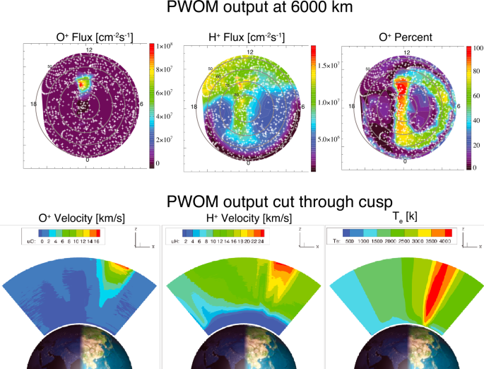
The PWOM result after imposing a cusp region on top of the typical two-cell convection pattern. Top three panels show the global distribution of oxygen ion and proton flux and their ratio at 6000 km. Bottom three panels show the meridian distribution of oxygen ion velocity, proton velocity, and electron temperature through the cusp region (Glocer et al. 2018)
-
2.
Another challenge is to understand the multi-scale dynamics in the ionosphere-magnetosphere system and their roles in various cross-regional/cross-energy couplings. For instance, wave-particle interactions are represented by microscopic physics as the excitation and damping of the waves are usually within milliseconds. But meanwhile, they could influence the macro-scale dynamics like the ring current decay, radiation belt energization, and auroral precipitation that last for hours. Some studies have made important progress in incorporating micro-scale wave dynamics, such as EMIC waves, with macro-scale models (e.g., Jordanova et al. 1997; Khazanov et al. 2003; Gamayunov et al. 2014; Bortnik et al. 2011; Fu et al. 2016). More studies are still needed to self-consistently understand the excitation of various types of magnetospheric plasma waves and their impact on the global dynamics. Recently, Jordanova et al. (2018) developed an end-to-end model of the magnetosphere, the SHIELDS framework, by integrating several physics-based models/techniques across multiple scales. This framework aims to address various fundamental problems across different regimes, ranging from the large-scale global magnetosphere to meso-scale inner magnetosphere and small-scale kinetic zone. Such a framework significantly strengthens the capability of representing the complicated geospace environment and allows for a more complete investigation of the system, including particle injections associated with substorms, plasma accelerations, as well as spacecraft surface charging environment that could impose severe threats to the onboard satellite instrument in the magnetosphere. A system-level consideration of the geospace system by integrating as many processes as possibles in different temporal or spatial scales will be a necessary tool in the future, not only to achieve a comprehensive understanding of the entire system, but also for an operational purpose in space weather application.
-
3.
A third challenge is that field-aligned electric potential drop has long been ignored in global models. As the frozen-in condition is generally satisfied in the magnetosphere, equipotential along magnetic field lines is a common assumption. However, this is not realistic or appropriate for regions where mono-energetic precipitation occurs, such as the auroral zone and dayside cusp. The most significant potential drop appears in regions of upward field-aligned current where electromagnetic energy is converted to plasma energy and dissipation loads in the ionosphere. With the simplified potential distribution in the magnetosphere-ionosphere coupling model, the dissipative effects may be underrepresented in the coupled system. For example, Xi et al. (2016) initiated a step forward by including a electric potential drop into global circulation models and investigated the subsequent effects of the dissipative load. They reported a remarkable difference in the tail reconnection. The nightside X-line moves closer to Earth with the reconnection rate raised by 12%. Furthermore, the ionospheric joule dissipation is reduced by 8%. Their study demonstrated the important role of the potential drop, even only in the auroral zone, in regulating the large-scale dynamics. Future magnetosphere-ionosphere modeling studies should consider this long-neglected field-aligned physics, especially in the auroral and cusp regions. Yet, revealing how the electric potential drop distributes on the global scale and how it varies in time is a near-future task.

Change history
30 December 2022
In Section 3, the dawn auroral polarization streams (DAPS) were mistakenly termed as “dawnside SAPS” twice (in the second paragraph in Page 17 and in the last paragraph in Page 20). It was a mistake. DAPS and dawnside SAPS are two different phenomena: DAPS occur within the auroral zone while the dawnside SAPS occur at subauroral latitudes. The article aimed to describe the DAPS, not the “dawnside SAPS”. The original online version of this article was revised.
11 January 2023
A Correction to this paper has been published: https://doi.org/10.1007/s11214-022-00947-7
References
Aikio AT, Vanhamäki H, Workayehu AB, Virtanen II, Kauristie K, Juusola L, Buchert S, Knudsen D (2018) Swarm satellite and EISCAT radar observations of a plasma flow channel in the auroral oval near magnetic midnight. J Geophys Res Space Phys 123(6):5140–5158. https://doi.org/10.1029/2018JA025409
Anderson PC, Carpenter DL, Tsuruda K, Mukai T, Rich FJ (2001) Multisatellite observations of rapid subauroral ion drifts (said). J Geophys Res Space Phys 106(A12):29585–29599. https://doi.org/10.1029/2001JA000128
Angelopoulos V, Baumjohann W, Kennel CF, Coroniti FV, Kivelson MG, Pellat R, Walker RJ, Lühr H, Paschmann G (1992) Bursty bulk flows in the inner central plasma sheet. J Geophys Res 97(A4):4027. https://doi.org/10.1029/91JA02701
Angelopoulos V, Kennel CF, Coroniti FV, Pellat R, Kivelson MG, Walker RJ, Russell CT, Baumjohann W, Feldman WC, Gosling JT (1994) Statistical characteristics of bursty bulk flow events. J Geophys Res Space Phys 99(A11):21257–21280. https://doi.org/10.1029/94JA01263
Araki T (1994) A Physical Model of the Geomagnetic Sudden Commencement. American Geophysical Union (AGU), pp 183–200. https://doi.org/10.1029/GM081p0183
Archer WE, Knudsen DJ, Burchill JK, Jackel B, Donovan E, Connors M, Juusola L (2017) Birkeland current boundary flows. J Geophys Res Space Phys 122(4):4617–4627. https://doi.org/10.1002/2016JA023789
Bailey SM, Barth CA, Solomon SC (2002) A model of nitric oxide in the lower thermosphere. J Geophys Res Space Phys 107(A8):SIA 22-1–SIA 22-12. https://doi.org/10.1029/2001JA000258
Birn J, Hesse M (2013) The substorm current wedge in MHD simulations. J Geophys Res Space Phys 118(6):3364–3376. https://doi.org/10.1002/jgra.50187
Birn J, Hesse M (2014) The substorm current wedge: further insights from MHD simulations. J Geophys Res Space Phys 119(5):3503–3513. https://doi.org/10.1002/2014JA019863
Birn J, Hesse M, Haerendel G, Baumjohann W, Shiokawa K (1999) Flow braking and the substorm current wedge. J Geophys Res Space Phys 104(A9):19895–19904. https://doi.org/10.1029/1999JA900173
Birn J, Nakamura R, Panov EV, Hesse M (2011) Bursty bulk flows and dipolarization in MHD simulations of magnetotail reconnection. J Geophys Res Space Phys 116(A1):A01210. https://doi.org/10.1029/2010JA016083
Birn J, Liu J, Runov A, Kepko L, Angelopoulos V (2019) On the contribution of dipolarizing flux bundles to the substorm current wedge and to flux and energy transport. J Geophys Res Space Phys 124(7):5408–5420. https://doi.org/10.1029/2019JA026658
Birn J, Borovsky JE, Hesse M, Kepko L (2020) Substorm current wedge: energy conversion and current diversion. J Geophys Res Space Phys 125(8):1–12. https://doi.org/10.1029/2020JA028073
Bortnik J, Omidi N, Chen L, Thorne RM, Horne RB (2011) Saturation characteristics of electromagnetic ion cyclotron waves. J Geophys Res Space Phys 116(A9):A09219. https://doi.org/10.1029/2011JA016638
Cao J, Duan J, Du A, Ma Y, Liu Z, Zhou GC, Yang D, Zhang T, Li X, Massimo V (2008) Characteristics of middle- to low-latitude Pi2 excited by bursty bulk flows. J Geophys Res, Atmos 113(A7):521–532
Cao JB, Yan C, Dunlop M, Reme H, Dandouras I, Zhang T, Yang D, Moiseyev A, Solovyev SI, Wang ZQ (2010) Geomagnetic signatures of current wedge produced by fast flows in a plasma sheet. J Geophys Res, Atmos 115(A8):A08205
Chen L, Jordanova VK, Spasojević M, Thorne RM, Horne RB (2014) Electromagnetic ion cyclotron wave modeling during the geospace environment modeling challenge event. J Geophys Res Space Phys 119(4):2963–2977. https://doi.org/10.1002/2013JA019595
Chen MW, Lemon CL, Guild TB, Keesee AM, Lui A, Goldstein J, Rodriguez JV, Anderson PC (2015a) Effects of modeled ionospheric conductance and electron loss on self-consistent ring current simulations during the 5–7 April 2010 storm. J Geophys Res Space Phys 120(7):5355–5376. https://doi.org/10.1002/2015JA021285
Chen MW, Lemon CL, Orlova K, Shprits Y, Hecht J, Walterscheid RL (2015b) Comparison of simulated and observed trapped and precipitating electron fluxes during a magnetic storm. Geophys Res Lett 42(20):8302–8311. https://doi.org/10.1002/2015GL065737
Chen MW, Lemon CL, Hecht J, Sazykin S, Wolf RA, Boyd A, Valek P (2019) Diffuse auroral electron and ion precipitation effects on RCM-E comparisons with satellite data during the 17 March 2013 storm. J Geophys Res Space Phys 124(6):4194–4216. https://doi.org/10.1029/2019JA026545
Collis P, Häggström I (1991) High-latitude ionospheric response to a geomagnetic sudden commencement. J Atmos Terr Phys 53(3):241–248. https://doi.org/10.1016/0021-9169(91)90108-J
Connor HK, Zesta E, Fedrizzi M, Shi Y, Raeder J, Codrescu MV, Fuller-Rowell TJ (2016) Modeling the ionosphere-thermosphere response to a geomagnetic storm using physics-based magnetospheric energy input: OpenGGCM-CTIM results. J Space Weather Space Clim 6(27):A25. https://doi.org/10.1051/swsc/2016019
Cramer WD, Raeder J, Toffoletto FR, Gilson M, Hu B (2017) Plasma sheet injections into the inner magnetosphere: two-way coupled OpenGGCM-RCM model results. J Geophys Res Space Phys 122(5):5077–5091. https://doi.org/10.1002/2017JA024104
Dungey JW (1961) Interplanetary magnetic field and the auroral zones. Phys Rev Lett 6(2):47–48. https://doi.org/10.1103/PhysRevLett.6.47
Ebihara Y, Fok MC, Immel TJ, Brandt PC (2011) Rapid decay of storm time ring current due to pitch angle scattering in curved field line. J Geophys Res Space Phys 116(A3):A03218. https://doi.org/10.1029/2010JA016000
Engebretson MJ, Murr DL, Hughes WJ, Lühr H, Moretto T, Posch JL, Weatherwax AT, Rosenberg TJ, Maclennan CG, Lanzerotti LJ, Marcucci F, Dennis S, Burns G, Bitterly J, Bitterly M (1999) A multipoint determination of the propagation velocity of a sudden commencement across the polar ionosphere. J Geophys Res Space Phys 104(A10):22433–22451. https://doi.org/10.1029/1999JA900237
Erickson GM, Wolf RA (1980) Is steady convection possible in the Earth’s magnetotail? Geophys Res Lett 7(11):897–900. https://doi.org/10.1029/GL007i011p00897
Eshetu WW, Tu W, Jordanova VK, Cowee M (2021) Quantifying the effect of magnetic field line curvature scattering on the loss of ring current ions. J Geophys Res Space Phys 126(1):1–18. https://doi.org/10.1029/2020JA028497
Fang X, Randall CE, Lummerzheim D, Solomon SC, Mills MJ, Marsh DR, Jackman CH, Wang W, Lu G (2008) Electron impact ionization: a new parameterization for 100 eV to 1 MeV electrons. J Geophys Res Space Phys 113(A9):A09311. https://doi.org/10.1029/2008JA013384
Fok MC, Wolf RA, Spiro RW, Moore TE (2001) Comprehensive computational model of Earth’s ring current. J Geophys Res Space Phys 106:8417–8424. https://doi.org/10.1029/2000JA000235
Fok MC, Buzulukova NY, Chen SH, Glocer A, Nagai T, Valek P, Perez JD (2014) The comprehensive inner magnetosphere-ionosphere model. J Geophys Res Space Phys 119(9):7522–7540. https://doi.org/10.1002/2014JA020239
Foster JC, Burke WJ (2002) SAPS: a new categorization for sub-auroral electric fields. Eos, Trans Am Geophys Union 83(36):393–394. https://doi.org/10.1029/2002EO000289
Foster JC, Vo HB (2002) Average characteristics and activity dependence of the subauroral polarization stream. J Geophys Res Space Phys 107(A12):SIA 16-1–SIA 16-10. https://doi.org/10.1029/2002JA009409
Foster JC, Rideout W, Sandel B, Forrester WT, Rich FJ (2007) On the relationship of SAPS to storm-enhanced density. J Atmos Sol-Terr Phys 69(3):303–313. https://doi.org/10.1016/j.jastp.2006.07.021
Fridman M, Lemaire J (1980) Relationship between auroral electrons fluxes and field aligned electric potential difference. J Geophys Res Space Phys 85:664–670. https://doi.org/10.1029/JA085iA02p00664
Fu X, Cowee MM, Jordanova VK, Gary SP, Reeves GD, Winske D (2016) Predicting electromagnetic ion cyclotron wave amplitude from unstable ring current plasma conditions. J Geophys Res Space Phys 121(11):10,954–10,965. https://doi.org/10.1002/2016JA023303
Fujita S (2019) Response of the Magnetosphere–Ionosphere System to Sudden Changes in Solar Wind Dynamic Pressure, vol 3. Springer, Singapore. https://doi.org/10.1007/s41614-019-0025-1
Fujita S, Tanaka T (2006) Magnetospheric plasma processes during a sudden commencement revealed from a global MHD simulation. In: Magnetospheric ULF Waves: Synthesis and New Directions, vol 169, p 31. https://doi.org/10.1029/169GM05
Fujita S, Tanaka T, Kikuchi T, Fujimoto K, Hosokawa K, Itonaga M (2003a) A numerical simulation of the geomagnetic sudden commencement: 1. Generation of the field-aligned current associated with the preliminary impulse. J Geophys Res Space Phys 108(A12):1416. https://doi.org/10.1029/2002JA009407
Fujita S, Tanaka T, Kikuchi T, Fujimoto K, Itonaga M (2003b) A numerical simulation of the geomagnetic sudden commencement: 2. Plasma processes in the main impulse. J Geophys Res Space Phys 108(A12):1417. https://doi.org/10.1029/2002JA009763
Fujita S, Tanaka T, Kikuchi T, Tsunomura S (2004) A numerical simulation of a negative sudden impulse. Earth Planets Space 56:463–472. https://doi.org/10.1186/BF03352499
Fujita S, Tanaka T, Motoba T (2005) A numerical simulation of the geomagnetic sudden commencement: 3. A sudden commencement in the magnetosphere-ionosphere compound system. J Geophys Res Space Phys 110(A11):A11203. https://doi.org/10.1029/2005JA011055
Fujita S, Yamagishi H, Murata KT, Den M, Tanaka T (2012) A numerical simulation of a negative solar wind impulse: revisited. J Geophys Res Space Phys 117(A9):A09219. https://doi.org/10.1029/2012JA017526
Fuller-Rowell TJ, Rees D (1980) A three-dimensional time-dependent global model of the thermosphere. J Atmos Sci 37:2545–2567. https://doi.org/10.1175/1520-0469(1980)037<2545:ATDTDG>2.0.CO;2
Fuselier SA (2004) Generation of transient dayside subauroral proton precipitation. J Geophys Res 109(A12):A12227. https://doi.org/10.1029/2004JA010393
Galand M, Richmond AD (2001) Ionospheric electrical conductances produced by auroral proton precipitation. J Geophys Res Space Phys 106(A1):117–125. https://doi.org/10.1029/1999JA002001
Gamayunov KV, Engebretson MJ, Zhang M, Rassoul HK (2014) Model of electromagnetic ion cyclotron waves in the inner magnetosphere. J Geophys Res Space Phys 119(9):7541–7565. https://doi.org/10.1002/2014JA020032
Ganushkina NY, Liemohn MW, Dubyagin S (2018) Current systems in the Earth’s magnetosphere. Rev Geophys 56(2):309–332. https://doi.org/10.1002/2017RG000590
Garner TW, Wolf RA, Spiro RW, Thomsen MF, Korth H (2003) Pressure balance inconsistency exhibited in a statistical model of magnetospheric plasma. J Geophys Res Space Phys 108(A8):1331. https://doi.org/10.1029/2003JA009877
Gkioulidou M, Wang CP, Lyons LR, Wolf RA (2009) Formation of the Harang reversal and its dependence on plasma sheet conditions: Rice convection model simulations. J Geophys Res Space Phys 114(A7):A07204. https://doi.org/10.1029/2008JA013955
Gkioulidou M, Wang CP, Wing S, Lyons LR, Wolf RA, Hsu TS (2012) Effect of an MLT dependent electron loss rate on the magnetosphere-ionosphere coupling. J Geophys Res Space Phys 117(A11):A11218. https://doi.org/10.1029/2012JA018032
Glassmeier KH, Heppner C (1992) Traveling magnetospheric convection twin vortices: another case study, global characteristics, and a model. J Geophys Res Space Phys 97(A4):3977–3992. https://doi.org/10.1029/91JA02464
Glocer A (2016) Coupling Ionospheric Outflow into Magnetospheric Models. American Geophysical Union (AGU), pp 195–203. Chap. 15. https://doi.org/10.1002/9781119066880.ch15
Glocer A, Tóth G, Gombosi T, Welling D (2009) Modeling ionospheric outflows and their impact on the magnetosphere, initial results. J Geophys Res Space Phys 114:5216. https://doi.org/10.1029/2009JA014053
Glocer A, Toth G, Fok MC (2018) Including kinetic ion effects in the coupled global ionospheric outflow solution. J Geophys Res Space Phys 123(4):2851–2871. https://doi.org/10.1002/2018JA025241
Grandin M, Battarbee M, Osmane A, Ganse U, Pfau-Kempf Y, Turc L, Brito T, Koskela T, Dubart M, Palmroth M (2019) Hybrid-Vlasov modelling of nightside auroral proton precipitation during southward interplanetary magnetic field conditions. Ann Geophys 37(5):791–806. https://doi.org/10.5194/angeo-37-791-2019
Hao Y, Huang J, Liu W, Zhang D, Xiao Z (2017) Prompt GPS TEC response to magnetospheric compression. J Geophys Res Space Phys 122(4):4357–4366. https://doi.org/10.1002/2017JA023866
Hardy DA, Gussenhoven MS, Holeman E (1985) A statistical model of auroral electron precipitation. J Geophys Res 90(A5):4229. https://doi.org/10.1029/JA090iA05p04229
Hardy DA, Gussenhoven MS, Raistrick R, Mcneil WJ (1987) Statistical and functional representations of the pattern of auroral energy flux, number flux, and conductivity. J Geophys Res, Atmos 92(A11):12275–12294
Hardy DA, Gussenhoven MS, Brautigam D (1989) A statistical model of auroral ion precipitation. J Geophys Res 94(A1):370. https://doi.org/10.1029/JA094iA01p00370
He F, Zhang XX, Wang W, Chen B (2016) Double-peak subauroral ion drifts (DSAIDs). Geophys Res Lett 43(11):5554–5562. https://doi.org/10.1002/2016GL069133
He F, Zhang XX, Wang W, Wan W (2017) Different evolution patterns of subauroral polarization streams (SAPS) during intense storms and quiet time substorms. Geophys Res Lett 44(21):10,796–10,804. https://doi.org/10.1002/2017GL075449
He F, Zhang XX, Wang W, Liu L, Ren ZP, Yue X, Hu L, Wan W, Wang H (2018) Large-scale structure of subauroral polarization streams during the main phase of a severe geomagnetic storm. J Geophys Res Space Phys. https://doi.org/10.1002/2018JA025234
Henderson MG, Reeves GD, Murphree JS (1998) Are north-south aligned auroral structures an ionospheric manifestation of bursty bulk flows? Geophys Res Lett 25(19):3737–3740. https://doi.org/10.1029/98GL02692
Hori T, Shinbori A, Nishitani N, Kikuchi T, Fujita S, Nagatsuma T, Troshichev O, Yumoto K, Moiseyev A, Seki K (2012) Evolution of negative SI-induced ionospheric flows observed by SuperDARN King Salmon HF radar. J Geophys Res Space Phys 117(A12):A12223. https://doi.org/10.1029/2012JA018093
Horvath I, Lovell BC (2017) Investigating the development of double-peak subauroral ion drift (DSAID). J Geophys Res Space Phys 122(4):4526–4542. https://doi.org/10.1002/2016JA023506
Horvath I, Lovell BC (2021) Investigating the coupled magnetosphere-ionosphere-thermosphere (M-I-T) system’s responses to the 20 November 2003 superstorm. J Geophys Res Space Phys 126(9):e2021JA029215. https://doi.org/10.1029/2021JA029215
Hosokawa K, Ogawa Y (2010) Pedersen current carried by electrons in auroral D-region. Geophys Res Lett 37:L18103. https://doi.org/10.1029/2010GL044746
Huang CS, Zhang Y, Wang W, Lin D, Wu Q (2021) Low-latitude zonal ion drifts and their relationship with subauroral polarization streams and auroral return flows during intense magnetic storms. J Geophys Res Space Phys 126(12):e2021JA030001. https://doi.org/10.1029/2021JA030001
Huba JD, Sazykin S, Coster A (2017) SAMI3-RCM simulation of the 17 March 2015 geomagnetic storm. J Geophys Res Space Phys 122(1):1246–1257. https://doi.org/10.1002/2016JA023341
Iijima T, Potemra TA (1978) Large-scale characteristics of field-aligned currents associated with substorms. J Geophys Res Space Phys 83(A2):599–615. https://doi.org/10.1029/JA083iA02p00599
Iijima T, Potemra TA, Zanetti LJ, Bythrow PF (1984) Large-scale Birkeland currents in the dayside polar region during strongly northward IMF: a new Birkeland current system. J Geophys Res Space Phys 89(A9):7441–7452. https://doi.org/10.1029/JA089iA09p07441
Jiang F, Kivelson MG, Strangeway RJ, Khurana KK, Walker R (2015) Ionospheric flow shear associated with the preexisting auroral arc: a statistical study from the fast spacecraft data. J Geophys Res Space Phys 120(6):5194–5213. https://doi.org/10.1002/2013JA019255
Johnstone AD (1978) Pulsating aurora. Nature 274(5667):119–126. https://doi.org/10.1038/274119a0
Jordanova VK, Kozyra JU, Nagy AF, Khazanov GV (1997) Kinetic model of the ring current-atmosphere interactions. J Geophys Res Space Phys 102:14279–14292. https://doi.org/10.1029/96JA03699
Jordanova VK, Farrugia CJ, Thorne RM, Khazanov GV, Reeves GD, Thomsen MF (2001) Modeling ring current proton precipitation by electromagnetic ion cyclotron waves during the May 14–16, 1997, storm. J Geophys Res Space Phys 106:7–22. https://doi.org/10.1029/2000JA002008
Jordanova VK, Miyoshi YS, Zaharia S, Thomsen MF, Reeves GD, Evans DS, Mouikis CG, Fennell JF (2006) Kinetic simulations of ring current evolution during the Geospace Environment Modeling challenge events. J Geophys Res Space Phys 111:A11S10. https://doi.org/10.1029/2006JA011644
Jordanova VK, Spasojevic M, Thomsen MF (2007) Modeling the electromagnetic ion cyclotron wave-induced formation of detached subauroral proton arcs. J Geophys Res Space Phys 112(A8):A08209. https://doi.org/10.1029/2006JA012215
Jordanova VK, Thorne RM, Li W, Miyoshi Y (2010a) Excitation of whistler mode chorus from global ring current simulations. J Geophys Res Space Phys 115(A5):A00F10. https://doi.org/10.1029/2009JA014810
Jordanova VK, Zaharia S, Welling DT (2010b) Comparative study of ring current development using empirical, dipolar, and self-consistent magnetic field simulations. J Geophys Res Space Phys 115(A14):A00J11. https://doi.org/10.1029/2010JA015671
Jordanova VK, Tu W, Chen Y, Morley SK, Panaitescu AD, Reeves GD, Kletzing CA (2016) RAM-SCB simulations of electron transport and plasma wave scattering during the October 2012 “double-dip” storm. J Geophys Res Space Phys 121:8712–8727. https://doi.org/10.1002/2016JA022470
Jordanova V, Delzanno G, Henderson M, Godinez H, Jeffery C, Lawrence E, Morley S, Moulton J, Vernon L, Woodroffe J, Brito T, Engel M, Meierbachtol C, Svyatsky D, Yu Y, Tóth G, Welling D, Chen Y, Haiducek J, Markidis S, Albert J, Birn J, Denton M, Horne R (2018) Specification of the near-Earth space environment with SHIELDS. J Atmos Sol-Terr Phys 177(April 2017):148–159. https://doi.org/10.1016/j.jastp.2017.11.006
Kaeppler SR, Hampton DL, Nicolls MJ, Strømme A, Solomon SC, Hecht JH, Conde MG (2015) An investigation comparing ground-based techniques that quantify auroral electron flux and conductance. J Geophys Res Space Phys 120(10):9038–9056. https://doi.org/10.1002/2015JA021396
Karlsson T, Marklund GT, Blomberg LG, Mäkki A (1998) Subauroral electric fields observed by the Freja satellite: a statistical study. J Geophys Res Space Phys 103(A3):4327–4341. https://doi.org/10.1029/97JA00333
Kasahara S, Miyoshi Y, Yokota S, Mitani T, Kasahara Y, Matsuda S, Kumamoto A, Matsuoka A, Kazama Y, Frey HU, Angelopoulos V, Kurita S, Keika K, Seki K, Shinohara I (2018) Pulsating aurora from electron scattering by chorus waves. Nature 554:337–340. https://doi.org/10.1038/nature25505
Kepko L, McPherron RL, Amm O, Apatenkov S, Baumjohann W, Birn J, Lester M, Nakamura R, Pulkkinen TI, Sergeev V (2015) Substorm current wedge revisited. Space Sci Rev 190(1–4):1–46. https://doi.org/10.1007/s11214-014-0124-9
Kersten T, Horne RB, Glauert SA, Meredith NP, Fraser BJ, Grew RS (2014) Electron losses from the radiation belts caused by EMIC waves. J Geophys Res Space Phys 119(11):8820–8837. https://doi.org/10.1002/2014JA020366
Khazanov GV, Liemohn MW, Newman TS, Fok MC, Spiro RW (2003) Self-consistent magnetosphere-ionosphere coupling: theoretical studies. J Geophys Res Space Phys 108:1122. https://doi.org/10.1029/2002JA009624
Khazanov GV, Glocer A, Sibeck DG, Tripathi AK, Detweiler LG, Avanov LA, Singhal RP (2016) Ionosphere-magnetosphere energy interplay in the regions of diffuse aurora. J Geophys Res Space Phys 121(7):6661–6673. https://doi.org/10.1002/2016JA022403
Khazanov GV, Robinson RM, Zesta E, Sibeck DG, Chu M, Grubbs GA (2018) Impact of precipitating electrons and magnetosphere-ionosphere coupling processes on ionospheric conductance. Space Weather 16(7):829–837. https://doi.org/10.1029/2018SW001837
Kivelson MG, Southwood DJ (1991) Ionospheric traveling vortex generation by solar wind buffeting of the magnetosphere. J Geophys Res Space Phys 96(A2):1661–1667
Knight S (1973) Parallel electric fields. Planet Space Sci 21(5):741–750. https://doi.org/10.1016/0032-0633(73)90093-7
Kunduri BSR, Baker JBH, Ruohoniemi JM, Thomas EG, Shepherd SG, Sterne KT (2017) Statistical characterization of the large-scale structure of the subauroral polarization stream. J Geophys Res Space Phys 122(6):6035–6048. https://doi.org/10.1002/2017JA024131
Liemohn MW (2020) The case for improving the Robinson formulas. J Geophys Res Space Phys 125(10):e2020JA028332. https://doi.org/10.1029/2020JA028332
Lin D, Wang W, Scales WA, Pham K, Liu J, Zhang B, Merkin V, Shi X, Kunduri B, Maimaiti M (2019) SAPS in the 17 March 2013 storm event: initial results from the coupled magnetosphere–ionosphere–thermosphere model. J Geophys Res Space Phys 124(7):6212–6225. https://doi.org/10.1029/2019JA026698
Lin D, Wang W, Merkin VG, Huang C, Oppenheim M, Sorathia K, Pham K, Michael A, Bao S, Wu Q, Zhang Y, Wiltberger M, Toffoletto F, Lyon J, Garretson J (2022) Origin of dawnside subauroral polarization streams during major geomagnetic storms. AGU Adv 3(4):e2022AV000708. https://doi.org/10.1029/2022AV000708
Liu J, Angelopoulos V, Zhou XZ, Runov A, Yao Z (2013) On the role of pressure and flow perturbations around dipolarizing flux bundles. J Geophys Res Space Phys 118(11):7104–7118. https://doi.org/10.1002/2013JA019256
Liu J, Angelopoulos V, Zhou XZ, Yao ZH, Runov A (2015) Cross-tail expansion of dipolarizing flux bundles. J Geophys Res Space Phys 120(4):2516–2530. https://doi.org/10.1002/2015JA020997
Liu J, Angelopoulos V, Yao Z, Chu X, Zhou XZ, Runov A (2018a) The Current System of Dipolarizing Flux Bundles and Their Role as Wedgelets in the Substorm Current Wedge. American Geophysical Union (AGU), pp 323–337. Chap. 19. https://doi.org/10.1002/9781119324522.ch19
Liu J, Lyons LR, Archer WE, Gallardo-Lacourt B, Nishimura Y, Zou Y, Gabrielse C, Weygand JM (2018b) Flow shears at the poleward boundary of omega bands observed during conjunctions of swarm and THEMIS ASI. Geophys Res Lett 45(3):1218–1227. https://doi.org/10.1002/2017GL076485
Liu J, Lyons LR, Wang CP, Hairston MR, Zhang Y, Zou Y (2020) Dawnside auroral polarization streams. J Geophys Res Space Phys 125(8):e2019JA027742. https://doi.org/10.1029/2019JA027742
Lotko W, Smith RH, Zhang B, Ouellette JE, Brambles OJ, Lyon JG (2014) Ionospheric control of magnetotail reconnection. Science 345(6193):184–187. https://doi.org/10.1126/science.1252907
Lühr H, Lockwood M, Sandholt PE, Hansen TL, Moretto T (1996) Multi-instrument ground-based observations of a travelling convection vortices event. Ann Geophys 14(2):162–181
Lui ATY (1996) Current disruption in the Earth’s magnetosphere: observations and models. J Geophys Res Space Phys 101(A6):13067–13088. https://doi.org/10.1029/96JA00079
Lyon JG, Fedder JA, Mobarry CM (2004) The Lyon-Fedder-Mobarry (LFM) global MHD magnetospheric simulation code. J Atmos Sol-Terr Phys 66(15–16):1333–1350. https://doi.org/10.1016/j.jastp.2004.03.020
Lyons LR, Evans DS, Lundin R (1979) An observed relation between magnetic field aligned electric fields and downward electron energy fluxes in the vicinity of auroral forms. J Geophys Res Space Phys 84(A2):457–461. https://doi.org/10.1029/JA084iA02p00457
Lysak RL, Dh L (1992) Response of the dipole magnetosphere to pressure pulses. Geophys Res Lett 19(9):937–940. https://doi.org/10.1029/92GL00625
Lysak RL, Song Y, Lee DH (1994) Generation of ULF waves by fluctuations in the magnetopause position. In: Engebretson MJ, Takahashi K, Scholer M (eds) Solar Wind Sources of Magnetospheric Ultra-Low-Frequency Waves, p 273
McGranaghan R, Knipp DJ, Matsuo T, Cousins E (2016) Optimal interpolation analysis of high-latitude ionospheric Hall and Pedersen conductivities: application to assimilative ionospheric electrodynamics reconstruction. J Geophys Res Space Phys 121(5):4898–4923. https://doi.org/10.1002/2016JA022486
McPherron RL, Russell CT, Aubry MP (1973) Satellite studies of magnetospheric substorms on August 15, 1968: 9. Phenomenological model for substorms. J Geophys Res 78(16):3131–3149. https://doi.org/10.1029/JA078i016p03131
Meredith NP, Horne RB, Thorne RM, Anderson RR (2009) Survey of upper band chorus and ECH waves: implications for the diffuse aurora. J Geophys Res Space Phys 114(A7):A07218. https://doi.org/10.1029/2009JA014230
Merkin VG, Lyon JG (2010) Effects of the low-latitude ionospheric boundary condition on the global magnetosphere. J Geophys Res Space Phys 115(A10):A10202. https://doi.org/10.1029/2010JA015461
Merkin VG, Sharma AS, Papadopoulos K, Milikh G, Lyon J, Goodrich C (2005) Global MHD simulations of the strongly driven magnetosphere: modeling of the transpolar potential saturation. J Geophys Res Space Phys 110(A9):1–11. https://doi.org/10.1029/2004JA010993
Merkin VG, Panov EV, Sorathia KA, Ukhorskiy AY (2019) Contribution of bursty bulk flows to the global dipolarization of the magnetotail during an isolated substorm. J Geophys Res Space Phys 124(11):8647–8668. https://doi.org/10.1029/2019JA026872
Mishin EV (2013) Interaction of substorm injections with the subauroral geospace: 1. Multispacecraft observations of SAID. J Geophys Res Space Phys 118(9):5782–5796. https://doi.org/10.1002/jgra.50548
Mishin E, Nishimura Y, Foster J (2017) SAPS/SAID revisited: a causal relation to the substorm current wedge. J Geophys Res Space Phys 122(8):8516–8535. https://doi.org/10.1002/2017JA024263
Miyoshi Y, Sakaguchi K, Shiokawa K, Evans D, Albert J, Connors M, Jordanova V (2008) Precipitation of radiation belt electrons by EMIC waves, observed from ground and space. Geophys Res Lett 35(23):L23101. https://doi.org/10.1029/2008GL035727
Miyoshi Y, Saito S, Seki K, Nishiyama T, Kataoka R, Asamura K, Katoh Y, Ebihara Y, Sakanoi T, Hirahara M, Oyama S, Kurita S, Santolik O (2015a) Relation between fine structure of energy spectra for pulsating aurora electrons and frequency spectra of whistler mode chorus waves. J Geophys Res Space Phys 120:7728–7736. https://doi.org/10.1002/2015JA021562
Miyoshi Y, Oyama S, Saito S, Kurita S, Fujiwara H, Kataoka R, Ebihara Y, Kletzing C, Reeves G, Santolik O, Clilverd M, Rodger CJ, Turunen E, Tsuchiya F (2015b) Energetic electron precipitation associated with pulsating aurora: EISCAT and Van Allen Probe observations. J Geophys Res Space Phys 120(4):2754–2766. https://doi.org/10.1002/2014JA020690
Moretto T, Ridley AJ, Engebretson MJ, Rasmussen O (2000) High-latitude ionospheric response to a sudden impulse event during northward IMF conditions. J Geophys Res Space Phys 105(A2):2521–2532. https://doi.org/10.1029/1999JA900475
Mukhopadhyay A, Welling DT, Liemohn MW, Ridley AJ, Chakraborty S, Anderson BJ (2020) Conductance model for extreme events: impact of auroral conductance on space weather forecasts. Space Weather 18(11):1–27. https://doi.org/10.1029/2020SW002551
Nakamura R, Baumjohann W, Schró¶del R, Brittnacher M, Sergeev VA, Kubyshkina M, Mukai T, Liou K (2001) Earthward flow bursts, auroral streamers, and small expansions. J Geophys Res Space Phys 106(A6):10791–10802. https://doi.org/10.1029/2000JA000306
Nakamura R, Amm O, Laakso H, Draper NC, Lester M, Grocott A, Klecker B, McCrea IW, Balogh A, Rème H, André M (2005) Localized fast flow disturbance observed in the plasma sheet and in the ionosphere. Ann Geophys 23(2):553–566. https://doi.org/10.5194/angeo-23-553-2005
Newell PT, Feldstein YI, Galperin YI, Meng CI (1996) Morphology of nightside precipitation. J Geophys Res Space Phys 101(A5):10737–10748. https://doi.org/10.1029/95JA03516
Newell PT, Sotirelis T, Wing S (2009) Diffuse, monoenergetic, and broadband aurora: the global precipitation budget. J Geophys Res Space Phys 114(A9):A09207. https://doi.org/10.1029/2009JA014326
Newell PT, Liou K, Zhang Y, Sotirelis T, Paxton LJ, Mitchell EJ (2014) OVATION Prime-2013: extension of auroral precipitation model to higher disturbance levels. Space Weather 12(6):368–379. https://doi.org/10.1002/2014SW001056
Ni B, Thorne RM, Zhang X, Bortnik J, Pu Z, Xie L, Hu Zj, Han D, Shi R, Zhou C, Gu X (2016) Origins of the Earth’s diffuse auroral precipitation. Space Sci Rev 200(1):205–259. https://doi.org/10.1007/s11214-016-0234-7
Nishimura Y, Bortnik J, Li W, Lyons LR, Donovan EF, Angelopoulos V, Mende SB (2014) Evolution of nightside subauroral proton aurora caused by transient plasma sheet flows. J Geophys Res Space Phys 119(7):5295–5304. https://doi.org/10.1002/2014JA020029
Nishimura Y, Lyons LR, Gabrielse C, Weygand JM, Donovan EF, Angelopoulos V (2020) Relative contributions of large-scale and wedgelet currents in the substorm current wedge. Earth Planets Space 72(1):106. https://doi.org/10.1186/s40623-020-01234-x
Ogino T (1986) A three-dimensional MHD simulation of the interaction of the solar wind with the Earth’s magnetosphere: the generation of field-aligned currents. J Geophys Res Space Phys 91(A6):6791–6806. https://doi.org/10.1029/JA091iA06p06791
Ozturk DS, Zou S, Ridley AJ, Slavin JA (2018) Modeling study of the geospace system response to the solar wind dynamic pressure enhancement on 17 March 2015. J Geophys Res Space Phys 123(4):2974–2989. https://doi.org/10.1002/2017JA025099
Palin L, Jacquey C, Opgenoorth H, Connors M, Sergeev V, Sauvaud JA, Nakamura R, Reeves GD, Singer HJ, Angelopoulos V, Turc L (2015) Three-dimensional current systems and ionospheric effects associated with small dipolarization fronts. J Geophys Res Space Phys 120(5):3739–3757. https://doi.org/10.1002/2015JA021040
Palin L, Opgenoorth HJ, Ågren K, Zivkovic T, Sergeev VA, Kubyshkina MV, Nikolaev A, Kauristie K, Kamp M, Amm O, Milan SE, Imber SM, Facskó G, Palmroth M, Nakamura R (2016) Modulation of the substorm current wedge by bursty bulk flows: 8 September 2002—revisited. J Geophys Res Space Phys 121(5):4466–4482. https://doi.org/10.1002/2015JA022262
Perlongo NJ, Ridley AJ, Liemohn MW, Katus RM (2017) The effect of ring current electron scattering rates on magnetosphere-ionosphere coupling. J Geophys Res Space Phys 122:4168–4189. https://doi.org/10.1002/2016JA023679
Picone JM, Hedin AE, Drob DP, Aikin AC (2002) NRLMSISE-00 empirical model of the atmosphere: statistical comparisons and scientific issues. J Geophys Res Space Phys 107(A12):SIA 15-1–SIA 15-16. https://doi.org/10.1029/2002JA009430
Powell KG, Roe PL, Linde TJ, Gombosi TI, Zeeuw DLD (1999) A solution-adaptive upwind scheme for ideal magnetohydrodynamics. J Comput Phys 154:284
Pytte T, Mcpherron RL, Kokubun S (1976) The ground signatures of the expansion phase during multiple onset substorms. Planet Space Sci 24(12):1115–1132
Raeder J, McPherron RL, Frank LA, Kokubun S, Lu G, Mukai T, Paterson WR, Sigwarth JB, Singer HJ, Slavin JA (2001) Global simulation of the Geospace Environment Modeling substorm challenge event. J Geophys Res Space Phys 106:381–396. https://doi.org/10.1029/2000JA000605
Raeder J, Larson D, Li W, Kepko EL, Fuller-Rowell T (2008) OpenGGCM simulations for the THEMIS mission. Space Sci Rev 141(1–4):535–555. https://doi.org/10.1007/s11214-008-9421-5
Raeder J, Cramer WD, Jensen J, Fuller-Rowell T, Maruyama N, Toffoletto F, Vo H (2016) Sub-auroral polarization streams: a complex interaction between the magnetosphere, ionosphere, and thermosphere. J Phys Conf Ser 767(1):012021
Ream JB, Walker RJ, Ashour-Abdalla M, El-Alaoui M, Wiltberger M, Kivelson MG, Goldstein ML (2015) Propagation of Pi2 pulsations through the braking region in global MHD simulations. J Geophys Res Space Phys 120(12):10574–10591. https://doi.org/10.1002/2015JA021572
Rees D, Fuller-Rowell TJ (1988) Understanding the transport of atomic oxygen within the thermosphere, using a numerical global thermospheric model. Planet Space Sci 36:935–948. https://doi.org/10.1016/0032-0633(88)90101-8
Richmond AD, Ridley EC, Roble RG (1992) A thermosphere/ionosphere general circulation model with coupled electrodynamics. Geophys Res Lett 19(6):601–604. https://doi.org/10.1029/92GL00401
Ridley A, Gombosi T, Dezeeuw D (2004) Ionospheric control of the magnetosphere: conductance. Ann Geophys 22:567–584. https://doi.org/10.5194/angeo-22-567-2004
Ridley AJ, Deng Y, Tóth G (2006) The global ionosphere thermosphere model. J Atmos Sol-Terr Phys 68(8):839–864. https://doi.org/10.1016/j.jastp.2006.01.008
Ritter P, Lühr H (2008) Near-Earth magnetic signature of magnetospheric substorms and an improved substorm current model. Ann Geophys 26(9):2781–2793
Robinson RM, Vondrak RR, Miller K, Dabbs T, Hardy D (1987) On calculating ionospheric conductances from the flux and energy of precipitating electrons. J Geophys Res Space Phys 92:2565–2569. https://doi.org/10.1029/JA092iA03p02565
Robinson RM, Kaeppler SR, Zanetti L, Anderson B, Vines SK, Korth H, Fitzmaurice A (2020) Statistical relations between auroral electrical conductances and field-aligned currents at high latitudes. J Geophys Res Space Phys 125(7):1–16. https://doi.org/10.1029/2020JA028008
Roble RG, Ridley EC, Richmond AD, Dickinson RE (1988) A coupled thermosphere/ionosphere general circulation model. Geophys Res Lett 15(12):1325–1328. https://doi.org/10.1029/GL015i012p01325
Saikin AA, Zhang JC, Allen RC, Smith CW, Kistler LM, Spence HE, Torbert RB, Kletzing CA, Jordanova VK (2015) The occurrence and wave properties of \(\text{H}^{+}\)-, \(\text{He}^{+}\)-, and \(\text{O}^{+}\)-band EMIC waves observed by the Van Allen Probes. J Geophys Res Space Phys 120(9):7477–7492. https://doi.org/10.1002/2015JA021358
Samsonov AA, Sibeck DG, Yu Y (2010) Transient changes in magnetospheric-ionospheric currents caused by the passage of an interplanetary shock: northward interplanetary magnetic field case. J Geophys Res Space Phys 115(A5):A05207. https://doi.org/10.1029/2009JA014751
Sergeev V, Sazhina E, Tsyganenko N, Lundblad J, Søraas F (1983) Pitch-angle scattering of energetic protons in the magnetotail current sheet as the dominant source of their isotropic precipitation into the nightside ionosphere. Planet Space Sci 31(10):1147–1155. https://doi.org/10.1016/0032-0633(83)90103-4
Sergeev VA, Malkov M, Mursula K (1993) Testing the isotropic boundary algorithm method to evaluate the magnetic field configuration in the tail. J Geophys Res Space Phys 98(A5):7609–7620. https://doi.org/10.1029/92JA02587
Sergeev VA, Angelopoulos V, Gosling JT, Cattell CA, Russell CT (1996) Detection of localized, plasma-depleted flux tubes or bubbles in the midtail plasma sheet. J Geophys Res Space Phys 101(A5):10817–10826. https://doi.org/10.1029/96JA00460
Sergeev VA, Liou K, Meng CI, Newell PT, Brittnacher M, Parks G, Reeves GD (1999) Development of auroral streamers in association with localized impulsive injections to the inner magnetotail. Geophys Res Lett 26(3):417–420. https://doi.org/10.1029/1998GL900311
Sergeev VA, Tsyganenko NA, Smirnov MV, Nikolaev AV, Singer HJ, Baumjohann W (2011) Magnetic effects of the substorm current wedge in a “spread-out wire” model and their comparison with ground, geosynchronous, and tail lobe data. J Geophys Res Space Phys 116(A7):A07218. https://doi.org/10.1029/2011JA016471
Sergeev VA, Nikolaev AV, Tsyganenko NA, Angelopoulos V, Runov AV, Singer HJ, Yang J (2014) Testing a two-loop pattern of the substorm current wedge (SCW2L). J Geophys Res Space Phys 119(2):947–963. https://doi.org/10.1002/2013JA019629
Shiokawa K, Baumjohann W, Haerendel G, Paschmann G, Fennell JF, Friis-Christensen E, Lühr H, Reeves GD, Russell CT, Sutcliffe PR, Takahashi K (1998) High-speed ion flow, substorm current wedge, and multiple Pi 2 pulsations. J Geophys Res Space Phys 103(A3):4491–4507. https://doi.org/10.1029/97JA01680
Shreedevi PR, Yu Y, Ni B, Saikin A, Jordanova VK (2021) Simulating the ion precipitation from the inner magnetosphere by H-band and He-band electro magnetic ion cyclotron (EMIC) waves. J Geophys Res Space Phys 126:e2020JA028553. https://doi.org/10.1029/2020ja028553
Sibeck DG, Trivedi NB, Zesta E, Decker RB, Singer HJ, Szabo A, Tachihara H, Watermann J (2003) Pressure-pulse interaction with the magnetosphere and ionosphere. J Geophys Res Space Phys 108(A2):1095. https://doi.org/10.1029/2002JA009675
Solomon SC (2001) Auroral particle transport using Monte Carlo and hybrid methods. J Geophys Res Space Phys 106(A1):107–116. https://doi.org/10.1029/2000JA002011
Solomon SC (2017) Global modeling of thermospheric airglow in the far ultraviolet. J Geophys Res Space Phys 122(7):7834–7848. https://doi.org/10.1002/2017JA024314
Solomon SC, Hays PB, Abreu VJ (1988) The auroral 6300 Å emission: observations and modeling. J Geophys Res Space Phys 93(A9):9867–9882. https://doi.org/10.1029/JA093iA09p09867
Southwood DJ, Wolf RA (1978) An assessment of the role of precipitation in magnetospheric convection. J Geophys Res Space Phys 83(A11):5227–5232. https://doi.org/10.1029/JA083iA11p05227
Spiro RW, Heelis RA, Hanson WB (1978) Ion convection and the formation of the mid-latitude \(F\) region ionization trough. J Geophys Res Space Phys 83(A9):4255–4264. https://doi.org/10.1029/JA083iA09p04255
Spiro RW, Heelis RA, Hanson WB (1979) Rapid subauroral ion drifts observed by Atmosphere Explorer C. Geophys Res Lett 6(8):657–660. https://doi.org/10.1029/GL006i008p00657
Strickland DJ, Daniell RE Jr, Jasperse JR, Basu B (1993) Transport-theoretic model for the electron-proton-hydrogen atom aurora: 2. Model results. J Geophys Res Space Phys 98(A12):21533–21548. https://doi.org/10.1029/93JA01645
Sun WJ, Fu SY, Parks GK, Liu J, Yao ZH, Shi QQ, Zong QG, Huang SY, Pu ZY, Xiao T (2013) Field-aligned currents associated with dipolarization fronts. Geophys Res Lett 40(17):4503–4508. https://doi.org/10.1002/grl.50902
Takeuchi T, Araki T, Luehr H, Rasmussen O, Watermann J, Milling DK, Mann IR, Yumoto K, Shiokawa K, Nagai T (2000) Geomagnetic negative sudden impulse due to a magnetic cloud observed on May 13, 1995. J Geophys Res Space Phys 105(A8):18835–18846. https://doi.org/10.1029/2000JA900055
Takeuchi T, Araki T, Viljanen A, Watermann J (2002) Geomagnetic negative sudden impulses: interplanetary causes and polarization distribution. J Geophys Res Space Phys 107(A7):SMP 7-1–SMP 7-14. https://doi.org/10.1029/2001JA900152
Tamao T (1964) The structure of three-dimensional hydromagnetic waves in a uniform cold plasma. J Geomagn Geoelectr 16(2):89–114. https://doi.org/10.5636/jgg.16.89
Tanaka T (2000) The state transition model of the substorm onset. J Geophys Res Space Phys 105:21081. https://doi.org/10.1029/2000JA900061
Tian X, Yu Y, Yue C (2020) Statistical survey of storm-time energetic particle precipitation. J Atmos Sol-Terr Phys 199:105204. https://doi.org/10.1016/j.jastp.2020.105204
Tian X, Yu Y, Zhu M, Ma L, Cao J, PR S, Jordanova VK, Solomon SC (2022) Effects of EMIC wave-driven proton precipitation on the ionosphere. J Geophys Res Space Phys 127(2):1–15. https://doi.org/10.1029/2021JA030101
Toffoletto F, Sazykin S, Spiro R, Wolf R (2003) Inner magnetospheric modeling with the Rice Convection Model. Space Sci Rev 107:175–196. https://doi.org/10.1023/A:1025532008047
Tóth G, van der Holst B, Sokolov IV, de Zeeuw DL, Gombosi TI, Fang F, Manchester WB, Meng X, Najib D, Powell KG, Stout QF, Glocer A, Ma YJ, Opher M (2012) Adaptive numerical algorithms in space weather modeling. J Comput Phys 231:870–903. https://doi.org/10.1016/j.jcp.2011.02.006
Tu W, Cowee MM, Liu K (2014) Modeling the loss of inner belt protons by magnetic field line curvature scattering. J Geophys Res Space Phys 119(7):5638–5650. https://doi.org/10.1002/2014JA019864
Turunen E, Kero A, Verronen PT, Miyoshi Y, Oyama SI, Saito S (2016) Mesospheric ozone destruction by high-energy electron precipitation associated with pulsating aurora. J Geophys Res, Atmos 121(19):11,852–11,861. https://doi.org/10.1002/2016JD025015
Varney RH, Wiltberger M, Zhang B, Lotko W, Lyon J (2016) Influence of ion outflow in coupled geospace simulations: 1. Physics-based ion outflow model development and sensitivity study. J Geophys Res Space Phys 121(10):9671–9687. https://doi.org/10.1002/2016JA022777
Vasyliunas VM (1970) Mathematical models of magnetospheric convection and its coupling to the ionosphere. In: McCormack BM, Renzini A (eds) Particles and Field in the Magnetosphere. Astrophysics and Space Science Library, vol 17, p 60. https://doi.org/10.1007/978-94-010-3284-1_6
Vondrak R, Robinson R (1985) Inference of high-latitude ionization and conductivity from AE-C measurements of auroral electron fluxes. J Geophys Res Space Phys 90(A8):7505–7512. https://doi.org/10.1029/JA090iA08p07505
Wang Z, Zou S (2022) COMPASS: a new conductance model based on PFISR and SWARM satellite observations. Space Weather 20(2):e2021SW002958. https://doi.org/10.1029/2021SW002958
Wei D, Yu Y, He F (2019a) The magnetospheric driving source of double-peak subauroral ion drifts: double ring current pressure peaks. Geophys Res Lett 46(13):7079–7087. https://doi.org/10.1029/2019GL083186
Wei D, Yu Y, Ridley AJ, Cao J, Dunlop MW (2019b) Multi-point observations and modeling of subauroral polarization streams (SAPS) and double-peak subauroral ion drifts (DSAIDs): a case study. Adv Space Res 63(11):3522–3535. https://doi.org/10.1016/j.asr.2019.02.004
Wei D, Dunlop MW, Yang J, Dong X, Yu Y, Wang T (2021) Intense dB/dt variations driven by near-Earth bursty bulk flows (BBFs): a case study. Geophys Res Lett 48(4):e2020GL091781. https://doi.org/10.1029/2020GL091781
Welling DT, Barakat AR, Eccles JV, Schunk RW, Chappell CR (2016) Coupling the Generalized Polar Wind Model to Global Magnetohydrodynamics. American Geophysical Union (AGU), pp 179–194. Chap. 14. https://doi.org/10.1002/9781119066880.ch14
Xi S, Lotko W, Zhang B, Wiltberger M, Lyon J (2016) Effects of auroral potential drops on plasma sheet dynamics. J Geophys Res Space Phys 121(11):11,129–11,144. https://doi.org/10.1002/2016JA022856
Yahnin AG, Popova TA, Demekhov AG, Lubchich AA, Matsuoka A, Asamura K, Miyoshi Y, Yokota S, Kasahara S, Keika K, Hori T, Tsuchiya F, Kumamoto A, Kasahara Y, Shoji M, Kasaba Y, Nakamura S, Shinohara I, Kim H, Noh S, Raita T (2021) Evening side EMIC waves and related proton precipitation induced by a substorm. J Geophys Res Space Phys 126(7):e2020JA029091. https://doi.org/10.1029/2020JA029091
Yahnina TA, Yahnin AG (2014) Proton precipitation to the equator of the isotropic boundary during the geomagnetic storm on November 20–29, 2003. Cosm Res 52(1):79–85. https://doi.org/10.1134/S0010952514010092
Yang J, Toffoletto FR, Wolf RA, Sazykin S, Ontiveros PA, Weygand JM (2012) Large-scale current systems and ground magnetic disturbance during deep substorm injections. J Geophys Res Space Phys 117(A4):A04223. https://doi.org/10.1029/2011JA017415
Yang J, Toffoletto FR, Wolf RA (2014) RCM-E simulation of a thin arc preceded by a north-south-aligned auroral streamer. Geophys Res Lett 41(8):2695–2701. https://doi.org/10.1002/2014GL059840
Yao ZH, Pu ZY, Fu SY, Angelopoulos V, Kubyshkina M, Xing X, Lyons L, Nishimura Y, Xie L, Wang XG, Xiao CJ, Cao X, Liu J, Zhang H, Nowada M, Zong QG, Guo RL, Zhong J, Li JX (2012) Mechanism of substorm current wedge formation: THEMIS observations. Geophys Res Lett 39(13):L13102. https://doi.org/10.1029/2012GL052055
Yao Z, Sun WJ, Fu SY, Pu ZY, Liu J, Angelopoulos V, Zhang XJ, Chu XN, Shi QQ, Guo RL, Zong QG (2013a) Current structures associated with dipolarization fronts. J Geophys Res Space Phys 118(11):6980–6985. https://doi.org/10.1002/2013JA019290
Yao ZH, Angelopoulos V, Pu ZY, Fu SY, Kubyshkina M, Liu J, Chu XN, Nishimura T, Cao X, Du AM, Yue C, Shi QQ, Wei Y (2013b) Conjugate observations of flow diversion in the magnetotail and auroral arc extension in the ionosphere. J Geophys Res Space Phys 118(8):4811–4816. https://doi.org/10.1002/jgra.50419
Yu Y, Ridley AJ (2009) The response of the magnetosphere-ionosphere system to a sudden dynamic pressure enhancement under southward IMF conditions. Ann Geophys 27(12):4391–4407. https://doi.org/10.5194/angeo-27-4391-2009
Yu YQ, Ridley AJ (2011) Understanding the response of the ionosphere-magnetosphere system to sudden solar wind density increases. J Geophys Res Space Phys 116(A4):A04210. https://doi.org/10.1029/2010JA015871
Yu Y, Jordanova V, Zaharia S, Koller J, Zhang J, Kistler LM (2012) Validation study of the magnetically self-consistent inner magnetosphere model RAM-SCB. J Geophys Res Space Phys 117:A03222. https://doi.org/10.1029/2011JA017321
Yu Y, Jordanova V, Zou S, Heelis R, Ruohoniemi M, Wygant J (2015) Modeling subauroral polarization streams during the 17 March 2013 storm. J Geophys Res Space Phys 120(3):1738–1750. https://doi.org/10.1002/2014JA020371
Yu Y, Jordanova VK, Ridley AJ, Albert JM, Horne RB, Jeffery CA (2016) A new ionospheric electron precipitation module coupled with RAM-SCB within the geospace general circulation model. J Geophys Res Space Phys 121(9):8554–8575. https://doi.org/10.1002/2016JA022585
Yu Y, Cao J, Fu H, Lu H, Yao Z (2017a) The effects of bursty bulk flows on global-scale current systems. J Geophys Res Space Phys 122(6):6139–6149. https://doi.org/10.1002/2017JA024168
Yu Y, Jordanova VK, Ridley AJ, Toth G, Heelis R (2017b) Effects of electric field methods on modeling the midlatitude ionospheric electrodynamics and inner magnetosphere dynamics. J Geophys Res Space Phys 122(5):5321–5338. https://doi.org/10.1002/2016JA023850
Yu Y, Jordanova VK, McGranaghan RM, Solomon SC (2018) Self-consistent modeling of electron precipitation and responses in the ionosphere: application to low-altitude energization during substorms. Geophys Res Lett 45(13):6371–6381. https://doi.org/10.1029/2018GL078828
Yu Y, Tian X, Jordanova VK (2020) The effects of field line curvature (FLC) scattering on ring current dynamics and isotropic boundary. J Geophys Res Space Phys 125(8):e2020JA027830. https://doi.org/10.1029/2020ja027830
Yuan Z, Deng X, Lin X, Pang Y, Zhou M, Décréau PME, Trotignon JG, Lucek E, Frey HU, Wang J (2010) Link between EMIC waves in a plasmaspheric plume and a detached sub-auroral proton arc with observations of Cluster and IMAGE satellites. Geophys Res Lett 37(7):L07108. https://doi.org/10.1029/2010GL042711
Yuan Z, Xiong Y, Li H, Huang S, Qiao Z, Wang Z, Zhou M, Wang D, Deng X, Raita T, Wang J (2014) Influence of precipitating energetic ions caused by EMIC waves on the subauroral ionospheric E region during a geomagnetic storm. J Geophys Res Space Phys 119(10):8462–8471. https://doi.org/10.1002/2014JA020303
Yue C, Wang CP, Lyons L, Liang J, Donovan EF, Zaharia SG, Henderson M (2014) Current sheet scattering and ion isotropic boundary under 3-D empirical force-balanced magnetic field. J Geophys Res Space Phys 119(10):8202–8211. https://doi.org/10.1002/2014JA020172
Zaharia S, Jordanova VK, Welling D, Tóth G (2010) Self-consistent inner magnetosphere simulation driven by a global MHD model. J Geophys Res Space Phys 115:A12228. https://doi.org/10.1029/2010JA015915
Zesta E, Lyons LR, Donovan E (2000) The auroral signature of earthward flow bursts observed in the magnetotail. Geophys Res Lett 27(20):3241–3244. https://doi.org/10.1029/2000GL000027
Zhang B, Brambles OJ (2021) Polar Cap \(\text{O}^{+}\) Ion Outflow and Its Impact on Magnetospheric Dynamics. American Geophysical Union (AGU), pp 83–114. Chap. 5. https://doi.org/10.1002/9781119815617.ch5
Zhang B, Lotko W, Brambles O, Wiltberger M, Lyon J (2015a) Electron precipitation models in global magnetosphere simulations. J Geophys Res Space Phys 120:1035–1056. https://doi.org/10.1002/2014JA020615
Zhang SR, Erickson PJ, Foster JC, Holt JM, Coster AJ, Makela JJ, Noto J, Meriwether JW, Harding BJ, Riccobono J, Kerr RB (2015b) Thermospheric poleward wind surge at midlatitudes during great storm intervals. Geophys Res Lett 42(13):5132–5140. https://doi.org/10.1002/2015GL064836
Zhang XJ, Li W, Thorne RM, Angelopoulos V, Bortnik J, Kletzing CA, Kurth WS, Hospodarsky GB (2016) Statistical distribution of EMIC wave spectra: observations from Van Allen Probes. Geophys Res Lett 43(24):12,348–12,355. https://doi.org/10.1002/2016GL071158
Zheng Y, Brandt PC, Lui ATY, Fok MC (2008) On ionospheric trough conductance and subauroral polarization streams: simulation results. J Geophys Res Space Phys 113(A4):A04209. https://doi.org/10.1029/2007JA012532
Zhu M, Yu Y, Tian X, Shreedevi PR, Jordanova VK (2021) On the ion precipitation due to field line curvature (FLC) and EMIC wave scattering and their subsequent impact on ionospheric electrodynamics. J Geophys Res Space Phys 126(3):1–17. https://doi.org/10.1029/2020JA028812
Zou S, Lyons LR, Wang CP, Boudouridis A, Ruohoniemi JM, Anderson PC, Dyson PL, Devlin JC (2009) On the coupling between the Harang reversal evolution and substorm dynamics: a synthesis of SuperDARN, DMSP, and IMAGE observations. J Geophys Res Space Phys 114(A1):A01205. https://doi.org/10.1029/2008JA013449
Zou S, Moldwin MB, Ridley AJ, Nicolls MJ, Coster AJ, Thomas EG, Ruohoniemi JM (2014) On the generation/decay of the storm-enhanced density plumes: role of the convection flow and field-aligned ion flow. J Geophys Res Space Phys 119(10):8543–8559. https://doi.org/10.1002/2014JA020408
Zou S, Ozturk D, Varney R, Reimer A (2017) Effects of sudden commencement on the ionosphere: PFISR observations and global MHD simulation. Geophys Res Lett 44(7):3047–3058. https://doi.org/10.1002/2017GL072678
Acknowledgements
The work at Beihang University is supported by the National Nature Science Foundation of China (NSFC) Grants 41821003 and 41974192, and by the Fundamental Research Funds for the Central Universities. The work at Los Alamos was conducted under the auspices of the US Department of Energy with partial support from NSF grant IAA2027951.
Author information
Authors and Affiliations
Ethics declarations
Competing Interests
The authors declare no competing interests.
Additional information
Publisher’s Note
Springer Nature remains neutral with regard to jurisdictional claims in published maps and institutional affiliations.
In Section 3, the dawn auroral polarization streams (DAPS) were mistakenly termed as “dawnside SAPS” twice (in the second paragraph in Page 17 and in the last paragraph in Page 20). It was a mistake. DAPS and dawnside SAPS are two different phenomena: DAPS occur within the auroral zone while the dawnside SAPS occur at subauroral latitudes. The article aimed to describe the DAPS, not the “dawnside SAPS”. The original online version of this article was revised.
Rights and permissions
Open Access This article is licensed under a Creative Commons Attribution 4.0 International License, which permits use, sharing, adaptation, distribution and reproduction in any medium or format, as long as you give appropriate credit to the original author(s) and the source, provide a link to the Creative Commons licence, and indicate if changes were made. The images or other third party material in this article are included in the article’s Creative Commons licence, unless indicated otherwise in a credit line to the material. If material is not included in the article’s Creative Commons licence and your intended use is not permitted by statutory regulation or exceeds the permitted use, you will need to obtain permission directly from the copyright holder. To view a copy of this licence, visit http://creativecommons.org/licenses/by/4.0/.
About this article

Cite this article
Yu, Y., Cao, J., Pu, Z. et al. Meso-Scale Electrodynamic Coupling of the Earth Magnetosphere-Ionosphere System. Space Sci Rev 218, 74 (2022). https://doi.org/10.1007/s11214-022-00940-0
Received:
Accepted:
Published:
DOI: https://doi.org/10.1007/s11214-022-00940-0