A complex structure-preserving algorithm for the full rank decomposition of quaternion matrices and its applications

Abstract

In this paper, based on the Gauss transformation of a quaternion matrix, we study the full rank decomposition of a quaternion matrix, and obtain a direct algorithm and complex structure-preserving algorithm for full rank decomposition of a quaternion matrix. In addition, we expand the application of the above two full rank decomposition algorithms and give a fast algorithm to calculate the quaternion linear equations. The numerical examples show that the complex structure-preserving algorithm is more efficient. Finally, we apply the structure-preserving algorithm of the full rank decomposition to the sparse representation classification of color images, and the classification effect is well.

1 Introduction

A quaternion, which was found in 1840 by William Rowan Hamilton, is in the form of q = q₁ + q₂i + q₃j + q₄k, i² = j² = k² = − 1,ijk = − 1, where q₁, q₂, q₃, q₄ ∈R, and ij = −ji = k,jk = −kj = i,ki = −ik = j. With the further development of quaternion algebras, the quaternion matrices have been widely used in computer science, quantum mechanics, signal and color image processing, control theory, geometric rotation and other fields [1,2,3,4,5,6,7,8]. Especially in recent years, after Professor Wei Musheng and others proposed the real structure-preserving algorithm of a quaternion matrix, they greatly promoted the research and application of the algorithm of a quaternion matrix. In papers [9,10,11,12,13,14,15,16,17,18], by using the real structure-preserving algorithm of quaternion matrices, the authors studied the LU decomposition problem of quaternion matrices, the singular value decomposition problem of quaternion matrices, eigenvalue problem of Hermitian quaternion matrices and the power method of eigenvalues of quaternion matrices and so on.

As a fundamental property of matrix algebras, the full rank decomposition is always a hot topic. In the field of face recognition, full rank decomposition can avoid iterative steps and solve the sparse system directly, save a lot of time and improve the classification accuracy [20,21,22,23]. In paper [19], the authors proposed a fast and robust face recognition method named enhancing sparsity via full rank decomposition. The proposed method first represented the test sample as a linear combination of the training data as the same as sparse representation, then made a full rank decomposition of the training data matrix. Finally, obtained the generalized inverse of the training data matrix and solved the general solution of the linear equation. In the field of system control, the full rank system compensator extended the internal model control to the structural rank deficient system, which effectively avoided the characteristic that the model control method is only suitable for the square systems. In paper [24], the authors proposed an internal model control method for structured rank deficient systems based on the full rank decomposition. The system converted into a column full rank system by designing a pre-compensator. Then a feedback-compensator is designed to improve the dynamic characteristics of the full rank system and decrease the controller design difficulties.

Based on the extensive application of quaternion algebra and the full rank decomposition in the above fields, and the structure-preserving algorithm greatly improves the timeliness of a quaternion matrix decomposition, and its results are better than quaternion toolbox (QTFM) to a certain extent. We find that the complex preserving structure algorithm is also efficient for the full rank decomposition of a quaternion matrix. The theoretical basis of complex structure-preserving algorithm is the same as real structure-preserving algorithm, but its algorithm writing form is relatively simple, the dimensions of the matrix are reduced by half, and scholars have not studied and given the full rank decomposition algorithm of quaternion matrices. This paper, by means of the Gauss elimination method of quaternion matrices, derives the direct algorithm and complex structure-preserving algorithm for the full rank decomposition of a quaternion matrix, proves the full rank decomposition form of the generalized inverse matrix of a quaternion matrix. In addition, by using the above two full rank decomposition algorithms, we also give a fast algorithm for solving the quaternion linear equations. The feasibility and timeliness of the algorithm are proved by numerical examples. Finally, this algorithm can also be applied to the sparse representation classification of color images, and the classification effect is well.

Let R denote the real number field, C the complex number field, Q = R ⊕R i ⊕R j ⊕R k the quaternion ring, in which i² = j² = k² = ijk = − 1,ij = −ji = k,jk = -kj = i,ki = -ik=j. For any matrix $A=A_{1}+A_{2}\mathrm {i}+A_{3}\mathrm {j}+A_{4}\mathrm {k}\in \mathbf {Q}^{m\times n}$, $\overline {A}=A_{1}-A_{2}\mathrm {i}-A_{3}\mathrm {j}-A_{4}\mathrm {k}$, $A^{T}={A^{T}_{1}}+{A^{T}_{2}}\mathrm {i}+{A^{T}_{3}}\mathrm {j}+{A^{T}_{4}}\mathrm {k}$, $A^{*}={A^{T}_{1}}-{A^{T}_{2}}\mathrm {i}-{A^{T}_{3}}\mathrm {j}-{A^{T}_{4}}\mathrm {k}$, denote the conjugate, the transpose, the conjugate transpose of the matrix A, respectively. F^m×n denotes the set of m × n matrices over the ring of F. For any quaternion q = q₁ + q₂i + q₃j + q₄k, HCode $\overline {q}=q_{1}-q_{2}\mathrm {i}-q_{3}\mathrm {j}-q_{4}\mathrm {k}$ is the conjugate of q, the norm of the quaternion q is defined to be $\left \|q\right \|=\sqrt {\left |q\overline {q}\right |}= \sqrt {\left |{q_{1}^{2}}+{q_{2}^{2}}+{q_{3}^{2}}+{q_{4}^{2}}\right |}$.

2 Preliminaries

In this section, we first review some basic properties about quaternion matrices and their complex representation matrices, and then prove the full rank decomposition form of the generalized inverse matrix of a quaternion matrix.

For $A=A_{1}+A_{2}\mathrm {i}+A_{3}\mathrm {j}+A_{4}\mathrm {k}=M_{1}+M_{2}\mathrm {j}\in \textbf {Q}^{m\times n}$, $A_{1}, A_{2}, A_{3}, A_{4}\in \textbf {R}^{m\times n}$, a complex representation matrix A^σ of A is defined to be

$$ A^{\sigma}= \left[\begin{array}{cc} M_{1} & M_{2}\\ -\overline{M}_{2} & \overline{M}_{1} \end{array}\right] \in\textbf{C}^{2m\times 2n}, $$

(2.1)

where $M_{1}=A_{1}+A_{2}\mathrm {i}, M_{2}=A_{3}+A_{4}\mathrm {i}\in \textbf {C}^{m\times n}$. By (2.1), we have

$$ A^{\sigma}=\left[\begin{array}{cc}A_{c}^{\sigma} & {Q_{m}^{T}}\overline{A_{c}^{\sigma}} \end{array}\right]=\left[\begin{array}{cc}A_{r}^{\sigma}\\ \overline{A_{r}^{\sigma}}Q_{n} \end{array}\right],\qquad {Q_{m}^{T}}A^{\sigma}Q_{n}=\overline{A^{\sigma}}, $$

(2.2)

where $A_{r}^{\sigma }=\left [\begin {array}{cc}M_{1}&M_{2} \end {array}\right ], A_{c}^{\sigma }=\left [\begin {array}{cc} M_{1}\\-\overline {M}_{2} \end {array}\right ], Q_{t}=\left [\begin {array}{cc}0 & I_{t}\\-I_{t} & 0 \end {array}\right ]$. By (2.1) and (2.2), it is easy to prove the following results.

Proposition 2.1

[18] Let A, B ∈Q^m×n, C ∈Q^n×p, a ∈R. Then

$$ \begin{array}{@{}rcl@{}} (A+B)^{\sigma}&=&A^{\sigma}+B^{\sigma}, (AC)^{\sigma}=A^{\sigma}C^{\sigma}, (aA)^{\sigma}=aA^{\sigma}, \end{array} $$

(2.3)

$$ \begin{array}{@{}rcl@{}} (A+B)_{r}^{\sigma}&=&A_{r}^{\sigma}+B_{r}^{\sigma}, (AC)_{r}^{\sigma}=A_{r}^{\sigma}C^{\sigma}, (aA)_{r}^{\sigma}=aA_{r}^{\sigma}. \end{array} $$

(2.4)

For any matrix A ∈Q^n×n, by the Frobenius norm and 2 norm of a complex matrix, define the following Frobenius norm and 2 norm of a quaternion matrix

$$ \left\|A\right\|_{F}=\frac{1}{\sqrt{2}}\left\| A^{\sigma}\right\|_{F},\ \ \ \left\|A\right\|_{2}=\left\| A^{\sigma}\right\|_{2}, $$

(2.5)

then the Frobenius norm and 2 norm are unitarily invariant norms of a quaternion matrix. From the above discussion, it is easy to prove the following results.

Proposition 2.2

Let A ∈Q^m×n, b ∈Q^m. Then

$$ \left\|A\right\|_{F}=\left\| A_{r}^{\sigma}\right\|_{F},\ \left\|b\right\|_{2}=\left\| b_{c}^{\sigma}\right\|_{2}. $$

(2.6)

Proposition 2.3

For any quaternion matrices A, B, we have

• (1) $\text {rank}(A)=\frac {1}{2}\text {rank}(A^{\sigma });$

• (2) $\text {rank}(AB)\leqslant \min \limits \left \{\text {rank}(A),\text {rank}(B)\right \},\ in\ which\ A\in \textbf {Q}^{m\times n}, B\in \mathbf {Q}^{n\times p};$

• (3) $\text {rank}(A^{*})=\text {rank}(\overline {A})=\text {rank}(A^T),\ \text {rank}(A^{*}A)=\text {rank}(A),\ in\ which\ A\in \mathbf {Q}^{m\times n};$

• (4) rank(A) = rank(B) if and only if rank(A^σ) = rank(B^σ), in which A, B ∈Q^m×n.

From [18], supposed that A ∈Q^m×n, if there exists X ∈Q^n×m such that

$$ \begin{array}{@{}rcl@{}} (1)\ (AX)^{*}=AX;\quad\ (2)\ (XA)^{*}=XA;\quad\ (3)\ AXA=A;\quad\ (4)\ XAX=X, \end{array} $$

(2.7)

then X is called the generalized inverse matrix of matrix A, denoted by A^‡, and the matrix A^‡ satisfies the following properties,

• (1) (A^∗)^‡ = (A^‡)^∗;

• (2) If rank(A) = m, then A^‡ = A^∗(AA^∗)^− 1;

• (3) If rank(A) = n, then A^‡ = (A^∗A)^− 1A^∗.

Proposition 2.4

[18] Supposed that A ∈Q^m×n, b ∈Qⁿ. Then when the quaternion linear equation Ax = b is regarded as the least squares problem, its solution sets and the compatible linear system Ax = AA^‡b are the same. A general solution of the quaternion least squares problem have the following expression x = A^‡b + (I − A^‡A)y, in which y ∈Qⁿ is any quaternion vector.

Theorem 2.5

Suppose that matrix A has the full rank decomposition A = BC, in which B ∈Q^m×r, C ∈Q^r×n, rank(B) = rank(C) = r > 0. Then A^‡ = C^‡B^‡ = C^∗(CC^∗)^− 1(B^∗B)^− 1B^∗ is a generalized inverse matrix of matrix A.

Proof 1

Since B is a column full rank matrix, C is a row full rank matrix, it is easy to get B^‡ = (B^∗B)^− 1B^∗, C^‡ = C^∗(CC^∗)^− 1. Let X = C^‡B^‡, easy to verify that matrix X satisfies (2.7), i.e., X is the generalized inverse matrix of A, and A^‡ = C^‡B^‡ = C^∗(CC^∗)^− 1(B^∗B)^− 1B^∗. □

3 Gaussian elimination algorithm for full rank decomposition of a quaternion matrix

Gauss elimination method is widely used in matrix decomposition, for example, full rank decomposition, LU decomposition, LDL^∗ decomposition, and Cholesky decomposition. In this section, we derive the full rank decomposition process of a quaternion matrix by the Gauss elimination method, and give a direct algorithm of the full rank decomposition.

Given a quaternion vector $x=\left (x_{1},x_{2},\cdots ,x_{n}\right )^{T}\in \textbf {Q}^{n}$, if x_i≠ 0, then

$$ l_{i}=\left( 0,\cdots,0,l_{i+1,i},l_{i+2,i},{\cdots} l_{n,i}\right)^{T}, $$

(3.1)

where $l_{k,i}=x_{k}x_{i}^{-1}=\frac {x_{k}\overline {x}_{i}}{\left \| x_{i} \right \|^{2}},\ k=i+1,\cdots ,n$. Define the following quaternion Gauss transformation matrix,

$$ L_{i}=I_{n}-l_{i}{e_{i}^{T}}=\left[\begin{array}{llllll} 1 & {\cdots} & 0 & 0 & {\cdots} & 0\\ {\vdots} & {\ddots} &{\vdots} &{\vdots} & {\ddots} &\vdots\\ 0 & {\cdots} & 1 & 0 & {\cdots} & 0\\ 0 & {\cdots} &-l_{i+1,i} & 1 & {\cdots} & 0\\ {\vdots} & {\ddots} &{\vdots} &{\vdots} & {\ddots} &\vdots\\ 0 & {\cdots} &-l_{n,i} & 0 & {\cdots} & 1 \end{array}\right], $$

(3.2)

clearly, $L_{i}x=\left (x_{1},\cdots ,x_{i},0,\cdots ,0\right )^{T}$. L_i, l_i, l_{k, i} denote the quaternion Gauss transformation matrix, quaternion Gauss transformation vector, quaternion multiplier, respectively.

For any matrix $A=(a_{ij})\in \textbf {Q}^{m\times n}$, the process of full rank decomposition of matrix A is as follows.

• (1) If a₁₁≠ 0, construct a quaternion Gauss transformation matrix L₁ such that

  $$ L_{1}A=\left[\begin{array}{ccccc} a_{11}^{(1)}&a_{12}^{(1)}&\cdots&a_{1n}^{(1)}\\ 0&a_{22}^{(2)}&\cdots&a_{2n}^{(2)}\\ \vdots&\vdots&\vdots&\vdots\\ 0&a_{m2}^{(2)}&\cdots&a_{mn}^{(2)} \end{array}\right]=A^{(2)},\ \text{where}\ L_{1}=\left[\begin{array}{ccccc} 1 & & & & \\ -l_{21} &1 & & & \\ -l_{31} & &1 & & \\ {\vdots} & & &\ddots& \\ -l_{m1} & & & & 1 \end{array}\right]. $$

  (3.3)

• (2) If a₁₁ = 0. Suppose that there exists a_i1≠ 0. Interchange rows 1 and i of matrix A, i.e., there exists a permutation matrix P₁ such that

  $$ L_{1}P_{1}A=A^{(2)}. $$

  (3.4)

• (3) Similarly, the result after step k − 1, we have the following results,

  $$ A^{(k)}=\left[\begin{array}{cccccc} a_{11}^{(1)} &a_{12}^{(1)}&{\cdots} &a_{1k}^{(1)}&\cdots&a_{1n}^{(1)}\\ & a_{22}^{(2)}&{\cdots} &a_{2k}^{(2)}&\cdots&a_{2n}^{(2)}\\ & &{\ddots} &{\vdots} &\vdots&\vdots\\ & & &a_{kk}^{(k)}&\cdots&a_{kn}^{(k)}\\ & & &{\vdots} &\vdots&\vdots\\ & & &a_{mk}^{(k)}&\cdots&a_{mn}^{(k)} \end{array}\right]. $$

  (3.5)

In the above process, if $a_{kk}^{(k)}=a_{kk+1}^{(k)}=\cdots =a_{mk}^{(k)}=0$, then go to the operation on the k + 1 column element. After step t above, convert the original quaternion matrix to the upper triangular matrix is as follows,

$$ \begin{array}{@{}rcl@{}} L_{r}P_{r}{\cdots} L_{1}P_{1}A&=&\left[\begin{array}{ccccc} a^{(1)}_{11} & {\cdots} & a^{(1)}_{1r} & {\cdots} & a^{(1)}_{1n} \\ {\vdots} & {\ddots} & {\vdots} & & {\vdots} \\ 0 & {\cdots} & a^{(r)}_{rr} & {\cdots} & a^{(r)}_{rn} \\ 0 & & {\cdots} & & 0 \\ {\vdots} & & & & {\vdots} \\ 0 & & {\cdots} & & 0 \end{array}\right]=\left[\begin{array}{cc}C \\ 0 \end{array}\right]\\ &\Rightarrow& A=P^{-1}L^{-1}\left[\begin{array}{cc}C \\ 0 \end{array}\right]=\left[\begin{array}{cc}B & * \end{array}\right]\left[\begin{array}{cc}C \\ 0 \end{array}\right]=BC, \end{array} $$

(3.6)

in which $L=L_{r}{\cdots } L_{1},\ P=Q_{r}{\cdots } Q_{2}P_{1},\ Q_{i}=(L_{i-1}{\cdots } L_{1})^{-1}P_{i}(L_{i-1}{\cdots } L_{1}),\ 2\leqslant i\leqslant r,\ L_{r}P_{r}{\cdots } L_{1}P_{1}A=L_{r}P_{r}{\cdots } L_{2}L_{1}Q_{2}P_{1}A=L_{r}{\cdots } L_{1}Q_{r}{\cdots } Q_{2}P_{1}A=LPA$.

Theorem 3.1

Let A ∈Q^m×n,rank(A) = r, then there exist B ∈Q^m×r, C ∈Q^r×n and rank(B) = rank(C) = r, such that A = BC.

Next, we give a direct algorithm for full rank decomposition of a quaternion matrix. This algorithm is based on quaternion toolbox (QTFM), which directly decomposes the quaternion matrix.

4 Complex structure-preserving algorithm for the full rank decomposition of quaternion matrices

In this section, based on the algorithm of the previous chapter, we use the isomorphic complex representation of a quaternion matrix, transform the corresponding algorithm operation to the complex field, reduce the matrix dimension and the amount of calculation, and obtain a structure-preserving algorithm of the full rank decomposition.

Let $l_{i}=l_{i}^{(1)}+l_{i}^{(2)}\mathrm {j}\in \textbf {Q}^{n}$, where $l_{i}^{(j)}=\left (0,\cdots ,0,l_{i+1,i}^{(j)},l_{i+1,i}^{(j)},\cdots ,l_{n,i}^{(j)}\right )^{T}, i=1,2,\cdots , n-1, j=1,2$, by (3.2), the complex representation matrix of Gaussian transformation matrix L_i is as follows:

(4.1)

it is easy to get,

(4.2)

For any quaternion vector, x = x⁽¹⁾ + x⁽²⁾j ∈Qⁿ, $x^{(j)}=\left (x_{1}^{(j)},\cdots ,x_{n}^{(j)}\right )^{T}\in \textbf {C}^{n}, j=1,2$, if we take the k(i < k ≤ n) member of vector and convert it to 0(x_i≠ 0), let

$$ l_{i}^{(j)}=\left( 0,\cdots,0,l_{k,i}^{(j)},0,\cdots,0\right)^{T}, i<k\leq n, j=1,2, $$

(4.3)

where $l_{k,i}^{(1)} = \left (x_{k}^{(1)}\overline {x_{i}^{(1)}} + x_{k}^{(2)}\overline {x_{i}^{(2)}} \right )/{\left \| {{x_{i}}} \right \|^{2}}, l_{k,i}^{(2)} = \left (- x_{k}^{(1)}x_{i}^{(2)} + x_{k}^{(2)}x_{i}^{(1)}\right )$ $/{\left \| {{x_{i}}} \right \|^{2}}, {\left \| {{x_{i}}} \right \|^{2}} = {\left \| {x_{i}^{(1)}} \right \|^{2}} + {\left \| {x_{i}^{(2)}} \right \|^{2}}$, then L_ix = (x₁, x₂,⋯x_k− 1,0,x_k+ 1,⋯x_n)^T.

For any matrix $A={A_{1}}+{A_{2}}\mathrm {i}+{A_{3}}\mathrm {j}+{A_{4}}\mathrm {k}={M_{1}}+{M_{2}}\mathrm {j}\in {\textbf {{Q}}^{m \times n}}, {M_{1}}=\left (a_{ij}^{(1)}\right ), {M_{2}}= \left (a_{ij}^{(2)}\right ) \in \textbf {C}^{m \times n}$, let the initial matrix be as follows,

(4.4)

• (1) If ${\left \| {{a_{11}}} \right \|^{2}} = {\left \| {a_{11}^{(1)}} \right \|^{2}} + {\left \| {a_{11}^{(2)}} \right \|^{2}} >0$, construct the complex representation matrix of Gaussian transformation matrix L₁,

  

  (4.5)

  in which, HCode $l_{i1}^{(1)} = \left (a_{i1}^{(1)}\overline {a_{11}^{(1)}} + a_{i1}^{(2)}\overline {a_{11}^{(2)}}\right )/{\left \| {{a_{11}}} \right \|^{2}},\ l_{i1}^{(2)} = \left (- a_{i1}^{(1)}a_{11}^{(2)} + a_{i1}^{(2)}a_{11}^{(1)}\right )$ $/{\left \| {{a_{11}}} \right \|^{2}}, i=2,...,m$, then,

  

  (4.6)

  clearly, $L_{1}^{\sigma } {A^{\sigma }}$ is the complex representation matrix of matrix $\left [ {\begin {array}{*{20}{c}}{\hat {a}_{11}^{(1)}} & {\hat {M}_{12}^{(1)}} \\0 & {\hat {M}_{22}^{(1)}} \end {array}} \right ] + \left [ {\begin {array}{*{20}{c}}{\hat {a}_{11}^{(2)}} & {\hat {M}_{12}^{(2)}} \\0 & {\hat {M}_{22}^{(2)}} \end {array}} \right ]{\text {j}}$, and $\hat {M}_{12}^{(1)},{\text { }}\hat {M}_{12}^{(2)} \in \textbf {C}^{1 \times (n - 1)}, \hat {M}_{22}^{(1)},{\text { }}\hat {M}_{22}^{(2)} \in \textbf {C}^{(m - 1) \times (n - 1)}$ are submatrix after Gauss transformation of matrix M₁, M₂.

• (2) If ${\left \| {{a_{11}}} \right \|^{2}} = {\left \| {a_{11}^{(1)}} \right \|^{2}} + {\left \| {a_{11}^{(2)}} \right \|^{2}} = 0$, choose i₀(2 ≤ i₀ ≤ m) such that, ${\left \| {{a_{{i_{0}}1}}} \right \|^{2}} = {\left \| {a_{{i_{0}}1}^{(1)}} \right \|^{2}} + {\left \| {a_{{i_{0}}1}^{(2)}} \right \|^{2}} > 0$, interchange rows 1 and i₀ of A, i.e., there exists a real permutation matrix P₁ such that,

  

  (4.7)

  in which case, $P_{1}^{\sigma }A^{\sigma }$ satisfies (1), by (4.6), construct the matrix L₁ such that,

  

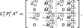  (4.8)

  clearly, $L_{1}^{\sigma } P_{1}^{\sigma } {A^{\sigma }}$ is a complex representation matrix of matrix $\left [ {\begin {array}{*{20}{c}}{\hat {a}_{11}^{(1)}} & {\hat {M}_{12}^{(1)}} \\0 & {\hat {M}_{22}^{(1)}} \end {array}} \right ] + \left [ {\begin {array}{*{20}{c}}{\hat {a}_{11}^{(2)}} & {\hat {M}_{12}^{(2)}} \\0 & {\hat {M}_{22}^{(2)}} \end {array}} \right ]{\text {j}}$, in which $\hat {M}_{12}^{(1)},{\text { }}\hat {M}_{12}^{(2)} \in \textbf {C}^{1 \times (n - 1)},\hat {M}_{22}^{(1)},{\text { }}\hat {M}_{22}^{(2)} \in \textbf {C}^{(m - 1) \times (n - 1)}$ are submatrix after Gauss transformation of matrix M₁, M₂.

After the above step t, M₁, M₂ are two unit upper triangular matrices, i.e.,

(4.9)

For unified representation, P₁,⋯ ,P_r display all exists, P_i(0 ≤ i ≤ r) not all of them exist in the actual operation, and ${\hat {M}^{(1)}}, {\hat {M}^{(2)}} \in \textbf {C}^{r \times n}$ are submatrix after Gauss transformation of matrix M₁, M₂, then the complex representation matrix of the full rank decomposition matrix is

$$ {C^{\sigma} } = \left[ {\begin{array}{*{20}{c}} {{{\hat{M}}^{(1)}}} & {{{\hat{M}}^{(2)}}} \\ { - {{\overline {\hat{M}} }^{(2)}}} & {{{\overline {\hat{M}} }^{(1)}}} \end{array}} \right] \in \textbf{C}^{2r \times 2n},\ B^{\sigma} = {P^{\sigma} }{L^{\sigma} }(:,{\text{ }}[1:r,n:n+r]) \in \textbf{C}^{2m \times 2r}, $$

(4.10)

where $P^{\sigma }=\left (Q_{r}^{\sigma }{\cdots } Q_{2}^{\sigma } P_{1}^{\sigma }\right )^{-1},\ Q_{i}^{\sigma }=\left (L_{i-1}^{\sigma }{\cdots } L_{1}^{\sigma }\right )^{-1}P_{i}^{\sigma }\left (L_{i-1}^{\sigma }{\cdots } L_{1}^{\sigma }\right ),\ 2\leqslant i\leqslant r,\ {L^{\sigma }}=\left (L_{r}^{\sigma } {\cdots } L_{1}^{\sigma } \right )^{- 1}$.

Theorem 4.1

Supposed that A ∈Q^m×n,rank(A) = r, then there exist B^σ ∈C^2m×2r, C^σ ∈C^2r×2n, rank(B^σ) = rank(C^σ) = 2r, satisfies A^σ = B^σC^σ, i.e., A = BC.

By (2.2) and Proposition 2.1, we only need to calculate the first row block of the complex representation matrix in the actual program operation. Next, we give the specific algorithm of the above structure-preserving process.

Example 4.1

For any quaternion matrix $A={A_{1}}+{A_{2}}\mathrm {i}+{A_{3}}\mathrm {j}+{A_{4}}\mathrm {k}\in {{\textbf {Q}}^{m \times n}}$, let m = n = 10 : 10 : 500,A₁ = rand(m, n),A₂ = rand(m, n),A₃ = rand(m, n),A₄ = rand(m, n). Calculate the CPU time and relative error of two algorithms for the full rank decomposition of random quaternion matrices of order 10 to 500 $\left (\eta _{k}=\frac {\left \|{{A_{k}}-{B_{k}}{C_{k}}}\right \|}{\left \|{A}\right \|}\right )$ as follows (Figs. 1 and 2).

Fig. 1

CPU time scatter diagram

Fig. 2

Error scatter diagram of algorithms 1 and 2

Example 4.1 shows that the error of Algorithm 2 is smaller than that of Algorithm 1, and the running time of CPU is also shortened obviously. It can be seen that the result of complex structure-preserving algorithm for the full rank decomposition of quaternion matrices have better timeliness, small error and short running time, which is conducive to the analysis and discussion of a quaternion matrix.

5 A fast algorithm for solving the quaternion linear equations

The main application of the full rank decomposition is to solve the generalized inverse matrix, and then to solve the general solution of corresponding linear equation. At the same time, in the process of the full rank decomposition, we can also get the rank of matrix and so on. In this section, we extend the above two full rank decomposition algorithms, give two algorithms for solving quaternion linear equations, and compare the feasibility and timeliness of the two algorithms. Finally, the complex structure-preserving algorithm of the full rank decomposition is applied to the sparse representation of color images, and the test images are classified.

In addition, the above steps 1–3 is also a fast algorithm for calculating the generalized inverse matrix of quaternion matrix.

Example 5.1

Find the general solution to the system of linear equations Ax = b by the full rank decomposition of matrix A, in which

$$ A=\left[\begin{array}{ccc} 1+2\mathrm{i} & 3\mathrm{j} & 2\mathrm{k}\\ 0 &4+2\mathrm{k} &\text{i+j}\\ 2+4\mathrm{i} &8\text{i+12j}&-3+3\mathrm{k} \end{array}\right],\ b=\left[\begin{array}{ccc} -3+14\text{j+5k} \\ 3+13\text{i+5j+k}\\-29+5\text{i+33j-11k} \end{array}\right]. $$

• (1) By (2.1) and (2.2), we have

  

Run Algorithm 2, and we get

$$ B_{1}=\begin{bmatrix} 1 & 0 \\ 0 & 1 \\ 2 & \mathrm{i} \end{bmatrix},\ B_{2}=\begin{bmatrix} 0 & 0 \\ 0 & 0 \\ 0 & 2 \end{bmatrix},\ C_{1}=\begin{bmatrix} 1+2\mathrm{i} & 0 & 0 \\ 0 & 4 & \mathrm{i} \end{bmatrix},\ C_{2}=\begin{bmatrix} 0 & 3 & 2i \\ 0 & 2\mathrm{i} & 1 \end{bmatrix}, $$

i.e., rand(A) = 2, the full rank decomposition is A = BC, in which

$$ B=\left[ {\begin{array}{*{20}{c}} {\text{1}} & {\text{0}} \\ {\begin{array}{*{20}{c}} {\text{0}} \\ {\text{2}} \end{array}} & {\begin{array}{*{20}{c}} {\text{1}} \\ {{\text{i + 2j}}} \end{array}} \end{array}} \right],{\text{ }}C{\text{ = }}\left[ {\begin{array}{*{20}{c}} {{\text{1 + 2i}}} & {\begin{array}{*{20}{c}} {{\text{3j}}} & {{\text{2k}}} \end{array}} \\ {\text{0}} & {\begin{array}{*{20}{c}} {{\text{4 + 2k}}} & {{\text{i + j}}} \end{array}} \end{array}} \right]. $$

• (2) By (1) and Algorithm 4, it is easy to get

  $$ A^{\dagger}b=\left[\begin{array}{ccc} \text{$-$0.2286+0.4929i+2.8357j$-$1.0286k}\\ \text{ 1.4357+2.0143i$-$0.2429j+0.0929k}\\ \text{ 3.2000+2.4000i+0.1571j+1.2571k} \end{array}\right], $$

then the general solution of linear equations Ax = b is x = A^‡b + (I − A^‡A)y, in which y ∈Qⁿ is any quaternion vector.

Example 5.2

For any quaternion matrix $A={A_{1}}+{A_{2}}\mathrm {i}+{A_{3}}\mathrm {j}+{A_{4}}\mathrm {k}\in {{\textbf {Q}}^{m \times n}}, x={x_{1}}+{x_{2}}\mathrm {i}+{x_{3}}\mathrm {j}+{x_{4}}\mathrm {k}\in {{\textbf {Q}}^{n \times 1}}$, let m = n = 10 : 10 : 500,A₁ = rand(m, n),A₂ = rand(m, n),A₃ = rand(m, n),A₄ = rand(m, n),x₁ = rand(n,1),x₂ = rand(n,1),x₃ = rand(n,1),x₄ = rand(n,1),b = Ax. Calculate the CPU time and relative error of two algorithms for the solution of quaternion linear equations Ax = b of order 10 to 500 $\left (\eta _{k}=\frac {\left \|{A^{\dagger }b-{x}}\right \|_{F}}{\left \|{x}\right \|_{F}}\right )$ as follows (Figs. 3 and 4).

Fig. 3

CPU time scatter diagram

Fig. 4

Error scatter diagram of algorithms 3 and 4

Example 5.2 shows that in terms of calculating the linear equations, the running time and calculation error of Algorithm 4 are also far less than the result of Algorithm 3. And for the calculation of high-dimensional linear equations, Algorithm 3 is difficult to implement, but Algorithm 4 is still fast. In the above chart, in order to compare the results of the two algorithms, we only performed operations within 500 dimensions. In fact, Algorithm 4 can perform higher-dimensional operations.

Example 5.3

Given a color face recognition training data set (Fig. 5), and the corresponding test sample (Figs. 6, 7) are classified. (Color image classification for different subjects. Images of a subject from the Faces95 database.)

Fig. 5

The set of training samples 1, c= 4

Fig. 6

The test sample 1

Fig. 7

The test sample 2

Let A = R i + G j + B k be quaternion representation matrix of the training data set (Fig. 5), b = R_bi + G_bj + B_bk be quaternion representation matrix of the test sample (Figs. 6, 7), where R, R_b, G, G_b, B, B_b are real matrices standing for red, green, and blue colors. A training set is divided into c(c = 4) categories. The goal is exactly to predict the label of b from the given c class training samples. For each class i, let $\delta _{i}: \textbf {R}^{n}\rightarrow \textbf {R}^{n}$ be the characteristic function which selects the coefficients associated with the i th class. The test sample b can be approximated by $\hat {b}_{i}=A\delta _{i}(x)$ which uses the vector δ_i from each class. By using Algorithm 4 and the reconstruction residual for i th class $r_{i}(b)=\| b-\hat {b}_{i} \|_{2}$, we can obtain the approximate sparse representation and classification results of the test image (Figs. 8, 9, 10 and 11).

Fig. 8

The approximate test sample 1

Fig. 9

Figure 6 belongs to the first category of the set of training samples

Fig. 10

The approximate test sample 2

Fig. 11

Figure 7 belongs to the fourth category of the set of training samples

In Example 5.3, four subjects were randomly selected from Faces95 database, and the color face sparse representation was performed on the test images of the first subject and the fourth subject respectively. The results show that the classification is more accurate.

Example 5.4

Given a color face recognition training data set (Fig. 12), and the corresponding test data (Fig. 13) are classified. (Color image classification of different micro expressions of the same subject.) By using Algorithm 4, we can obtain the approximate sparse representation and classification results of the test image (Figs. 14 and 15).

Fig. 12

The set of training samples 2, c= 4

Fig. 13

The test sample 1

Fig. 14

The approximate test sample 1

Fig. 15

Figure 13 belongs to the first category of the set of training samples

In Example 5.4, several sets of micro expression data sets of a subject are randomly selected from the network to sparse represent the different expression images of the same subject. The results show that the classification method is more accurate.

6 Conclusions

In this paper, based on the Gauss elimination method of quaternion matrix, we discuss the direct Gauss transform (based on quaternion toolbox (QTFM) and the complex structure-preserving Gauss transform of a quaternion matrix. By using the Gauss transformation, we obtain the direct algorithm and complex structure-preserving algorithm for the full rank decomposition of a quaternion matrix. Finally, this algorithm can also be applied to the sparse representation classification of color images. The feasibility and timeliness of the proposed algorithms are demonstrated by the corresponding application examples.

References

Adler, S.: Composite leptons quark constructed as triply occupied quasi-particle in quaternionic quantum mechanics. Phys. Lett B. 332, 358–365 (1994)
Adler, S.: Quaternionic Quantum Mechanics and Quantum Fields. Oxford University Press, New York (1995)
De Leo, S., Ducati, G.: Quaternionic groups in physics. Int. J. Theor. Phys. 38, 2197–2220 (1999)
Le Bihan, N., Sangwine, S.: Quaternion principal component analysis of color images. IEEE Int. Conf. Image Process 1, 809–812 (2003)
Mackey, D.S., Mackey, N., Tisseur, F.: Structured tools for structured matrices. Electron. J. Linear Algebra 10, 106–145 (2003)
Sangwine, S., Le Bihan, N.: Quaternion toolbox for matlab. http://qtfm.sourceforge.net/
Jiang, T.: An algorithm for quaternionic linear equations in quaternionic quantum theory. J. Math. Phys. 45(11), 4218–4222 (2004)
Wang, G., Guo, Z., Zhang, D., Jiang, T.: Algebraic techniques for least squares problem over generalized quaternion algebras: A unified approach in quaternionic and split quaternionic theory. Math. Meth. Appl. Sci. 43 (3), 1124–1137 (2020)
Wang, M., Ma, W.: A structure-preserving algorithm for the quaternion Cholesky decomposition. Appl. Math. Comput. 223, 354–361 (2013)
Wang, M., Ma, W.: A structure-preserving method for the quaternion LU decomposition in quaternionic quantum theory. Comput. Phys. Commun. 184(9), 2182–2186 (2013)
Sangwine, S.J.: Comment on ‘A structure-preserving method for the quaternion LU decomposition in quaternionic quantum theory’ by Minghui Wang and Wenhao Ma. Comput. Phys. Commun. 188, 128–130 (2015)
Li, Y., Wei, M., Zhang, F., Zhao, J.: A real structure-preserving method for the quaternion LU decomposition, revisited. Calcolo 54(4), 1553–1563 (2017)
Li, Y., Wei, M., Zhang, F., Zhao, J.: A fast structure-preserving method for computing the singular value decomposition of quaternion matrices. Appl. Math. Comput. 235, 157–167 (2014)
Li, Y., Wei, M., Zhang, F., Zhao, J.: Real structure-preserving algorithms of Householder based transformations for quaternion matrices. Comput. Appl. Math. 305, 82–91 (2016)
Li, Y., Wei, M., Zhang, F., Zhao, J.: On the power method for quaternion right eigenvalue problem. Comput. Appl. Math. 345, 59–69 (2019)
Jia, Z., Wei, M., Ling, S.: A new structure-preserving method for quaternion Hermitian eigenvalue problems. Comput. Appl. Math. 239, 12–24 (2013)
Ma, R., Jia, Z., Bai, Z.: A structure-preserving Jacobi algorithm for quaternion Hermitian eigenvalue problems. Comput. Math. Appl. 75 (3), 809–820 (2018)
Wei, M., Li, Y., Zhang, F., Zhao, J.: Quaternion Matrix Computations. Nova Science Publishers (2018)
Lu, Y., Cui, J., Fang, Z.: Enhancing sparsity via full rank decomposition for robust face recognition. Neural Comput. Appl. 25, 1043–1052 (2014)
Malkoti, A., Vedanti, N., Tiwari, R. K.: A highly efficient implicit finite difference scheme for acoustic wave propagation. J. Appl. Geophys. 161, 204–215 (2019)
Cosnard, M., Marrakchi, M., Robert, Y.: Parallel Gaussian elimination on an MIMD computer. Parallel Comput. 6, 275–296 (1988)
Litvinov, G.L., Maslova, E.V.: Universal numerical algorithms and their software implementation. Program Comput. Software 26(5), 275–280 (2000)
Sheng, X., Chen, G.: Full-rank representation of generalized inverse \(A^{(2)}_{{{TS}}}\) and its application, Comput. Math. Appl. 54, 1422–1430 (2007)
Jiang, M., Jiang, B., Cai, W., Du, X., et al.: Internal model control for structured rank deficient system based on full rank decomposition. Cluster Comput. 20, 13–24 (2017)
Funding
This paper is supported by the Shandong Natural Science Foundation (No. ZR201709250116) and Chinese Government Scholarship (CSC No. 202008370340, No. 202108370086).
Author information
Authors and Affiliations
Corresponding authors
Ethics declarations
Conflict of interest
The authors declare no competing interests.
Additional information
Data availability
All data generated or analyzed during this study are included in this published article (and its supplementary information files).
Publisher’s note
Springer Nature remains neutral with regard to jurisdictional claims in published maps and institutional affiliations.
Rights and permissions
About this article
Cite this article
Wang, G., Zhang, D., Vasiliev, V.I. et al. A complex structure-preserving algorithm for the full rank decomposition of quaternion matrices and its applications. Numer Algor 91, 1461–1481 (2022). https://doi.org/10.1007/s11075-022-01310-1
Received:
Accepted:
Published:
Issue Date:
DOI: https://doi.org/10.1007/s11075-022-01310-1
Keywords
- Quaternion matrix
- Complex representation
- Complex structure-preserving algorithm
- Full rank decomposition
- Sparse representation classification