A patient-specific multibody kinematic model for representation of the scoliotic spine movement in frontal plane of the human body

Abstract

Multibody models of scoliotic spine have shown great promise in planning scoliosis surgery by providing predictive information concerning the surgery outcome. To provide good predictive information, it is important that the kinematic models underlying the movement of the spine models would be personalized to give good estimates of the spine in different positions, which is lacking in the existing literature. This paper aims to develop a patient-specific multibody kinematic model of the scoliotic spine to represent its movement in frontal plane of the human body. The model is an open-chain mechanism comprising rigid links interconnected with rotary joints. To represent the movement, the mechanism lays on the spine curve and estimates the curve and the location and orientation of vertebrae. To personalize the mechanism for a patient, a minimization problem is defined to give the number of the links and their length by using X-rays of different spine positions. The feasibility and capabilities of our patient-specific model are tested by using the data from preoperative X-rays of five positions of 10 AIS (adolescent idiopathic scoliosis) patients; three of the X-rays are routine in scoliosis standard care. The mechanism is personalized to each patient by using the three routine X-rays, and it is used to estimate all the five positions. Root-mean-square-errors (RMSE) of the curve, location, and orientation are 2e–5 mm, 0.27 mm, and 0.25°, respectively. The small RMSEs imply that our kinematic model is capable of estimating the scoliotic spine positions in the frontal plane and thus of describing the scoliotic spine movement in this plane. Our personalization using X-rays of three spine positions helps to set better values for the kinematic parameters (such as the length of the links) for more accurate estimates of the spine in the frontal plane.

1 Introduction

Scoliosis is a complex three-dimensional (3D) structural deformity of the human spine. Surgery is often required to correct the severe deformities [1]. There is no consensus in surgical planning because the scoliosis is a complicated patient-specific deformity [2]. In this regard, biomechanical multibody models of scoliotic spine are effectively helpful in providing predictive information that gives surgeons a rough idea of the surgery outcome [3, 4]. In creating the multibody models of the scoliotic spine, development of patient-specific kinematic models underlying the movement of the models is one of the most important steps [5]. The kinematic models define a joint-link configuration for the spine to define the degree-of-freedom (DOF) of the bodies (e.g. vertebrae and intervertebral discs) and the constraint to their movement [6]. It is important that the kinematic parameters (e.g. the length of the links) of the kinematic models would be personalized for more accurate estimation of the spine. The kinematic models are required to accurately place the vertebrae at their respective location and orientation to better represent the spine positions and, accordingly, the spine movement (considering the movement as the sequence of the positions). Incapability of the kinematic models to represent the spine movement negatively affects the prediction of the surgery outcome [5, 7].

In the existing kinematic models, the spine (including intact and scoliotic) is typically considered as a chain of functional spinal units [8]; a functional unit includes two successive vertebrae and the intervertebral disc [9]. The vertebrae are typically considered as rigid bodies [10, 11]. The intervertebral discs are generally modeled as articulated mechanisms and/or flexible beam elements represented by stiffness matrices. Several studies have considered the intervertebral discs as 3-DOF rotary joints (spherical joint) [12–14]. De Zee et al. [15] and Christophy et al. [8] have placed the center of rotation of the joint on the superior endplate of the lower vertebra of a functional unit. Petit et al. [16] in a study on 82 patients with AIS found that the center of rotation could be at the posterior extremity of the superior endplate. In these models, in a functional unit (Fig. 1a), the spherical joint connects the lower vertebra to the upper one by using a rigid link (the upper vertebra is attached to the link). Figure 1b exemplifies¹ the performance of this mechanism in a real situation. The situation is described by using the X-ray of a functional unit of a scoliotic spine in the frontal plane. As is shown, the mechanism cannot place the upper vertebra (red four-sided shape) on its measured location and orientation (black four-sided shape). The reason for this performance of the mechanism is depicted in Fig. 1c, where the link and joint of the functional unit are placed in their measured location and with their measured orientation. As is clear, there is an offset between the joint and the point $O$ where the link must be connected to the joint. The offset is due to the fact that the stretch of the intervertebral disc is not considered in the mechanism. As such, this mechanism cannot make the possible movement of a vertebra in relation to its adjacent vertebrae. Therefore, the kinematic model that considers the intervertebral disc as a spherical joint may not give a good representation of the scoliotic spine movement. To address the mentioned deficiency, consideration of the intervertebral disc as a beam element can be a viable alternative [17].

Fig. 1

(a) The mechanism of a functional spinal unit comprising the spherical joint, (b) exemplification of the performance of the mechanism, and (c) illustration of the offset

Various studies [18–20] have considered the intervertebral discs as flexible beam elements represented by $6\times 6$ stiffness matrices. Such configuration of the functional units, that is, rigid vertebrae interconnected with flexible beam element, can describe the location and orientation of the vertebrae in 3D space [17, 21]. However, this configuration is not without limitations in representing the scoliotic spine movement. We explain one limitation through an example^∗ of a real situation (Fig. 2). In the example, we make a comparison between the movement directions of the beam element and scoliotic spine in the frontal plane. To represent the movement of the beam element, we consider the movement of its endpoints. The endpoints are the points at which the beam element is attached to its adjacent vertebrae at the middle of the superior and inferior endplates of the vertebrae of a functional unit [3, 22] (Fig. 2a). Figure 2a shows X-rays of a functional unit in the left and right bending positions of a scoliotic spine. The relative location of the endpoints is shown in Fig. 2b in a larger scale for easier illustration. As is clear, the upper endpoint of the beam element in the right bending position (red circle) is in the left side of the upper endpoint in the left bending position (blue circle). Thus, the upper endpoint moved to the left (right) side in the right (left) bending position. In other words, the upper endpoint of the beam element moved to the direction opposite to the direction of the scoliotic spine movement. The opposite movement direction implies that this configuration may not give a good representation of the scoliotic spine movement. The reason is described in the following. The left (right) bending position of the scoliotic spine has been made by exerting a leftward (rightward) force on the spine model in the erect position [23]. The force is applied to the uppermost vertebra of the spine [24]. As is clear in Fig. 2c, the impact of the force, that is, the horizontal component of the force ($F$) and moment ($\tau$), at the upper endpoint (black circle) of the beam element in the erect position must move the endpoint (black circle) to the direction of the bending positions. However, in real situations, the endpoint (black circle) is moved to the direction opposite to the bending direction (blue and red circles). As such, the beam element may not place the upper vertebra of the functional unit on the red/blue four-sided shape representing the measured locations and orientations of the vertebra (Fig. 2a). This shows a mismatch between the simulated bending and the measured scoliotic spine.

Fig. 2

(a) The mechanism of a functional unit comprising the flexible beam element, (b) the relative location of the endpoints of the beam element, and (c) the force and moment applied to the endpoint in the erect position

The existing kinematic models (e.g. [23, 25, 26]) have been typically personalized (e.g. specification of length of links) by minimizing the errors in estimating the location and orientation of the vertebrae of the spine in the erect position. Personalization by using more positions can be helpful to improve the ability of the kinematic models in representation of the spine movement. Such personalization can offer better values for the kinematic parameters (such as the length of the links) for more accurate estimates of the spine curve and the location and orientation of vertebrae in the frontal plane, resulting in better representation of the spine position and thus of the spine movement. However, such a patient-specific kinematic model is considerably lacking in previous studies [5].

The purpose of this paper is to develop a patient-specific kinematic model of the scoliotic spine to represent its movement in the frontal plane. Considering the movement as the sequence of the scoliotic spine positions, the kinematic model represents the movement by describing the positions. In this paper, the positions are described by estimating the scoliotic spine curve and the location and orientation of the vertebrae. We personalize our kinematic model to a patient by using X-rays of a number of spine positions in the frontal plane, whereas the existing kinematic models have been typically personalized by using X-rays of only the erect position. We use X-rays because they are gold standard to describe the spine in a position [27–33]. In this study, we focus on AIS, the most common deformity at adolescents that mostly occurs in female [34].

The paper is organized as follows. Section 2 briefly explains the scoliotic spine and defines the terminologies. In Sect. 3, the problem is defined and formulated. The proposed kinematic model is introduced in Sect. 4. Section 5 evaluates the accuracy of the model. This is followed by a discussion in Sect. 6 on the feasibility and capabilities of the model to represent the scoliotic spine movement. Section 7 concludes the paper.

2 Scoliotic spine

This section briefly describes the scoliotic spine and its evaluation. Scoliosis is a complex 3D structural deformity of the spine affecting between 1.5 % and 3 % of the population [1, 35]. It is defined as a side-to-side curvature of the spine with a twisting of the vertebral column about its axis (Fig. 3a) [36]. This deformity affects the thoracic and lumbar regions of the spine, that is, from the fifth vertebra (L5) of the lumbar region to the first vertebra (T1) of the thoracic region.

Fig. 3

Scoliotic spine in the erect position in the frontal plane: (a) spine regions and (b) Cobb angles

The scoliosis is normally evaluated by measuring Cobb angles on two-dimensional (2D) radiographs [37]. Cobb angles are measured in the frontal plane between the inflection vertebra² and the end vertebrae³ (Fig. 3b) [39]. The severity of the scoliosis is determined by the Cobb angle; the Cobb angle greater than 45° corresponds to the severe scoliosis. Surgical correction is often required for the severe scoliosis.

To describe the geometry of the scoliotic spine in the frontal plane, we define the following terms. The definitions are based on the concept of vertebral body line proposed by Scoliosis Research Society (SRS) (Item #2 in [40]).

• Term 1. Global coordinate system. The system ($G$) is represented by XYZ defined on the lowest vertebra (LV) in the spine model (Figs. 4a and b) and has its origin at the midpoint of the vertebral body of LV (Fig. 4b). The midpoint of a vertebra is the intersection of the line drawn from the upper left corner to the lower right of the vertebral body and the line drawn from the upper right to the lower left of the vertebral body (Fig. 4c shows an example for T9) [38]. The X-axis and Y-axis define the anterior and left directions. The Z-axis is parallel to the line that passes through the center of the upper and lower endplates of LV (an example of the line is shown for T9 in Fig. 4c). The plane YZ is the frontal plane of the human body (Fig. 4b).

  Fig. 4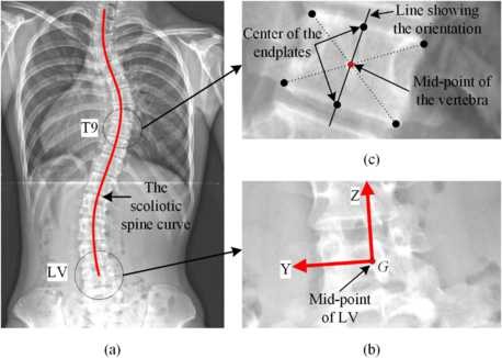

  

  Description of the geometry of the scoliotic spine in the frontal plane: (a) the scoliotic spine curve shown on an X-ray of the scoliotic spine in the erect position, (b) the global coordinate system, (c) the location and orientation of a vertebra

• Term 2. Location of a vertebra. It is the location of the midpoint of the vertebral body in the frontal plane (Fig. 4c).

• Term 3. Orientation of a vertebra. It is the angle between the Z-axis and the line (Fig. 4c) passing through the center of the upper and lower endplates of the vertebra in the frontal plane (Item #27 in [40]).

• Term 4. Scoliotic spine curve. The curve in the frontal plane is the curved line that passes through the midpoints of the vertebral bodies projected on this plane (Fig. 4a) (Item #2 in [40]).

• Term 5. Spinal length. The length in the frontal plane is the arc length of (part of) the spine curve projected on this plane.

• Term 6. Scoliotic spine position. The position in the frontal plane is a term for a configuration of the scoliotic spine in this plane, such as erect (Fig. 4a) and neutral positions.

• Term 7. Scoliotic spine movement. In scoliotic spine movement, the spine starts from a position and ends in another position. The movement is the sequence of the scoliotic spine curves representing the first, intermediate, and last positions of the spine in the context of this paper.

3 Problem definition

Despite recent attempts made to classify the scoliotic deformity by using 3D classification [41], to the best of our knowledge, there is no consensus in interpretation of 3D classification and validation for the surgical treatment guidelines. The current standard care for surgical treatment of 3D scoliotic deformity relies heavily on the use of 2D radiographs taken in the frontal plane [42, 43]. In planning the surgery, the spinal flexibility in the frontal plane is one of the key parameters to identify the correct spinal fusion levels and the extent of spinal instrumentation required to correct the scoliotic deformity [2, 23]. The flexibility is the difference of spinal excursion (movement) from the erect to lateral bending positions [42]. Various clinical tests have been made to assess the spinal flexibility since the onset of scoliosis surgical correction [2]. These include 2D radiographs of the spine in the erect position and 2D radiographs of the lateral bending positions [44], 2D fulcrum bending radiographs [45], 2D supine traction [46], and/or 2D push prone radiographs [47]. Moreover, in evaluating the outcome of scoliosis surgical correction, one of the main parameters is the straightness of the spine curve in the frontal plane [1]. To measure the straightness, the Cobb angles are measured on post-operative 2D radiograph of the erect spine. Therefore, these parameters from the scoliotic spine in the frontal plane are of primary importance in planning and evaluation of the scoliosis surgical correction. By using analytical methods these parameters, important for surgery planning and evaluation, can be measured on the spine curves provided by the simulated spines [40, 48, 49]. As such, in order that multibody models of the scoliotic spine be of great help in surgery planning, it is essential that the kinematic models offer good estimates of the spine curve in the frontal plane. One crucial step in this regard is to personalize the kinematic parameters (such as the length of the links) to a given patient for more accurate estimation of the patient’s spine curves [5]. Overall, for “surgical correction prediction” application, we found it more proper to develop a 2D multibody kinematic model of the scoliotic spine whose kinematic parameters are personalized by using X-rays of a number of spine positions to give good estimates of the spine curve in the frontal plane.

This section formulates the problem of 2D kinematic modeling of the scoliotic spine and describes the input, the output, and the relationships between the input and output.

3.1 Input: the scoliotic spine curve

The scoliotic spine curve projected on the frontal plane is the input of our model. To obtain the curve, X-rays are used because they are considered as the gold standard in the spine modelling and validation [27–29].

The curve in the frontal plane (YZ, Fig. 4b) is a mathematical function $f$ of Z. The curve of position $i$ is given by $\mathrm{Y}=f_{i}$(Z), $i=0,1,\ldots ,\infty$. The zero position (the reference position in this paper) corresponds to the posterior–anterior erect position (or simply erect position) of the scoliotic spine. We consider the erect position as the reference because it is the reference position for the scoliosis evaluation and its surgical correction planning. Besides, the X-ray taken from the spine in the erect position is a part of the standard care for monitoring scoliosis [29].

The locations of the vertebrae in a position are defined by the ordered pairs of (Y, Z). The orientations of the vertebrae are given by the first derivative of $f$ at the location of the vertebrae, that is, $\lambda_{j} =df(\mathrm{Z})/d\mathrm{Z}$ at $\mathrm{Z}_{j}$, where $j$ denotes the $j$th vertebra. Since $G$ has its origin at the midpoint of LV in all positions, the location of LV is $(\mathrm{Y}_{1},\mathrm{Z}_{1})=(0,0)$. The orientation of LV is $\lambda_{1} =f'(0)=0$ since the line showing its orientation is the Z-axis of $G$.

3.2 Output: the patient-specific kinematic model

The output is the kinematic model of the scoliotic spine of a patient in the frontal plane. The kinematic model is an open-chain mechanism that lays on the scoliotic spine curve. To characterize the mechanism, a multibody configuration of the joints and links is to be defined. The mechanism has $n$ 1-DOF rotary joints.

The mechanism in each position estimates the scoliotic spine curve and the location and orientation of the vertebrae. ($\mathrm{Y}^{*}_{j},\mathrm{Z}^{*} _{j}$) and $\lambda^{*}_{j}$ give the estimated locations and orientations of the $j$th vertebra, respectively. The estimated curve is the curve fitted to these estimates, and it is represented by $\mathrm{Y}^{*} =f^{*}_{i}$(Z) for position $i$.

3.3 Problem formulation

To represent the scoliotic spine movement in the frontal plane, the kinematic model should be capable of representing the scoliotic spine positions. In this regard, the model is required to estimate the scoliotic spine curve and the location and orientation of the vertebrae in the positions. Three criteria (1) are defined to determine the accuracy of the estimates: RMSE between the scoliotic spine curve and its estimate and RMSE between the locations/orientations of the vertebrae and their estimates.

$$ \left\{ \begin{aligned} &\mathrm{RMSE}\ \mbox{of the curve} = \sqrt{ \frac{1}{Q} \sum_{q=1}^{Q} \bigl( f_{i}^{*} ( \mathrm{Z}_{q} ) - f_{i} ( \mathrm{Z}_{q} ) \bigr) ^{2}}, \\ &\mathrm{RMSE}\ \mbox{of the location}= \sqrt{ \frac{1}{k} \sum_{j =1}^{k} \left( \left( \mathrm{Y}_{j}^{*} - \mathrm{Y}_{j} \right) ^{2} + \left( \mathrm{Z}_{j}^{*} - \mathrm{Z} _{j} \right) ^{2} \right) ,} \\ &\mathrm{RMSE}\ \mbox{of the orientation}= \sqrt{ \frac{1}{k} \sum_{j =1}^{k} \left( \lambda_{j}^{*} - \lambda_{j} \right) ^{2}}, \end{aligned} \right. $$

(1)

where $Q$ is the total number of data points ($\mathrm{Y}^{*},\mathrm{Z}$) considered on the estimated curve to be compared with the data points (Y, Z) on the curve, ($\mathrm{Y}_{1},\mathrm{Z}_{1}$) and ($\mathrm{Y}_{Q},\mathrm{Z}_{Q}$) are the locations of LV and the uppermost vertebra in the model, respectively, and $k$ is the total number of the vertebrae in the model.

4 Description of the kinematic model

4.1 Assumption

To develop the model, we make the following assumption: “the change in the spinal length (Term 5, Sect. 2) from L4 to T2 is negligible during the movement.” The assumption indicates that the spinal lengths ($L$) of all the positions are equal, that is, $L_{0} =L_{1} =\cdots =L _{\infty }$. In this paper, the assumption is considered valid if $|L_{0} -L_{i}|$ for $i=1,2,\ldots ,\infty$ is less than 0.5 % of $L_{0}$, where $|\boldsymbol{\cdot }|$ denotes the absolute operation. The assumption and the constraint (0.5 %) will be supported in Sect. 5.5.

4.2 Configuration of the model

In the context of mathematics, a curve can be approximated by a piecewise linear curve consisting of a number of straight lines of equal length. In relation to this statement, two curves of equal length can be approximated by the same number of the lines if the length of the lines is sufficiently small. The Appendix briefly explains the approximation and the term sufficiently small lines. Therefore, referring to the assumption, the scoliotic spine curves in different positions can be approximated by the same number ($n$) of the sufficiently small lines. Thus, we define the kinematic model as a chain of $n$ rotary segments. A rotary segment (Fig. 5a) consists of a rigid straight link (corresponding to the straight lines) and a 1-DOF rotary joint (corresponding to the connecting points of the successive lines). The links of the rotary segments are equal in length ($L_{ \mathrm{seg}}$ in the Appendix). The chain lays on the scoliotic spine curve to estimate the curve (Fig. 5b). The chain is constrained at the first rotary segment attached to the midpoint of LV. The first rotary segment cannot translate with respect to the midpoint of LV. The last rotary segment corresponds to the midpoint of the uppermost vertebrae. The kinematic model is characterized by $n$ rotary segments if $L_{\mathrm{seg}}$ is sufficiently small. In Sect. 4.3, we specify the term sufficiently small and explain how $L_{\mathrm{seg}}$ and $n$ are obtained.

Fig. 5

The configuration of the proposed kinematic model and the coordinate systems: (a) a rotary segment and its location and orientation defined in $G$ and (b) the chain of rotary segments laid on the spine curve

We adopt the Denavit–Hartenberg (DH) convention [50] to represent the chain. The coordinate systems in Fig. 5 are attached according to the DH convention. The rotation axes of the joints are parallel to each other and perpendicular to the frontal plane. The location of a rotary segment is the location of the origin of its coordinate system ($xy$ in Fig. 5a) in $G$. The orientation of the rotary segment is the orientation of the $x$-axis of its coordinate system with respect to the Z-axis of $G$.

Table 1 illustrates the DH parameters [50]. The first two rows of Table 1 are for transformation of $G$ to the coordinate system $x_{0} y_{0} z_{0}$. Referring to the configuration of the model, the offsets along the previous $z$ to the common normal ($d$) are zero, and the angles about the common normal ($\alpha$) are zero for transformation of the coordinate system of a rotary segment to the next one. The scoliotic spine positions are defined by specifying $\theta_{1}$ to $\theta_{n}$.

Table 1 The DH parameters

4.3 Personalization of the model

The model is personalized by specifying $n$ and $L_{\mathrm{seg}}$. As the chain represents the spine curve, the length of the chain ($n \cdot L_{\mathrm{seg}}$) should estimate the spinal length in all the positions. We consider that the acceptable estimation error (i.e. $|L_{0} -n_{i} \cdot L_{\mathrm{seg}}|$) is less than 0.5 % of $L_{0}$ according to the assumption. Besides, $L_{\mathrm{seg}}$ should be sufficiently small to result in the same number of rotary segments in all the positions, i.e. $n_{0} =n_{1} =\cdots =n_{\infty }$. It should be noted that $n_{i}$ may be different due to the differences $|L_{0} -L_{i}|$. Therefore, to find a sufficiently small $L_{ \mathrm{seg}}$, the linear programing problem (or simply the minimization problem) in (2) is defined. The minimization problem finds $L_{\mathrm{seg}}$ and $n_{i}$ such that $\sum |n_{0} -n_{i}|$ is minimized. Each $L_{\mathrm{seg}}$ on the spine curve of position $i$ gives an $n_{i}$. After solving the minimization problem, a sufficiently small $L_{\mathrm{seg}}$ is obtained, and $n$ is the number of segments obtained for the erect position ($n_{0}$).

$$ \textstyle\begin{array}{c@{\quad }c} \min \left\vert n_{0} - n_{1} \right\vert + \left\vert n_{0} - n_{2} \right\vert + \cdots + \left\vert n_{0} - n_{\infty } \right\vert & \\ \text{subject to constraints} & \left\vert L_{0} - n_{0} \boldsymbol{\cdot } L_{\mathrm{seg}} \right\vert < 0.005 L_{0} \\ & \left\vert L_{0} - n_{1} \boldsymbol{\cdot } L_{\mathrm{seg}} \right\vert < 0.005 L_{0} \\ & \vdots \\ & \left\vert L_{0} - n_{\infty } \boldsymbol{\cdot } L_{\mathrm{seg}} \right\vert < 0.005 L_{0} \end{array} $$

(2)

After personalization of the model, the rotary segments with the location closest (Euclidean distance) to the location of the vertebrae are specified on the chain in the erect position. The location and orientation of these rotary segments, labeled by $s$, are the estimates of the location and orientation of the vertebrae in all the positions. The estimated locations ($\mathrm{Y} ^{*}_{j}$, $\mathrm{Z}^{*}_{j}$) and orientations $\lambda^{*}_{j}$ of the $j$th vertebra are given by the locations and orientations of $s_{j}$, respectively.

5 Proof-of-concept

The feasibility and capability of the proposed kinematic model are shown by representing the spine movement of our cohort of 10 patients. The accuracy of the model in representing the spine movement is tested. The assumption is also tested.

5.1 Materials and data acquisition

After obtaining domain-specific review board approval, preoperative X-rays of 10 patients with AIS were used for the study. The X-rays were taken in five posterior–anterior positions in the frontal plane, one erect position and four prone positions: left bending, right bending, neutral, and traction positions that are the positions 1, 2, 3, and 4, respectively. The patients had no neurological deterioration, and they were admitted to hospital for surgical treatment. Table 2 illustrates descriptive data of the patients. There were eight female and two male patients with age ranging from 13 to 19 years (mean age of 15 years); LV and the uppermost vertebra in this study were L4 and T2. It should be noted that L5 and T1 were excluded since the X-rays at these vertebrae were often suboptimal for the measurement. $L_{0}$ was calculated from L4 to T2 and tabulated in Table 2. The average and median Cobb angles of the main curves were 52° and 53°, respectively.

Table 2 Descriptive data of the patients

The preoperative X-rays were analyzed to extract the location and orientation of the vertebrae from L4 to T2. The limit of accuracy ($\delta$) of measurements of the locations was 0.1 mm, and that ($\Delta$) of the orientations was 0.1°. The orientations were obtained by utilizing the tangent formula. To do this, the line showing the orientation of the vertebra (Fig. 4c) and Z-axis of $G$ were considered as the hypotenuse and cathetus (B) of a right triangle, respectively (Fig. 6a). The length of B was considered 100 mm. Thus, by measuring the length of the other cathetus (A), the orientation is given by $\tan^{-1}$ (A/100). The $\delta$ of measurements of A and B was 0.1 mm. As such, $\Delta$ is given by (3). The greatest $\Delta$ was almost 0.07° (Fig. 6b). Thus, $\Delta$ was considered 0.1°. It should be noted that the largest measured A was around 60 mm.

$$ \Delta = \max \left( \left\vert \tan^{-1} \left( \frac{\mathrm{A} \pm \delta }{\mathrm{B}\pm \delta } \right) - \tan^{-1} \left( \frac{ \mathrm{A}}{100} \right) \right\vert \right) . $$

(3)

Two experts familiar with spine X-rays manually performed the measurements three times. Then, the mean values of the measurements were considered for this study. All the measurements were supervised by G. Liu, who is an experienced scoliosis surgeon working at National University Hospital, Singapore. The intra- and inter-observer reliabilities of the measurements were evaluated by using Pearson correlation analysis. The intra-observer correlation coefficients were $0.95\pm 0.04$ for expert 1 and $0.92\pm 0.03$ for expert 2. These agreements are excellent according to [51] and can demonstrate the repeatability of the measurements. The inter-observer coefficient was 0.90. Overall, the strong correlations indicate the repeatability and reliability of the measurements.

Fig. 6

(a) Measurement of the orientation of the vertebrae and (b) the limit of accuracy of the orientation against the measured A

5.2 The scoliotic spine curve representation

To represent the spine curve, a polynomial was fitted to the measured location and orientation of the vertebrae by using the linear least squares method. The order of the polynomials was adjusted to find the best fitting, that is, the least RMSE of the locations and orientations.

The curves ($f$) are estimated by the polynomial in (4); $f$ has no first-degree and constant terms because $f(0)=0$ and $f '(0)=0$ (Sect. 3.1). Equation (5) gives the coefficients of $f$ in terms of the measured parameters. $\boldsymbol{\beta }$ and $\mathbf{Y}$ are the vectors of the coefficients and measured parameters, respectively, and $\mathbf{Z}$ is the design matrix. Equation (6) gives $\boldsymbol{\beta }$, $\mathbf{Z}$, and $\mathbf{Y}$. The upper and lower halves of $\mathbf{Y}$ and $\mathbf{Z}$ correspond to the measured locations and orientations, respectively.

$$ f \left( \mathrm{Z} \right) = \beta_{t} \mathrm{Z}^{t} + \beta_{t -1} \mathrm{Z}^{t-1} +\cdots + \beta_{2} \mathrm{Z}^{2}, $$

(4)

where $\beta_{t},\ldots ,\beta_{2}$ are the coefficients, and $t$ is the order of the polynomial.

$$ \boldsymbol{\beta } = \left( \mathbf{Z}^{\mathrm{T}} \mathbf{Z} \right) ^{-1} \mathbf{Z}^{\mathrm{T}} \mathbf{Y}, $$

(5)

where ^T sign stands for transpose operation.

$$\begin{aligned} &\textstyle\begin{array}{c@{\qquad }c} \boldsymbol{\beta } = \left[ \textstyle\begin{array}{c} \beta_{t} \\ \beta_{t -1} \\ \vdots \\ \beta_{2} \end{array}\displaystyle \right] & \mathbf{Z} = \left[ \textstyle\begin{array}{c@{\quad }c@{\quad }c@{\quad }c} \textstyle\begin{array}{c@{\quad }c@{\quad }c@{\quad }c} \mathrm{Z}_{1}^{t} & \mathrm{Z}_{1}^{t -1} & \cdots & \mathrm{Z}_{1} ^{2} \\ \mathrm{Z}_{2}^{t} & \mathrm{Z}_{2}^{t -1} & \cdots & \mathrm{Z}_{2} ^{2} \\ \vdots & \vdots & \ddots & \vdots \\ \mathrm{Z}_{k}^{t} & \mathrm{Z}_{k}^{t -1} & \cdots & \mathrm{Z}_{k} ^{2} \end{array}\displaystyle & \\ & \\ \textstyle\begin{array}{c@{\quad }c@{\quad }c@{\quad }c@{\quad }c} t \mathrm{Z}_{1}^{t -1} & \left( t-1 \right) \mathrm{Z}_{1}^{t -2} & \cdots & & 2 \mathrm{Z}_{1}^{1} \\ t \mathrm{Z}_{2}^{t -1} & \left( t-1 \right) \mathrm{Z}_{1}^{t -2} & \cdots & & 2 \mathrm{Z}_{2}^{1} \\ \vdots & \vdots & \ddots & & \vdots \\ t \mathrm{Z}_{k}^{t -1} & \left( t-1 \right) \mathrm{Z}_{k}^{t -2} & \cdots & & 2 \mathrm{Z}_{k}^{1} \end{array}\displaystyle & \end{array}\displaystyle \right] \textstyle\begin{array}{c} \left. \textstyle\begin{array}{c} \\ \\ \\ \\ \end{array}\displaystyle \right\} \textstyle\begin{array}{c} \mathrm{The} \\ \mathrm{Upper} \\ \mathrm{Half} \end{array}\displaystyle \\ \\ \left. \textstyle\begin{array}{c} \\ \\ \\ \\ \end{array}\displaystyle \right\} \textstyle\begin{array}{c} \mathrm{The} \\ \mathrm{Lower} \\ \mathrm{Half} \end{array}\displaystyle \end{array}\displaystyle \end{array}\displaystyle \\ &\textstyle\begin{array}{ll} \mathbf{Y} = &\left[ \textstyle\begin{array}{c} \textstyle\begin{array}{c} \mathrm{Y}_{1} \\ \mathrm{Y}_{2} \\ \vdots \\ \mathrm{Y}_{k} \end{array}\displaystyle \\ \\ \textstyle\begin{array}{c} \tan \lambda_{1} \\ \tan \lambda_{2} \\ \vdots \\ \tan \lambda_{k} \end{array}\displaystyle \end{array}\displaystyle \right] \textstyle\begin{array}{c} \left. \textstyle\begin{array}{c} \\ \\ \\ \\ \end{array}\displaystyle \right\} \textstyle\begin{array}{c} \mathrm{The} \\ \mathrm{Upper} \\ \mathrm{Half} \end{array}\displaystyle \\ \left. \textstyle\begin{array}{c} \\ \\ \\ \\ \end{array}\displaystyle \right\} \textstyle\begin{array}{c} \mathrm{The} \\ \mathrm{Lower} \\ \mathrm{Half} \end{array}\displaystyle \end{array}\displaystyle \end{array}\displaystyle , \end{aligned}$$

(6)

where $k =15$ in this study.

Table 3 shows the order $t$ and RMSE of the locations and orientations for each patient. RMSE calculated for the locations was $0.19\pm 0.10\mbox{ mm}$ and for the orientations was 0.16 ± 0.07°. The small RMSEs show that the fitted polynomials can give good estimates of the locations and orientations of the vertebrae.

Table 3 The data of polynomials, including the orders and the fitting errors

5.3 Kinematic models for the individual patients

Before solving the minimization problem, first, we tested whether the spinal lengths of the individual patients satisfied the assumption in Sect. 4.1. The difference between the lengths in the erect and other positions ($E_{i} =100\times (L_{0} -L_{i})/L_{0}$) was in the range of $[-0.27,0.31]$ for all the patients (Table 4); $E_{i} =\pm 0.5\mbox{ \%}$ corresponds to the marginal acceptable $L_{0} -L_{i}$. As such, the assumption $|L_{0} -L_{i} |<0.005L_{0}$ is satisfied for all the patients. Therefore, for each patient, there exists an $L_{\mathrm{seg}}$ that satisfies the constraints in the minimization problem (2). Therefore, the model is personalized in the following.

Table 4 The change in the length of the scoliotic spine curves with respect to $L_{0}$

The kinematic model was personalized by using the curves of three positions: erect, left bending, and right bending. These three positions were chosen because their X-rays are routinely taken for the scoliosis monitoring and the surgical correction planning. Then, using the personalized models, we estimated the spine curves of all the five positions. This was done to evaluate the feasibility and capability of our kinematic model in representing the scoliotic spine movement (will be discussed in detail in Sect. 6).

To personalize, $L_{\mathrm{seg}}$ and $n$ were computed by solving the minimization problem (2). To solve (2), the spinal lengths of the three positions (erect, left bending, and right bending) were used. For each $L_{\mathrm{seg}}$ satisfying the constraints (i.e. $|L_{0} -n_{i} \times L_{\mathrm{seg}} |<0.005L_{0}$; note that $n_{i}$ is the round of $L_{i} /L_{\mathrm{seg}}$ to the nearest integer), the chain was laid on $f_{0}$, $f_{1}$, and $f_{2}$ to obtain $n_{0}$, $n_{1}$, and $n_{2}$ respectively. After that, $L_{\mathrm{seg}}$ was chosen the one that minimizes $|n_{0} -n_{1} |+|n_{0} -n_{2}|$, and $n$ obtained for the erect position (i.e. $n_{0}$) was considered for the model. After personalization of the model, $s_{j}$ for $j=1,2,\ldots ,15$ were found in the erect position (position 0). In our patient cohort, $n$ ranged from 994 to 1003 ($999\pm 3$), and $L_{\mathrm{seg}}$ was between 0.32 and 0.44 mm ($0.37\pm 0.04\mbox{ mm}$). The estimation error of the spinal length ($e_{i} =L_{i} -n_{0} \cdot L_{\mathrm{seg}}$) for the positions included in the personalization (positions 0, 1, and 2) was $0.28\pm 0.40\mbox{ mm}$, and $e$ was $0.13\pm 0.44\mbox{ mm}$ for the other two positions. These small errors show that the mechanism can estimate the spinal length in the frontal plane. The error $e$ will be discussed in detail in Sect. 6.

5.4 Accuracy of the model

To compute the accuracy, first, the personalized model was laid on the spine curves of the five positions (Fig. 7). Second, ($\mathrm{Y}^{*},\mathrm{Z} ^{*}$) and $\lambda^{*}$ were determined for the 15 vertebrae. RMSE of the location and orientation were calculated by (1). Third, RMSE of the curve was calculated between $f$ and the curve estimated by the model ($f^{*}$) by (1); $f^{*}$ was obtained by considering the chain as a continuous piecewise function of Z. To do this, the joints of the chain were considered as points on $f^{*}$, and their intermediate points were interpolated by using straight lines connecting the joints.

Fig. 7

Representation of the scoliotic spine curve by the proposed kinematic model (this figure is only for the illustration purpose and does not represent a real situation in terms of shape of the spine curve and location and orientation of a vertebra with respect to its inferior one)

For the three positions included in the personalization, RMSEs of the locations and orientations are 0.30 mm and 0.25° respectively (Table 5). For the two positions not included in the personalization, the RMSEs are 0.23 mm and 0.24°, respectively. RMSE of the curves (for both cases) is 3e–5 mm. As is clear, RMSEs are quite small for the locations and orientations, and particularly for the curves. The small RMSEs imply that the model can accurately estimate the scoliotic spine curve and the location and orientation of its vertebrae not only in the three positions used for the personalization but also in the other two positions. As such, our patient-specific kinematic model can give good estimates of the spine positions. Besides, the proposed personalization method can offer good personalization of our kinematic model by using a few positions. Figure 8 shows an example of the chain in the five positions for one of the patients. A visual comparison shows that the curves, locations, and orientations estimated by the chain agree well with the measured ones. Overall, it can be concluded that our kinematic model is feasible and capable of representing the scoliotic spine positions and thus of describing the scoliotic spine movement in the frontal plane. The feasibility and the capability will be discussed in detail in Sect. 6.

Fig. 8

(a) the measured scoliotic spine positions, (b) the estimated scoliotic spine positions by the proposed kinematic model

Table 5 RMSE obtained for the scoliotic spine curves and the location and orientation of the vertebrae

5.5 Support of the assumption

To support the assumption (Sect. 4.1), statistical analysis was performed on the data of the change in the spinal length from L4 to T2 (E, Table 4) and RMSEs of the spine curve and the location and orientation of the vertebrae (Table 5). The results of the statistical analysis are depicted by box charts (Fig. 9). Shapiro–Wilk’s test [52] showed that the data of $E$ were significantly drawn from a normally distributed population $N_{E}$ ($\mathrm{mean}=-0.02, SD^{2} =0.13^{2}$) at 1 % significance level. In addition, Anderson–Darling’s test [53] demonstrated that the data of the RMSEs (the red, blue, and magenta charts) could be described by the gamma distribution $\Gamma$ (shape, scale) at 1 % significance level. According to the distribution functions and with 99 % confidence interval, $E$ is between −0.36 and 0.32 mm, and such change in the spinal length causes RMSEs less than 6e–5 mm, 0.52 mm, and 0.53° for the spine curve and the location and orientation of the vertebrae, respectively. These small RMSEs show that the proposed kinematic model can give good estimates the spine positions, even though the spinal length is changed by 0.36 %. Therefore, the assumption, underlying neglecting the change in the spinal length, can be valid for representing the scoliotic spine movement in the frontal by the proposed patient-specific kinematic model.

Fig. 9

The box charts of the data

The reasons for considering the coefficient 0.5 % for neglecting $E$ and for the constraints in the minimization problem (2) are explained as follows. First, from $N_{E}$ it was found that the chance of getting $|E|<0.5\mbox{ \%}$ was around 99.99 %, which is quite high. Besides, it was shown that $E$ drawn from $N_{E}$ (Fig. 9) caused small RMSEs in representing the spine curve and location and orientation of the vertebrae. Therefore, we considered the change of less than 0.5 % in the spinal length as a negligible change. Second, for the minimization problem, on the one hand, it is important that the coefficient of $L_{0}$ be large enough so that all the constraints are satisfied. On the other hand, it is important that the coefficient value be small to reduce the computational expense incurred by the minimization problem (note that increase in the value exponentially increases the computational expense). The coefficient value of 0.5 % could make a trade-off between these conflicting conditions. It was considered as the smallest value for the remarkable chance (99.99 %) of satisfying all the constraints in (2).

5.6 Representation of the lateral bending movement of the scoliotic spine

The developed kinematic model represents the scoliotic spine movement by the trajectory of its joint variables ($\theta$). The amount of rotation ($\Delta \theta$) of the joints with respect to the neutral position was calculated for the left and right bending positions for all the patients (Table 6). The neutral position was used as the substitute for the erect position because the neutral, left bending, and right bending X-rays were taken in the same laying position (prone), whereas the erect was a stand-up position. Therefore, we found it more proper to use neutral X-ray for the assessment of the performance of the model. The results in Table 6 show that more than 98 % of the total amount of the rotation occurs toward the direction of the bending (i.e. toward the horizontal component of the applied force for making the bending movements). This means that our model is able to give good estimates of the lateral bending positions when the force is applied toward the direction of the bending.

Table 6 The amount of the rotation of the joints in the left and right bending positions

Figure 10 shows an example done for a patient. $\Delta \theta$ is shown by a 2D area drawn with respect to the spine curve in the left and right bending positions. The curves of the positions were considered as the reference lines for the direction of the rotation, that is, $\Delta \theta$ in the left (right) side of the reference curve means the amount of the rotation toward the left (right) side. The blue and magenta colors correspond to the amount of the rotation of the rotary segments between two successive vertebrae. The area of $\Delta \theta$ between two successive vertebrae is the amount of the rotation of the superior vertebra with respect to its inferior one. Furthermore, the area of $\Delta \theta$ is the amount of the rotation of T2 with respect to L4. As can be seen, almost the total amount of the rotation is toward the direction of the bending except the quite small area in the left bending position.

Fig. 10

$\Delta \theta$ in the lateral bending positions

6 Discussion

To demonstrate the feasibility and capability of the proposed patient-specific kinematic model, first, the model was personalized by using three routine X-rays taken in the erect and lateral bending positions, and the personalized models were used to represent the spine in two other positions and in the three positions. It was shown that the model could give good estimates of the spine curves and the locations and orientations of the vertebrae in all the positions. Besides, the assumption made to develop the kinematic model was also supported by performing statistical analysis on the estimation errors. The minimization problem (2) was proposed to personalize the values of the kinematic parameters by using X-rays of several spine positions. This distinguishes our patient-specific kinematic model from the existing ones, whose kinematic parameters are typically obtained by using X-rays of only erect position. Involving X-rays of more spine positions helps setting better values of the kinematic parameters for more accurate estimates of the spine positions.

The feasibility of the proposed kinematic model traces back to the minimization problem (2). The minimization problem has a solution for the “sufficiently small” length for a given patient if and only if the area limited to the constraints is not null. In Sect. 5.5, through statistical analysis, it was shown that at 99.99 % confidence interval, the change in the spinal length is less than 0.5 % of the length of the erect spine. This can confirm that at least one $L_{\mathrm{seg}}$ exists to specify an $n$ for all the spine positions of a given patient, and thus the model can be feasible. Moreover, in practice, only a few positions are available to solve the minimization problem. Thus, to have a more complete examination of the feasibility, we need to show that “the model that is personalized by a few positions can give good estimates of all the spine positions.” In this regard, we performed the personalization by using X-rays of three positions, and then we showed that the personalized models could accurately estimate the other two positions not included in the personalization as well as the three positions. Besides, the X-rays of the three positions are routine in scoliosis standard care. Therefore, our model personalized by using the routine X-rays has the potential to represent the scoliotic spine movement. Overall, it can be concluded that the developed kinematic model is feasible.

The capability of the model for representing the scoliotic spine movement was demonstrated by testing the accuracy of the model in estimation of the five positions. RMSE of 50 curves was not significant (less than 6e–5 mm), and RMSEs of the location and orientation of 750 vertebrae were less than 0.59 mm and 0.38°, respectively (Table 5). These small RMSEs for the five positions can show that our model can accurately estimate the spine positions. Therefore, the model can be capable of representing the scoliotic spine movement by estimating a sequence of the spine positions. In addition, the small RMSEs of the locations and orientations imply that the rotary segments $s$ can be accurate estimates of the vertebrae in terms of their locations and orientations.

In general, a 2D spine model in the frontal plane does not include the information relating to the torsion, kyphosis, and lordosis angles of the spine. This can have negative effects on the accuracy of the 2D model in estimating the parameters such as the curvature angle (measured by the analytic Cobb method) [40] and spinal flexibility and mobility. These are the key parameters measured in the frontal plane for surgical planning [23]. To measure/calculate the parameters by using analytic methods [48, 49, 54], the first derivative of the spine curve is required. It was demonstrated that the proposed model estimated the curve with small RMSE of 3e–5 mm (Table 5), showing that the shape of the curve is preserved. Besides, the small RMSEs of the orientations of the vertebrae (0.25°, Table 5) show that the first derivatives of the estimated curves at the midpoints of the vertebrae were good estimates of those on the measured curves. Therefore, it can be concluded that the first derivative of the estimated curves can correspond well with the first derivative of the measured curves. Overall, the proposed model is able to give good estimates of the key parameters without taking into consideration the torsion, kyphosis, and lordosis angles.

The proposed kinematic model neglects the change in the spinal length and considers the links as rigid bodies according to the assumption. It was demonstrated that these concepts could not significantly influence the accuracy of the kinematic model. In the following, we discuss that the concepts may also not raise major issues in a dynamic model that is based on the developed kinematic model. Regarding the concept of neglecting the length change, it was shown that the model could estimate the spinal length with the error $e=0.22\pm 0.43\mbox{ mm}$ in Sect. 5.3; $e$ is the sum of two errors, namely $ec$ and $em$. The former is the error of approximating parts of the curve with straight lines (Fig. 11a), and $ec$ is the sum of differences between $L_{\mathrm{part}}$ and $L_{\mathrm{seg}}$ from L4 to T2, and it is always positive. $ec$ was $0.21\pm 0.18\mbox{ mm}$, and the differences ($L_{\mathrm{part}} -L_{ \mathrm{seg}}$) were 2e–$4\pm 2$e–4 mm. Such small differences from L4 to T2 can show that the rotary segments correspond to their associated spine parts. Thus, $ec$ may not significantly affect the accuracy of the dynamic model that is based on the proposed kinematic model. The second error ($em$) is the distance between the locations of the midpoint of T2 and the last rotary segment; $em$ is negative (Fig. 11a) when the last rotary segment adds extra length to the curve; otherwise, it is positive (Fig. 11b). $em$ was $0.02\pm 0.26\mbox{ mm}$. Studies that model the spine joints as 3D spherical joints (see Introduction) neglect the change in the spinal length and accordingly $ec$ and $em$ in their kinematic models. The errors $ec$ and $em$ in these models can be greater than the errors in our model because the models approximate much larger parts (functional units) of the spine with rigid links in comparison with our model. Neglecting such larger errors has had no significant effect on the accuracy of the dynamic models [8, 15, 23]. As such, our kinematic model with such smaller errors may not raise major issues in dynamic modeling. The concept of rigidity of the links was formulated according to studies of Panjabi et al. [18] and Oxland et al. [55] on the stiffness of the thoracic and thoracolumbar spine, respectively. They found that the stiffness in the axial direction is high, and thus, the impact of this stiffness on the dynamics is negligible, showing that the assumption of the rigid links may not raise major issues in dynamic modeling as well. As a future work, we are in the process of creating a patient-specific multibody dynamic model of the scoliotic spine by utilizing the developed kinematic model.

Fig. 11

Illustration of $ec$ and $em$: (a) $em<0$ and (b) $em>0$

The developed patient-specific kinematic model represents the scoliotic spine curve by the chain of small rotary segments ($0.37\pm 0.04\mbox{ mm}$ in our sample). The model is well suited to do the in-depth analysis of the kinematics of the scoliotic spine in the frontal plane, as the model provides the changes of the spine curve during the spine movement [56, 57]. This analysis can help to improve the knowledge of the scoliotic spine movement before surgery, which is considerably limited in the literature [29, 57]. Such knowledge is important for the preoperative planning of scoliosis surgery [43, 58]. The proposed model can provide useful information about intriguing relationships between the flexibility and degree of the deformity in different parts of the spine, especially in each functional unit, for example, relationships that show impacts of the deformity of the functional units in different spine regions on the flexibility of the spine. Another study that can be carried out by using the model is to determine whether there exists a relationship between the range of motions of the functional units of the scoliotic spine in different positions. If such a relationship is identified, then a spine curve of a position can be estimated by using the information from a curve of another position. This may help to decrease the total number of the X-rays required for the scoliosis monitoring and then to reduce the patients’ exposure to the radiation [59], which is an important topic in scoliosis.

In this study, we focused on the scoliotic spine in the frontal plane because of the reasons mentioned in Sect. 3. A reason is that the straightness of the spine curve in the frontal plane is one of the main aims of the surgical correction. Apart from the straightness in the frontal plane, the sagittal configuration of the scoliotic spine (i.e. the kyphosis and lordosis angles) is another factor that can be taken into account in scoliosis surgical treatment. Thus, extending the developed kinematic model to a 3D model can help to study the sagittal configuration as well. As a future work, we aim to extend the model from 2D to 3D.

The sample of patients in this study consisted of the scoliotic deformities with curve types 1, 2, and 3 according to the Lenke classification [58], considering that these types affect around 75 % of the population of the scoliotic patients [60]. The developed kinematic model may not work for the other curve types.

7 Conclusion

We developed a patient-specific multibody kinematic model of the scoliotic spine for representation of the scoliotic spine movement in the frontal plane. The feasibility and capability of the model were tested by using five pre-operative X-rays of 10 patients with AIS. Three of the X-rays were used for the personalization of the model, and the other two were used to examine the feasibility and capability of the model. The results showed that our kinematic model is able to give a good representation of the scoliotic spine movement in the frontal plane. We defined a minimization problem to personalize the values for the kinematic parameters (such as the length of the links) based on X-rays of a number of spine positions. This distinguishes our patient-specific kinematic model from the existing ones, whose kinematic parameters are typically defined by using X-rays of only the erect position. Our personalization by involving X-rays of more spine positions helps to set better values for the kinematic parameters to allow more accurate estimates of the spine curve and location and orientation of the vertebrae in the frontal plane. Furthermore, our kinematic model provides the changes of the spine curve during the movement by using the small ($0.37\pm 0.04\mbox{ mm}$) rotary segments. Such a detailed information about the changes can improve the knowledge of the kinematics of the scoliotic spine.

Appendix

A 2D curve ($y=f (z)$) can be approximated by a polygonal chain (a piecewise linear curve or polyline [61]. The chain is obtained by connecting a finite number of points on the curve using line segments. The points ($z,y$) can be defined by segmentation of the $z$-axis, for example, $z_{0}$, $z_{0} +t$, $z_{0} +2t, \ldots ,\mbox{ and }t$ is a real number and positive (Fig. 12a). Alternatively, the points can be specified by parameterization of the curve [62]. The parameterization by equal-length line segments (Fig. 12b) can be given by

$$ ( z_{i} - z_{i-1} ) ^{2} + ( y_{i} - y_{i-1} ) ^{2} = L_{\mathrm{seg}}^{2},\quad i=1,2,\dots ,n, $$

(A.1)

where $L_{\mathrm{seg}}$ is the length of the lines, and $n$ is the total number of the lines.

Fig. 12

Approximation of a curve by using polygonal chains, (a) segmentation on the $z$-axis and (b) parameterization by equal-length line segments

Rectification gives the length ($L$) of a curve by adding up the length of the line segments [63]. For example, for the parameterized curve in Fig. 12b, the length ($L$) of the curve is $n \cdot L_{\mathrm{seg}}$. Indeed, the rectification gives a good approximation of the curve length if $L_{\mathrm{seg}}$ is sufficiently small. Thus, the parameterization of two curves of equal length (i.e. $L_{1} =L_{2}$) can result in the same number of the equal-length line segments (i.e. $n_{1} =n_{2} \rightarrow L_{1} =n_{1} \cdot L_{\mathrm{seg}} = L_{2} =n_{2} \cdot L_{\mathrm{seg}}$) if $L_{\mathrm{seg}}$ is sufficiently small.

References

Duke, K., Aubin, C.-E., Dansereau, J., Labelle, H.: Biomechanical simulations of scoliotic spine correction due to prone position and anaesthesia prior to surgical instrumentation. Clin. Biomech. 20(9), 923–931 (2005)
De Oliveira, M.E., Hasler, C.-C., Zheng, G., Studer, D., Schneider, J., Büchler, P.: A multi-criteria decision support for optimal instrumentation in scoliosis spine surgery. Struct. Multidiscip. Optim. 45(6), 917–929 (2012)
Aubin, C.E., Labelle, H., Chevrefils, C., Desroches, G., Clin, J., Eng, A.B.M.: Preoperative planning simulator for spinal deformity surgeries. Spine 33(20), 2143–2152 (2008)
Jalalian, A., Tay, F.E.H., Arastehfar, S., Liu, G.: A new method to approximate load–displacement relationships of spinal motion segments for patient-specific multi-body models of scoliotic spine. Med. Biol. Eng. Comput. (2016). doi:10.1007/s11517-016-1576-8
Jalalian, A., Gibson, I., Tay, E.H.: Computational biomechanical modeling of scoliotic spine: challenges and opportunities. Spine Deform. 1(6), 401–411 (2013). doi:10.1016/j.jspd.2013.07.009
Panjabi, M.M.: Three-dimensional mathematical model of the human spine structure. J. Biomech. 6(6), 671–680 (1973). doi:10.1016/0021-9290(73)90023-7
Udoekwere, U.I., Krzak, J.J., Graf, A., Hassani, S., Tarima, S., Riordan, M., Sturm, P.F., Hammerberg, K.W., Gupta, P., Anissipour, A.K.: Effect of lowest instrumented vertebra on trunk mobility in patients with adolescent idiopathic scoliosis undergoing a posterior spinal fusion. Spine Deform. 2(4), 291–300 (2014)
Christophy, M., Senan, N.A.F., Lotz, J.C., O’Reilly, O.M.: A musculoskeletal model for the lumbar spine. Biomech. Model. Mechanobiol. 11(1–2) 19–34 (2012)
White, A.A., Panjabi, M.M.: Clinical Biomechanics of the Spine, vol. 2. Lippincott, Philadelphia (1990)
Ishikawa, Y., Shimada, Y., Iwami, T., Kamada, K., Matsunaga, T., Misawa, A., Aizawa, T., Itoi, E.: Model simulation for restoration of trunk in complete paraplegia by functional electrical stimulation. In: Proceedings of IFESS05 Conference, Montreal, Canada (2005)
Monteiro, N.M.B., da Silva, M.P.T., Folgado, J.O.M.G., Melancia, J.P.L.: Structural analysis of the intervertebral discs adjacent to an interbody fusion using multibody dynamics and finite element cosimulation. Multibody Syst. Dyn. 25(2), 245–270 (2011)
Daggfeldt, K., Thorstensson, A.: The role of intra-abdominal pressure in spinal unloading. J. Biomech. 30(11), 1149–1155 (1997)
Stokes, I.A., Gardner-Morse, M.: Lumbar spine maximum efforts and muscle recruitment patterns predicted by a model with multijoint muscles and joints with stiffness. J. Biomech. 28(2), 173–186 (1995)
Huynh, K., Gibson, I., Jagdish, B., Lu, W.: Development and validation of a discretised multi-body spine model in LifeMOD for biodynamic behaviour simulation. Comput. Methods Biomech. Biomed. Eng. 18(2), 175–184 (2015)
De Zee, M., Hansen, L., Wong, C., Rasmussen, J., Simonsen, E.B.: A generic detailed rigid-body lumbar spine model. J. Biomech. 40(6), 1219–1227 (2007)
Petit, Y., Aubin, C.-E., Labelle, H.: Spinal shape changes resulting from scoliotic spine surgical instrumentation expressed as intervertebral rotations and centers of rotation. J. Biomech. 37(2), 173–180 (2004)
Christophy, M., Curtin, M., Senan, N.A.F., Lotz, J.C., O’Reilly, O.M.: On the modeling of the intervertebral joint in multibody models for the spine. Multibody Syst. Dyn. 30(4), 413–432 (2013)
Panjabi, M.M., Brand, R.A. Jr, White, A.A. III: Three-dimensional flexibility and stiffness properties of the human thoracic spine. J. Biomech. 9(4), 185–192 (1976)
Stokes, I.A., Gardner-Morse, M., Churchill, D., Laible, J.P.: Measurement of a spinal motion segment stiffness matrix. J. Biomech. 35(4), 517–521 (2002)
Aubin, C.-E., Petit, Y., Stokes, I., Poulin, F., Gardner-Morse, M., Labelle, H.: Biomechanical modeling of posterior instrumentation of the scoliotic spine. Comput. Methods Biomech. Biomed. Eng. 6(1), 27–32 (2003)
Abouhossein, A., Weisse, B., Ferguson, S.J.: A multibody modelling approach to determine load sharing between passive elements of the lumbar spine. Comput. Methods Biomech. Biomed. Eng. 14(06), 527–537 (2011)
Gardner-Morse, M., Stokes, I.A.: Three-dimensional simulations of the scoliosis derotation maneuver with Cotrel–Dubousset instrumentation. J. Biomech. 27(2), 177–181 (1994)
Petit, Y., Aubin, C., Labelle, H.: Patient-specific mechanical properties of a flexible multi-body model of the scoliotic spine. Med. Biol. Eng. Comput. 42(1), 55–60 (2004)
Desroches, G., Aubin, C.-E., Sucato, D.J., Rivard, C.-H.: Simulation of an anterior spine instrumentation in adolescent idiopathic scoliosis using a flexible multi-body model. Med. Biol. Eng. Comput. 45(8), 759–768 (2007)
Abedrabbo, G., Fisette, P., Absil, P.-A., Mahaudens, P., Detrembleur, C., Raison, M., Banse, X., Aubin, C.-E., Mousny, M.: A multibody-based approach to the computation of spine intervertebral motions in scoliotic patients. Stud. Health Technol. Inform. 176, 95–98 (2011)
Raison, M., Aubin, C-É., Detrembleur, C., Fisette, P., Mahaudens, P., Samin, J.-C.: Quantification of global intervertebral torques during gait: comparison between two subjects with different scoliosis severities. Stud. Health Technol. Inform. 158, 107–111 (2009)
Perret, C., Poiraudeau, S., Fermanian, J., Revel, M.: Pelvic mobility when bending forward in standing position: validity and reliability of 2 motion analysis devices. Arch. Phys. Med. Rehabil. 82(2), 221–226 (2001)
Wong, K.W., Leong, J.C., Chan, M-k., Luk, K.D., Lu, W.W.: The flexion–extension profile of lumbar spine in 100 healthy volunteers. Spine 29(15), 1636–1641 (2004)
Hresko, M.T., Mesiha, M., Richards, K., Zurakowski, D.: A comparison of methods for measuring spinal motion in female patients with adolescent idiopathic scoliosis. J. Pediatr. Orthop. 26(6), 758–763 (2006)
Amendt, L.E., Ause-Ellias, K.L., Eybers, J.L., Wadsworth, C.T., Nielsen, D.H., Weinstein, S.L.: Validity and reliability testing of the Scoliometer®. Phys. Ther. 70(2), 108–117 (1990)
Mior, S.A., Kopansky-Giles, D.R., Crowther, E.R., Wright, J.G.: A comparison of radiographic and electrogoniometric angles in adolescent idiopathic scoliosis. Spine 21(13), 1549–1555 (1996)
Saur, P.M., Ensink, F.-B.M., Frese, K., Seeger, D., Hildebrandt, J.: Lumbar range of motion: reliability and validity of the inclinometer technique in the clinical measurement of trunk flexibility. Spine 21(11), 1332–1338 (1996)
Tousignant, M., Duclos, E., Laflèche, S., Mayer, A., Tousignant-Laflamme, Y., Brosseau, L., O’Sullivan, J.P.: Validity study for the cervical range of motion device used for lateral flexion in patients with neck pain. Spine 27(8), 812–817 (2002)
Reamy, B.V., Slakey, J.B.: Adolescent idiopathic scoliosis: review and current concepts. Am. Fam. Phys. 64(1), 111–116 (2001)
Lonstein, J.: Adolescent idiopathic scoliosis. Lancet 344(8934), 1407–1412 (1994)
Tan, K.-J., Moe, M.M., Vaithinathan, R., Wong, H.-K.: Curve progression in idiopathic scoliosis: follow-up study to skeletal maturity. Spine 34(7), 697–700 (2009)
Cobb, J.: Outline for the study of scoliosis. Instr. Course Lect. 5, 261–275 (1948)
Lenke, L.: SRS Terminology Committee and Working Group on Spinal Classification Revised Glossary of Terms (2000). http://www.srs.org/professionals/glossary/SRS_revised_glossary_of_terms.htm. Accessed 21 July 2015
O’Brien, M.F., Kuklo, T.R., Blanke, K.M., Lenke, L.G.: Spinal Deformity Study Group Radiographic Measurement Manual. Medtronic Sofamor Danek, Memphis (2004)
Stokes, I.: Three-dimensional terminology of spinal deformity (1994). http://www.srs.org/professionals/glossary/SRS_3D_terminology.htm. Accessed 21 July 2015
Labelle, H., Aubin, C.-E., Jackson, R., Lenke, L., Newton, P., Parent, S.: Seeing the spine in 3D: how will it change what we do? J. Pediatr. Orthop. 31, S37–S45 (2011)
Bridwell, K.H., DeWald, R.L.: The Textbook of Spinal Surgery. Wolters Kluwer Health, New York (2012)
King, H.A., Moe, J.H., Bradford, D.S., Winter, R.B.: The selection of fusion levels in thoracic idiopathic scoliosis. J. Bone Jt. Surg., Am. Vol. 65(9), 1302–1313 (1983)
Cheh, G., Lenke, L.G., Lehman, R.A. Jr, Kim, Y.J., Nunley, R., Bridwell, K.H.: The reliability of preoperative supine radiographs to predict the amount of curve flexibility in adolescent idiopathic scoliosis. Spine 32(24), 2668–2672 (2007)
Cheung, K., Luk, K.: Prediction of correction of scoliosis with use of the fulcrum bending radiograph∗. J. Bone Jt. Surg. 79(8), 1144–1150 (1997)
Polly, D.W. Jr, Sturm, P.F.: Traction versus supine side bending: which technique best determines curve flexibility? Spine 23(7), 804–808 (1998)
Vedantam, R., Lenke, L.G., Bridwell, K.H., Linville, D.L.: Comparison of push-prone and lateral-bending radiographs for predicting postoperative coronal alignment in thoracolumbar and lumbar scoliotic curves. Spine 25(1), 76 (2000)
Jeffries, B., Tarlton, M., De Smet, A.A., Dwyer, S. 3rd, Brower, A.C.: Computerized measurement and analysis of scoliosis: a more accurate representation of the shape of the curve. Radiology 134(2), 381–385 (1980)
Koreska, J., Smith, J.: Portable desktop computer-aided digitiser system for the analysis of spinal deformities. Med. Biol. Eng. Comput. 20(6), 715–726 (1982)
Denavit, J.: A kinematic notation for lower-pair mechanisms based on matrices. J. Appl. Mech. 22, 215–221 (1955)
Colton, T.: Statistics in Medicine, vol. 164. Little, Brown, Boston (1974)
Razali, N.M., Wah, Y.B.: Power comparisons of Shapiro–Wilk, Kolmogorov–Smirnov, Lilliefors and Anderson–Darling tests. J. Stat. Model. Anal. 2(1), 21–33 (2011)
Anderson, T.W., Darling, D.A.: Asymptotic theory of certain “goodness of fit” criteria based on stochastic processes. Ann. Math. Stat. 23, 193–212 (1952)
Stokes, I.A., Bigalow, L.C., Moreland, M.S.: Three-dimensional spinal curvature in idiopathic scoliosis. J. Orthop. Res. 5(1), 102–113 (1987)
Oxland, T.R., Lin, R.M., Panjabi, M.M.: Three-dimensional mechanical properties of the thoracolumbar junction. J. Orthop. Res. 10(4), 573–580 (1992)
Jalalian, A., Tay, F.E.H., Arastehfar, S., Gibson, I., Liu, G.: Finding line of action of the force exerted on erect spine based on lateral bending test in personalization of scoliotic spine models. Med. Biol. Eng. Comput. (2016). doi10.1007/s11517-016-1550-5
Jalalian, A., Tay, F.E.H., Liu, G.: A hypothesis about line of action of the force exerted on spine based on lateral bending test in personalized scoliotic spine models. In: The Canadian Society for Mechanical Engineering International Congress, Kelowna, BC, Canada, June 26–29 (2016)
Lenke, L.G., Betz, R.R., Harms, J., Bridwell, K.H., Clements, D.H., Lowe, T.G., Blanke, K.: Adolescent idiopathic scoliosis a new classification to determine extent of spinal arthrodesis. J. Bone Jt. Surg. 83(8), 1169–1181 (2001)
Jalalian, A., Tay, F.E.H., Liu, G.: Data mining in medicine: relationship of scoliotic spine curvature to the movement sequence of lateral bending positions. In: 15th Industrial Conference on Data Mining ICDM 2016, New York, USA, 12–14 July (2016). doi:10.1007/978-3-319-41561-1_3
Sponseller, P.D., Flynn, J.M., Newton, P.O., Marks, M.C., Bastrom, T.P., Petcharaporn, M., McElroy, M.J., Lonner, B.S., Betz, R.R., Group, H.S.: The association of patient characteristics and spinal curve parameters with Lenke classification types. Spine 37(13), 1138–1141 (2012)
Boissonnat, J.-D., Teillaud, M.: Effective Computational Geometry for Curves and Surfaces, 1st edn. Mathematics and Visualization. Springer, Berlin, Heidelberg (2006)
Sharpe, R.J., Thorne, R.W.: Numerical method for extracting an arc length parameterization from parametric curves. Comput. Aided Des. 14(2), 79–81 (1982). doi:10.1016/0010-4485(82)90171-3
Acharya, B., Acharya, M., Sahoo, S.: Numerical rectification of curves. Appl. Math. Sci. 8(17), 823–828 (2014)
Author information
Authors and Affiliations
Corresponding author