
Abstract
Medical image processing generally contains high components of noise produced by interference, compression and use of imperfect instrument during acquisition or transmission. An effective imaging devicei.e. Magnetic Resonance Imagingmay diagnose the disease by acute analysis of dissectional anatomical soft tisses of human. In general, MR images are of poor contrast in lieu of blurriness, out of focused and lack of brightness iside the machine. In this paper, hybridization approaches i.e. Median-Wiener filter (MW), Wiener-Median filter (WM) and other combinations like WMWM & MWMW are proposed for MR image enhancement. The results are further compared with various filtering algorithms i.e. Average filter, Median Filter, Wiener Filter &Gaussian filter and in terms of MSE, PSNR, RMSE, MAE. The proposed hybridization filtering technique gives better outcomes comparatively.
1 Introduction
Medical image processing plays a vital role to help the doctors to detect abnormal regions or tissues. In other words, medical imaging visually represents the internal organs for the clinical analysis or medical interventions. For this purpose, imaging modalities likePET, X-Ray, Mammography, Ultrasound, Computed Tomography, MRI etc. [1]. MRI is preferred for getting acute anatomical information about human soft tissues and due to its high sensitivity (78–98%), low specificity (43–75%) [2] & ability to discriminate among tissues on the basis of their biochemical & physical properties.MRI is preferred in comparison to mammogram as it is uninfluenced by breast density [3]. In some breast MR images, tumor regions have same intensity levels with healthy breast tissues so these images must be enhanced using pre-processing techniques [4]. Breast MRI is not recommended for the high risk women with hereditary of breast cancer [5]. Its diagnostic adaptability makes it more advantageous for treatment strategy of surgery.
From literature it was observed that the MR images distorted with different type of noises thus may misleads the decision of doctors for detection of breast tumor [1]. Thus removal of noise is an important pre-processing task to provide the better visual information to the radiologists for better detection of breast cancer and its diagnosis accordingly. Noise removal methods are used in many applications like smoothening, sharpening, detection and diagnostic of disease. The major areas where noise removal techniques used are: medical imaging field, pattern recognition, video processing, Microscopic/ Microarray imaging and remote sensing.
In the case of medical imaging, the signal to noise ratio must be high otherwise detection of anatomical structures becomes very difficult as tissue characterization fails with low SNR value [1]. The clarity of details & the object identification are important for the qualitative analysis of medical images. Furthermore the image segmentation techniques are highly noise sensitive so the filtering technique must be developed by consideration of the following requirements:
-
The object boundaries and even small detailed must bepreserved to minimize the information loss.
-
To remove noise even in homogeneous region efficiently.
-
Enhance the quality by sharpening the discontinuities.
Various noise removal approaches are developed by researchers which improve the SNR but some useful information is lost. In MR images, the normal breast tissues sometimes having the same intensity values as of tumor region so may affect the further segmentation process [3]. Therefore, these MR images must be pre-processed to assist the expert/radiologist even in the detection of masses. In the cases of tumor detection, the main challenge is to find out the exact size, shape, location and orientation of tumor. Thus the purpose of this work is to provide an efficient/suitable noise removal technique for breast MR images. The proposed technique will not only provide the denoised MR images to the experts/radiologists for accurate detection of breast tumor visually but also enhance the performance of CAD tools by utilizing denoised MR images for further processing like detection, segmentation, classification & recognition. Thus the results will improve in detection of breast tumor by utilizing the efficient (proposed) noise removal technique.
The most dominant noises i.e. Impulse, Gaussian & Ricianwith varying noise densities are added in breast MR images for visual & statistical analysis. The results of proposed techniques verified visually as well as statistically in form of MSE, PSNR, RMSE, MAE and also compared with efficient existing techniques. The paper is further arranged as: Section 2 defines the different type of noises & their impingement on MRI images, Section 3 describes the proposed techniques used for de-noising of MR images, Section 4 shows the results & discussion and finally the study is concluded in Section 5.
2 Type of noises & their impingement on MR images
When the true pixel values replaced by the different intensity values or random variation of brightness occur, noise is generated. The responsible factors for noise in the image may be an improper environmental condition, an imperfect instrument used during processing, interference, compression and dust particles on the scanner screen. The numbers of corrupted pixels are specified by the term noise quantification.The noise that arises in the image may be classified as: substitutive noise, multiplicative noise or additive noise.
In the MR images, noise exists in both the high and Low-frequency components but later one is comparatively hard to remove as real signal so cannot be easily distinguished [6]. Theoretically, the noise is generally spatially invariant, white and normally distributed [7]. MRI generally suffers from acoustic noises like thermal noise & RF noise so mechanical and pulse sequence modification is required to reduce such kind of noises. Other noises i.e. Impulse, Gaussian, Rician, Periodic, Film grain noise etc. are comparatively easy to reduce. MRI images usually affected with Impulse, Gaussian and Rician noise [8, 9].
Thermal noise is generated by the movement of free electrons transpired due to eddy current losses in a patient. The exorbitant electromagnetic emission hinders the functioning of MR machine and is a major cause of RF noise. Impulse noise occurs during data acquisition like inaptly memory locations, timing lapse etc. Rician noise defines the error among the observed data and the underlying intensity. It imitates the magnitude data of image. In this paper, only those types of noises are discussed which were taken for further comparative analysis i.e. Impulse noise, Gaussian noise and Rician noise.
2.1 Impulse noise
It occurs due to quick transients during imaging. Impulse putrefaction is comparable with the image signal strength [10]. Only two values a & b each has probability not more than 0.1. The putrefied pixels assigned with 0(black) or 1(white) on alternate basis, appears like “salt and pepper” even other remains unchanged. It consists of pulses of short period due to switching noise, random clicks of keyboard, dropouts etc [11]. It is represented as shown in Eq. 1 [12]:
The PDF (Probability Density Function) of impulse noise is shown below in Fig. 1.

PDF of Impulse noise [12]
Figure 2 shows the qualitative analysis of breast MR image 1 when Impulse noise is added as well as the Impulse noise density is gradually increased from 0.05 to 0.5.

Qualitative analysis of Impulse noisy breast MR image1 (a) Original Breast MR image 1 (b) Breast MR image 1 with impulse noise density 0.05 (c) Breast MR image 1 with impulse noise density 0.1 (d) Breast MR image 1 with Impulse noise density 0.3 (e) Breast MR image 1 with impulse noise density 0.5
The quantitative analysis as shown in Table 1 is done by the comparative analysis of parameters such as MSE, PSNR, RMSE, MAE on different breast MR images in which impulse noise is added with gradually increasing noise density.
2.2 Gaussian noise
In this, every pixel contains the random Gaussian distributed noise value along with the pixels’ true value. PDF of statistical distribution likewise the normal distribution is termed as Gaussian noise. As the name indicates, it follows the Gaussian distribution. The probability distribution function (bell-shaped) of ‘z’ is given by the Eq. (2) [10]:
“Where \(z\) represents the gray level intensity, \(z^{\prime }\) is the mean or average of the z and σ is the standard deviation of the noise”. σ 2 is the function’s variance. Graphically, it is represented as shown in Fig. 3.

PDF of Gaussian noise [12]
In breast MR image, the complex valued data are affected by this noise which is acquired in spatial frequency space. The Rician distribution follows Rayleigh function at low intensity while a Gaussian distribution is approached at higher intensity [13]. Its practicality lies just due to the mathematical amenability in spatial /frequency domain [14].
Figure 4 shows the qualitative analysis of breast MR image 1 when Gaussian noise is added with gradually increased noise density (0.05–0.5).

Qualitative analysis of Gaussian noisy breast MR image1 (a) Original Breast MR image 1 (b) Breast MR image 1 with Gaussian noise density 0.05 (c) Breast MR image 1 with Gaussian noise density 0.1 (d) Breast MR image 1 with Gaussian noise density 0.3 (e) Breast MR image 1 with Gaussian noise density 0.5
The quantitative analysis is done on five different images in which Gaussian noise is added with gradually increasing noise density as shown in Table 2.
2.3 Rician noise
This noise exists in MR magnitude image data. Rician noise is signal-dependent so the process of noise reduction becomes difficult. Its non zero-mean relies on the images’ local intensity. The magnetic resonance signal is in the form of quadrature channels.
The images are formed as magnitude image and then it transforms into a Rician noise PDF from PDF of Gaussian noise [15]. Firstly image data must be made Rician distributed; only then Rician noise can be added to data as it is not additive type noise. Figure 5 shows the qualitative analysis of breast MR image 1 when Rician noise is added with gradually increased noise density (1.0-2.8).

Qualitative analysis of Rician noisy breast MR image 1 (a) Original breast MR image 1 (b) Breast MR image 1 with Rician noise density 1.0 (c) Breast MR image 1 with Rician noise density 1.6 (d) Breast MR image 1 with Rician noise density 2.2 (d) Breast MR image 1 (e) Breast MR image 1 with Rician noise density 2.8
The quantitative analysis is done again similarly on five different images by adding Rician noise with gradually increasing noise density as shown in Table 3.
The quantitative analysis depicted in Tables 1, 2 and 3 verifies the fact that at low noise density, the impact of Gaussian noise is higher while at very high noise densities both Impulse & Gaussian noise equally affect the breast MR image.
Rician noise impingement on breast MR image is lesser as shown in the qualitative analysis in Fig. 5 & in Table 3 in comparison to Impulse & Gaussian noise. Thus analysis of effect of Rician noise on MR images not considered here for further study.
3 Proposed methodology
Noises like Impulse,Gaussian and Rician affect the MR image quantitatively as well as qualitatively. The effect of Gaussian noise is higher, Impulse noise is moderate and Rician noise is lower. Thus it impedes the further processing. Blurring as a resultant of image enhancement process still remains a challenge for the researchers [16]. A number of filters like Median, Average, Gaussian, Wiener etc. have been used for pre-processing [17]. This manuscript presents the hybridization technique for removal of high frequency components and gives high resolution MRI compared with Median, Average, Gaussian and Wiener filter. The proposed approaches are implemented to reduce the effect of the Impulse & Gaussian noise but not at the cost of any information loss so kept the boundaries and features intact [18]. The categorization of different stages of proposed methodology is shown in Fig. 6. It is divided into five different stages.
-
Stage I: At stage I, different breast MR images [17] are taken out of which five different breast MR images shown in Fig. 7a–e.
-
Stage II: At stage II, different types of noises i.e. Impulse/Gaussian/Rician which impinge the MR images are added to breast MR images with varying noise densities as depicted in Figs. 2, 4 and 5 respectively for breast MR image 1.
-
Stage III: After this, the output of stage II were passed through Median Filter, Average Filter, Gaussian Filter, Wiener Filter & Proposed hybridization filtering techniques (MW, WM, WMWM, MWMW) respectively. The detailed description is as below:
3.1 Median Filter (MF)
It is a sliding window spatial channel, yet in this, the inside estimation of the window is supplanted with the median of all pixels esteem in the window [16].
This channel gives noise evacuation yet results in loss of fine points of interest [19]. These are generally utilized by specialists on account of its ability to furnish incredible noise decrease with less obscuring for different sorts of commotion particularly Impulse noise (peripheral qualities either high or low) [16]. These are additionally generally utilized as smoothers for image handling, and in flag preparing and time arrangement preparing [18, 20]. The middle channel is worthwhile over the mean channel and it’s a non-direct sifting method, evacuates noises [21]. So as to safeguard the edge highlights and sharpness of the picture, they do well. The median filter can be implemented as per Eq. (3) [21]:
Where Sxy is the set of co-ordinatesin a \(m\times n\) size window of rectangular sub-image while degraded image shown by g(s,t).
3.2 Average Filter (AF)
This is the most prevalent and basic sliding window spatial channel which replaces any pixel value by the democratic vote of its 3 × 3 rectangular neighbourhood (kernel) around all pixels [22]. The primary downside of this channel is that it doesn’t protect the edges more effectively as the decreased commotion will bring about obscuring. The average filter is given by the Eq. (4) [22]:
The average filtering process gives the average of g(x,y) termed as the corrupted image in the area Sxy. The \(\widehat{f}\left(x,y\right)\) shows the value of the mean computed through the pixels in the region Sxy sub-image window of size \(m\times n\).
3.3 Gaussian Filter (GF)
The Gaussian filter is a kind of linear smoothing filters in which the shape of a Gaussian function decides the value of weights. It is an efficient filter for reducing the noise drawn from a normal distribution. The zero-mean Gaussian function in one dimension as mentioned in Eq. (5) [22]:
where σ denotes the standard deviation of the distribution. Gaussian functions are rotationally symmetric in the case of 2-D images.
3.4 Wiener Filter (WF)
It is an ideal channel used to create a gauge of a coveted irregular process by direct time invariant sifting of a watched noisy process with an assumption that signal and (additive) noise are stationary linear random processes [23]. Wiener Filter undertakes noise and power spectra of an object on prior basis. The prime objective is to reduce the noise present in a signal by comparing it with an estimated random process [24]. It also minimizes the Mean-Square Error (MSE). Wiener filters are usually applied in the frequency domain. Given a degraded image X(x,y), one takes the Discrete Fourier Transform (DFT) to obtain X(u,v). The original image spectrum is estimated by taking the product of X(u,v) with the Wiener filter G(u,v):
The inverse DFT is then used to obtain the image estimate from its spectrum. The Wiener filter is implemented as the Eq. (7) [25]:
Where H (u,v) represents the degradation function, while H*(u,v) is complex conjugate of the degradation function. |H(u,v)|2 = H*(u,v) H(u,v) and Sη(u,v) & Sf(u,v) is power spectral density of noise & un-degraded image respectively. G(u,v) shows the degraded image’s transform [22].
3.5 Proposed Hybridization Techniques
Here, hybridization approaches for effective noise removal for MRI images which contains a specific order of cascading are proposed i.e. MW, WM, MWMW & WMWM. The resultant of all the previous findings are that the Median filter is the widely used for impulse noise removal and Wiener filter gives good results for removal of Gaussian noise. Hybridization filters are developed & implemented here. In MW, the Wiener filter is cascaded with the Median filter while in WM, Median filter is cascaded with Wiener filter. The cascaded implementation of these two effective filters improves the results in some manner in comparison with other filters under study. It was observed that both give different results. Results are described in detail in next section. One hard fact needs to be clarified as this study mainly focus on specifying the ordering of the filters as the MW gives better results than WM while MWMW is best among all the other ones. So the Median filter is not cascaded with Wiener filter to overcome the deficiency of Wiener filter, the prime motive is to specify the ordering of these filters in a best manner for the researchers.
-
Stage IV: Here, the performance evaluation of the proposed filtering techniques in comparison with the other filters stated above is done with various statistical parameters i.e. MSE, PSNR, RMSE and MAE. The qualitative analysis is given in Tables 5 and 6 for breast MR image 1 which is affected with Impulse, Gaussian and Rician noise respectively. The evaluated parameters are explained as:
-
MSE: It is defined as the Euclidian distance between the original images and the degraded ones [26] as in Eq. 8:
$$MSE= \frac{1}{mn}\sum\nolimits_{i=0}^{m-1}\sum\nolimits_{j=0}^{n-1}{\left[I\left(i,j\right)-K\left(i,j\right)\right]}^{2}$$(8)I(i, j) shows the pixel values of the original image at (i, j) position and in a similar manner, the degraded image’s pixel value represented by K(i, j) [27].
-
PSNR: It gives the ratio of MSE and max{I(i ,j)}2 (the signals’ maximum possible power) or L = 2^8 − 1 = 255 [24]. It is measured in decibels. It is given by Eq. 9 [27]:
$$PSNR=10{\text{log}}_{10}\left[\frac{max{\left\{\left(i,j\right)\right\}}^{2}}{\frac{1}{mn}\sum _{i=0}^{m-1}\sum _{j=0}^{n-1}{\left[I\left(i,j\right)-K\left(i,j\right)\right]}^{2}}\right]$$(9) -
RMSE: It gives the value of square root of MSE [28] as shown in Eq. 10 which gives the unit again as the actual unit. Furthermore it easily interprets the accuracy of the given model as compared to MSE.
$$RMSE= \sqrt{\frac{1}{mn}\sum\nolimits_{i=0}^{m-1}\sum\nolimits_{j=0}^{n-1}{\left[I\left(i,j\right)-K\left(i,j\right)\right]}^{2}}$$(10) -
MAE: It is the average of an absolute difference between the reference image I(i, j) and test image K(i, j) [29]. It is given as Eq. 11 [30]:
$$MAE= \frac{1}{mn}\sum\nolimits_{i=0}^{m-1}\sum\nolimits_{j=0}^{n-1}\left|I\left(i,j\right)-K\left(i,j\right)\right|$$(11)where m &n give the number of rows and columns respectively.
-
-
Stage V: Output of Stage IV gives the denoised image at stage V as shown in Fig. 8 for breast MR image 1 as input.
Fig. 6 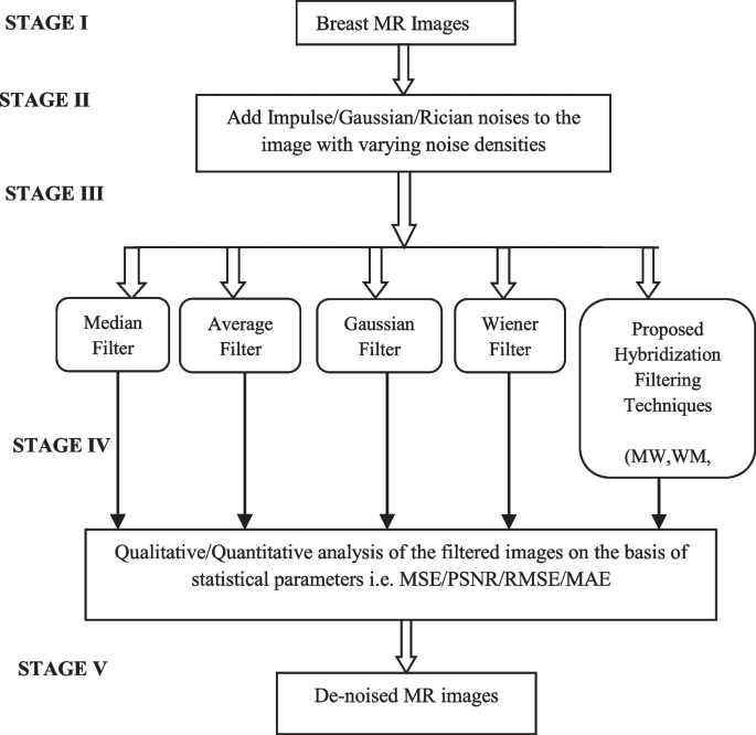
Proposed Methodology
Fig. 7 
Various Breast MR images [17] (a) Breast MR Image 1 (b) Breast MR Image 2 (c) Breast MR Image 3 (d) Breast MR Image 4 (e) Breast MR Image 5
The proposed technique is implemented in MATLAB 2012 (The MathWorks Inc., Natick, MA, USA 2012) environment with 2.19 GHz CPU, 3G RAM with Windows XP system.


4 Results & discussion
In this paper, five different breast MR images are degraded by adding different noises i.e. Impulse, Gaussian& Rician with varying noise densities. Then the pre-processing is done with the proposed hybridization filtering techniques (MW & WM) and the results are compared with the existing filtering techniques discussed in Section 3.
Some other cascading combinations like MWMW, WMWM etc. are also implemented to evaluate the findings in more authentic way and the results clarified the fact that the order of cascading must be in a way that the wiener filter followed by the median filter rather than the reverse one as MWMW provided good results as compared to WMWM, WM and MW.
4.1 Qualitative analysis
As alone quantitative analysis is not sufficient to ensure the efficiency of proposed technique so qualitative analysis of the processed images through proposed technique must be needed which are further verified by experts/radiologists. Figure 2a–e shows the effect of Impulse noise on the original breast MR image as the noise density varies in between 0.05 and 0.5 and the qualitative analysis of Gaussian noise in Fig. 4a–e depicts that the original breast MR image gets more & more degraded as the noise density increases from 0.05 to 0.5.
Similarly Fig. 5a–e gives the qualitative results of original breast MR image affected by Rician noise with gradually increasing noise density ranges in between 1.0 and 2.8. Finally Fig. 8 shows the qualitative analysis of proposed hybridization filters i.e. MW, WM along with other filters i.e. median, average, Gaussian and wiener for comparing their noise removal capabilities with the proposed one. For qualitative analysis Fig. 8a–v shown to experts/radiologists. The experts verified the facts that the resultant output images of proposed techniques are visually good in comparison to output filtered images (as shown in Fig. 8e–p) by Median, Average, Gaussian and Wienerfilter.

Qualitative analysis of different filters including the proposed ones a Original breast MR image 1. b Gaussian noisy breast MR image 1 with noise density 0.3. c Impulse noisy breast MR image 1 with noise density 0.3. d Rician noisy breast MR image 1 with noise density 22. e–g Median filtered breast MR image of (b–d) respectively. h–j Average filtered breast MR image of (b–d) respectively. k–m Gaussian filtered breast MR image of (b–d) respectively. n–p Wiener filtered breast MR image of (b-d) respectively. q–s MW filtered breast MR image of (b–d) respectively. t–v WM filtered breast MR image of (b–d) respectively
Figure 8a represents the original breast MR image 1. Figure 8b represents the breast MR image 1 affected with the Gaussian noise of density 0.3. Figure 8c represents the breast MR image 1 affected with the Impulse noise of density 0.3. Figure 8d represents the breast MR image 1 affected with the Rician noise of density 2.2. Figure 8e–g depicts the average filtered output of breast MR Image 1of Fig. 8b, c & d respectively. Similarly Fig. 8h to j represents the output of median filter in respect of Fig. 8b to d. Figure 8k to m represents the output of Gaussian filter in respect of Fig. 8b to d. Figure 8n to p represents the output of wiener filter with respect to Fig. 8b to d as the input to WF. Figure 8q to s represents the output of MW filter in terms of Fig. 8b to d. Similarly Fig. 8t to v represents the output of WM filter in respect of Fig. 2b to d as the input.
4.2 Quantitative analysis
Tables 1, 2 and 3 shows the effect of noise with various statistical parameters i.e. MSE, PSNR, RMSE and MAE. This qualitative analysis verifies the fact that the noise density is the deciding factor of the type of noise which is more dominant. Tables 4 and 5 illustrate thecomparative analysis of the proposed techniques along with the various filters corresponding to the noisy breastMR images with variable noise density. By this analysis, it is concluded that Median filter is best for removal of the salt and pepper noise and Wiener filter is best in removingGaussian noise among the existing filters but the proposed hybridization filters gives the better results as shown in the graphical representations in Figs. 9, 10, 11, 12, 13, 14, 15 and 16 and their interpretations.

Noise density vs. MSE Graph of various existing and proposed filters for Impulse noise image

Noise density vs. PSNR Graph of various existing and proposed filters for Impulse noise image

Noise density vs. RMSE Graph of various existing and proposed filters for Impulse noise image

Noise density vs. MAE Graph of various existing and proposed filters for Impulse noise image

Noise density vs. MSE Graph of various existing and proposed filters for Gaussian noise image

Noise density vs. PSNR Graph of various existing and proposed filters for Gaussian noise image

Noise density vs. RMSE Graph of various existing and proposed filters for Gaussian noise image

Noise density vs. MAE Graph of various existing and proposed filters for Gaussian noise image
Figure 9 clearly shows that the hybridization technique MWMW gives a higher value of PSNR at the higher noise densities (0.3–0.5) as well as approximately equal values at low noise densities (0.05–0.2) in comparison with other proposed hybridization techniques as well as the existing filters under study.
The proposed hybridization techniques i.e. MW1, WM1, WMWM & MWMW gives comparative values for MSE at low noise density (0.05–0.2) while gives better results at higher noise density (0.3–0.5) than other filters as depicted from Fig. 10. But the MWMW gives best results among all the approaches on the basis of qualitative analysis.
MWMW gives tremendous results in form of RMSE at very high noise density i.e. 0.3–0.5 as compared to other ones while proves to be equivalent at noise densities (0.05–0.3) as clearly shown in Fig. 11.
In the case of MAE, MWMW & MW1 gives equivalent results as median filter throughout the noise density while WMWM & WM1 proves better than other filters except the median filter as clearly indicated by Fig. 12.
Table 5 illustrates the qualitative analysis of proposed techniques as well as the other filters performed only on Gaussian noisy breast MR image 1 with varying noise densities. Also, the graphical representation of the same is shown in Figs. 13 to 16.
Even when the Gaussian noise is considered again the hybridization techniques MWMW & MW1 proves better than all other filters at each noise density. Figure 13 remarks the fact explicitly for proposed techniques.
In Fig. 14, the higher values of PSNR for the proposed techniques again strengthen the concept of hybridization. It clarifies the fact that already existing techniques can be improved effectively by this approach.
Similarly, the hybridization techniques give better results for RMSE also which apparently indicates the improved quality of hybridization with specific sequence as shown in Fig. 15.
In this case for MAE, the MWMW & MW1 is equivalent to median filter while WM1 is better than remaining filter but not good as median filter clearly depicted in Fig. 16.
The comparative analysis of the latest research in this field of MR image enhancement is done in Table 6 for the standard benchmark function for noise removal i.e. SNR and Peak signal to noise ratio (dB) to validate the proposed technique.
These proposed techniques are also tested on the breast MRI data collected from Healthmap, PGIMS, Rohtak. The qualitative analysis done on the MR images corrupted with both the dominant noises i.e., Impulse and Gaussian noises with noise density (20% and 50%).
The visual test report given in Fig. 17 are validated by the experts/radiologists of Govt. as well as private hospitals and proves the fact that the proposed filters are performed well and gives the best results among all the state-of–art methods of noise removal.

a Original Breast MRI of eight patients [1–8 (from left to right)] (b) Average filtered images (c) Gaussian filtered (d) Wiener filtered (e) Median filtered f MW filtered (g) MWM filtered (h) MWMW filtered (i) WM filtered (j) WMW filtered (k) WMWM filtered breast MR Images
5 Conclusion
To ensure the performance of proposed techniques, the qualitative as well as quantitative analyses are done. For qualitative analyses the MR images processed with proposed techniques were shown to experts/radiologists while for quantitative analysis various mathematical parameters i.e. PSNR, MSE etc. were calculated.This paper investigated the fact that the Gaussian noise is the most dominant noise in breast MR images at low noise density (0.05–0.2) while analysis shown in Tables 1 and 2 indicates that at higher noise densities (0.3–0.5), the Impulse as well as Gaussian noise becomes equally dominant. The quantitative analysis given in Tables 4 and 5 concluded that the proposed hybridization approaches i.e. MWMW & MW1give best outcomes for impulse as well as Gaussian noise removal at higher noise densities Similarly,the other proposed techniques i.e. WMWM & WM1 are comparatively better amongotherexisting filtering techniques. The comparison of the proposed noise removal techniques with the standard techniques used for impulse as well as Gaussian noise removal from breast MR images are further validated by the experts which signify its excellent performance and property of preserving the textural features. Through this investigation, it has been concluded that the selection of channels for de-noising the MR pictures rely upon the sort of noise and in addition the noise density. This identifies the fact that the researchers can implement the hybridization combinations of various existing filters in future to enhance the scope of further improvements but the order must be specific. This work can be improved by implementing various distinguished hybridization approaches in a specific order as per the requirement of the particular application.
Data availability
Data sharing not applicable to this article as no datasets were generated or analyzed during the current study.
References
Jaglan P, Dass R, Duhan M (2019) Breast cancer detection techniques: issues and challenges. Journal of The Institution of Engineers (India): Series B Electrical, Electronics & Telecommunication and Computer Engineering, Springer, India, (vol 100 pp 1–8). ISSN 2250 – 2106
Sung H, Ferlay J, Seigal RL et al (2021) Global cancer statistics 2020: GLOBOCAN estimates of incidence and mortality worldwide for 36 cancers in 185 countries. Cancer J Clin 71(3):209–249
Jaglan P, Dass R, Duhan MA (n.d.) Comparative analysis of various image segmentation techniques. Proceedings of 2nd International Conference on Communication, Computing and Networking, Lecture Notes in Networks and Systems, 46. https://doi.org/10.1007/978-981-13-1217-5.36. Springer Nature Singapore Pte Ltd
Al-Faris A, Ngah U, Mat I, Nor A, Shuaib IL (2014) Breast MRI Tumour Segmentation Using Modified Automatic Seeded Region Growing Based on Particle Swarm Optimization Image Clustering. https://doi.org/10.1007/978-3-319-00930-8_5
Jalalian et al (2017) Foundation and methodologies in computer-aided diagnosis systems for breast Cancer detection. EXCLI J 16:113–137
Bhonsle D (2012) Medical image denoising using bilateral filter. Int J Image Graph Signal Process 6:36–43
Bao P, Zhang L (2003) Noise reduction for magnetic resonance images via adaptive multiscale products thresholding. IEEE Trans Med Imaging 22(9):1089–1099
Wong WCK, Chung ACS (2004) A nonlinear and non-iterative noise reduction technique for medical images: concept and methods comparison. Int Congr Ser 1268:171–176
Rajeshwar Dass P, Devi S (2011) Speckle noise reduction techniques. Int J Electron Electr Eng 16(01):47–57
Jafar I, AlNa'mneh R, Darabkh K (2013) Efficient Improvements on the BDND Filtering Algorithm for Removal of High-Density Impulse Noise. IEEE Trans Image Process 22:1223–1232. https://doi.org/10.1109/TIP.2012.2228496
Tian C, Fei L, Zheng W, Xua Y, Zuo W, Lin C-W (2020) Deep learning on image denoising: an overview. Neural Netw 131:251–275
Patil J, Jadhav S (2013) A comparative study of image denoising techniques. Int J Innovative Res Sci Eng Technol 2(3):2319–8753
Mahmood MT et al (2016) Rician noise reduction in magnetic resonance images using adaptive non-local mean and guided image filtering. Opt Rev 23(3):460–469
Nowak RD (1999) Wavelet-based rician noise removal for magnetic resonance imaging. IEEE Trans Image Process 8:10
Saini S, Kumar V, Dhiman S (2012) Quality Improvement on MRI Corrupted with Rician Noise Using Wave Atom Transform. Int J Comput Appl 37(8):28–32. https://doi.org/10.5120/4630-6665
Isa IS et al (2015) Evaluating denoising performances of fundamental filters for T2 weighted MRI images. In: Proceedings of the19th International Conference on Knowledge Based and Intelligent Information and Engineering Systems, Procedia Computer Science, (vol 60, 1877 – 0509, pp 760–768)
Mehta R, Aggarwal NK (2014) Comparative analysis of median filter and adaptive filter for impulse noise – a review. In: The Proceedings of National Conference on Recent advances in Wireless Communication and Artificial Intelligence, pp 30–34
Swapna M, Hegde N (2023) Noise removal filtering methods for mammogram breast images. https://doi.org/10.1007/978-981-19-8086-2_97
Sivasundari MKS, Kumar RS (2014) Performance analysis of image filtering algorithms for MRI images. Int J Res Eng Technol 3(5):438–440
Kwan BYM, Kwan HK (2011) Impulse noise reduction in Brain magnetic resonance imaging using fuzzy filters. Int J Med Health Biomed Bioeng Pharm Eng 5:12
Ambule V, Ghute M, Kamble K, Katre S (2013) Adaptive median filter for image enhancement. Int J Eng Sci Innovative Technol 2(1):318–323
Gonzalez RC, Richard E (2009) Woods. Digital image processing. 3rd edition, Pearson Education International
Rajeshwar Dass S, Devi P (2012) Effect of Wiener- Helstrom Filtering cascaded with bacterial foraging optimization to Despeckle the Ultrasound Image. Int J Comput Sci Issues 9(4):2
Dass R (2018) Speckle noise reduction of Ultrasound images using BFO cascaded with Wiener Filter and Discrete Wavelet transform in Homomorphic Region ICCIDS. Procedia Comput Sci 132:1543–1551
Saleh MD, Eswaran C (2012) An automated blood vessel extraction algorithm in fundus images. In: The Proceedings of IEEE International Conference on Bioinformatics and Biomedicine, pp1–5
Rani SHS, Godwin PMS (2015) Comparative analysis of various wavelets for denoising Color images. ARPN J Eng Appl Sci 10(9):3862–3867
Jinrong H (2012) Improved DCT-based nonlocal means filter for MR images denoising. Comput Math Methods Med 2012:232685
Rajeshwar Dass S (2014) Performance analysis of acoustic echo cancellation techniques. IJERA 4(7):172–180
Swapna M, Hegde N (2023) Noise Removal Filtering Methods for Mammogram Breast Images. https://doi.org/10.1007/978-981-19-8086-2_97
Sánchez MG et al (2012) Medical image restoration with different types of noise. In: The Proceedings of the 34th Annual International Conference of the IEEE Engineering in Medicine and Biology Society San Diego, California USA, September, pp 4382-5
Nirmal A, Raval P, Patel S (2020) Analysis of image denoising techniques with CNN and residual networks in deep learning. J Interdiscip Cycle Res 12:222–246
More S, Singla J, Song O-Y, Tariq U, Malebary S (2021) Denoising medical images using deep learning in IoT environment. Comput Mater Contin 69:3127–3143 ([CrossRef])
Trung NT, Trinh D-H, Trung NL, Luong M (2022) Low dose CT image denoising using deep convolutional neural networks with extended receptive fields. Signal Image Video Process 16:1963–1971
Thayammal S, Sankaramalliga G, Priyadarsini S, Ramalakshmi K (2021) Performance analysis of image denoising using deep convolutional neural network. IOP Conf Ser Mater Sci Eng 1070:012085 ([CrossRef])
Zheng D, Tan SH, Zhang X, Shi Z, Ma K, Bao C (2020) An unsupervised deep learning approach for real-world image denoising. In: Proceedings of the International Conference on Learning Representations, Addis Ababa, Ethiopia, 26–30 April, pp 1–12
Izadi S, Sutton D, Hamarneh G (2022) Image denoising in the deep learning Era. Springer Nature, Dordrecht, The Netherlands, pp 1–59
Vimala BB, Srinivasan S, Mathivanan SK, Muthukumaran V, Babu JC, Herencsar N, Vilcekova L (2023) Image noise removal in ultrasound breast images based on hybrid deep learning technique. Sensors 23:1167
Author information
Authors and Affiliations
Corresponding author
Ethics declarations
Conflict of interest
The authors declare that they have no conflict of interest.
Additional information
Publisher’s Note
Springer Nature remains neutral with regard to jurisdictional claims in published maps and institutional affiliations.
Rights and permissions
Springer Nature or its licensor (e.g. a society or other partner) holds exclusive rights to this article under a publishing agreement with the author(s) or other rightsholder(s); author self-archiving of the accepted manuscript version of this article is solely governed by the terms of such publishing agreement and applicable law.
About this article

Cite this article
Jaglan, P., Dass, R., Duhan, M. et al. Effective hybridization approach for noise removal in magnetic resonance imaging. Multimed Tools Appl (2024). https://doi.org/10.1007/s11042-024-18663-5
Received:
Revised:
Accepted:
Published:
DOI: https://doi.org/10.1007/s11042-024-18663-5