
Abstract
Wireless data transmission on the Internet of Things (IoT) needs data-aware communication protocols. Clustering is one of the effective network management approaches that enhance the lifetime of IoT. The primary challenge in the data transmission across IoT is designing an energy-efficient clustering mechanism. Existing protocols struggle with the non-optimal selection of CHs and frequent re-clustering on IoT, which leads to significant energy consumption. If the cluster head (CH) lifetime of the devices (nodes) is known prior, then re-clustering can be avoided to a reasonable extent. Therefore, in this paper, we estimate the lifetime of devices as CHs by solving a linear optimization problem to extend the first node death as much as possible and also, stalls the frequent re-clustering process to minimize the energy consumption. We also apply the uniform distribution of CHs to ensure balanced energy consumption on IoT devices. The proposed clustering technique named ECFEL (Efficient Clustering using Fuzzy logic based on Estimated Lifetime) for IoT outperforms the existing protocols, namely Low Energy Adaptive Clustering Hierarchy (LEACH), MODified LEACH (MOD-LEACH), Dynamic k-LEACH (DkLEACH), Novel-PSO-LEACH, FM-SCHEL, and M-IWOCA techniques in terms of first node death (FND), half node death (HND), last node death (LND). Our simulation results showcase that ECFEL is having a better lifetime in terms of FND, HND, and LND, respectively. Furthermore, the experiments also confirm that ECFEL consumes less energy while maintaining a packet delivery ratio for a more extended period.
1 Introduction
The Internet of Things (IoT) has evolved as a prominent research field in the past decade. IoT consists of identical smart and wireless objects and individuals who can transmit data over the network independently. Various studies forecast that the IoT marketplace will rise from 158B in 2016 to 550B dollars by 2021. They have left an imprint in a massive variety of applications relating to smart homes, smart industry, logistics and transportation, smart cities, smart retails, and connected cars, etc. [2, 12, 17, 26, 30, 33]. Wireless sensor networks (WSNs) have a very significant role in the development of an aspect of the IoT. They function as a virtual membrane where the information about the physical world can be read and interpreted by a computational framework. A WSN is a composition of numerous intelligent, low-power sensor devices and a high-powered sink [18, 39]. Wireless devices periodically transmit data to the base station. These sensors used in sensor networks are having many constraints, such as limited energy, memory, processing ability [5, 40]. According to energy models, transmission and reception costs are significant drains on the batteries of the sensors [9]. Therefore, achieving an energy-efficient data transmission from the source to the target devices is one of the significant difficulties confronting the IoT. Also, redundancy in the sensed data occurs usually when multiple devices may sense the same area [1, 25]. The communication of this redundant data consumes much energy.
The usage of clustering can minimize this energy consumption. Clustering operations are the most promising approaches to resolve these issues [11]. Clustering reduces the number of transmissions, exploits the resemblance in the sensed values collected from nearby sensor devices for aggregation, and hence, reduces the energy consumption compared to a non-clustered environment. In clustering, the network of sensor devices is divided into clusters. These devices (i.e., cluster member (CM)), instead of sending the data directly to the BS, transmit their data via specially selected nodes termed as cluster heads (CHs) to the BS as illustrated in Fig. 1.

Clustering Architecture in WSNs
Existing clustering techniques have several drawbacks, namely: a) Residual energy is not accounted in the election of CHs in LEACH. It may lead to a possibility that inefficient CHs get selected, which results in early first node death. b) CHs rotation is done after every round which increases further energy consumption and a delay. c) CHs may get selected very close to each other, thereby losing the effectiveness of the clustering approach. It happens because of non-uniform selection of CHs. d) The effect of these shortcomings becomes evident in large-scale networks where these techniques could not perform up to the mark. Ensuring uniform CHs selection and estimating when to perform the next re-clustering is an arduous task. In this paper, we have tried to improve these processes by confirming the selection of CHs uniformly throughout the monitoring area and stalling the re-clustering on IoT under safe limits. In other words, re-clustering on IoT is deferred utmost until one of the selected CHs completes its lifetime as CH, which is estimated through a linear optimization problem. CHs lifetime values along with other vital parameters are utilized for fuzzy logic-based clustering on IoT. They employ fuzzy logic to handle the uncertainties and complexity of WSNs. We will discuss such techniques in the next section.
1.1 Contributions
Our contributions in this paper are in the following order:
-
a)
We estimate the lifetime of each device as CH and CM using linear optimization. The estimated lifetime of the device as CH helps in the optimal selection of CHs and reduces the frequency of re-clustering process for the efficient working of IoT.
-
b)
We propose to use fuzzy logic to establish a relationship between the value of three parameters viz normalized value of residual energy, node centrality, estimated device’s lifetime as a CH, and the chances that a node becomes a CH.
-
c)
We have used the estimated CH lifetime of selected CHs to reduce the overheads of the re-clustering process on IoT.
-
d)
We have suggested a different strategy for uniform selection of the CHs.
-
e)
All the contributions are utilized to propose a routing protocol, ECFEL. To showcase the benefits of the variable estimated with linear optimization, we have considered a different technique named ECF. We then compare the proposed protocol with prominent protocols LEACH [10], MOD-LEACH [20], Dk-LEACH [6], Novel-PSO-LEACH [36], FM-SCHEL [38], and M-IWOCA [31]. Comparative analysis confirms proposed ECFEL is doing better than these techniques, even for large-scale IoT.
The rest paper is structured as follows: In Section 2, we discuss the state of the art fuzzy based clustering techniques on IoT. In Section 3, we discuss the IoT model and energy model. In Sections 4.1 to 4.3, we discuss the proposed technique in detail. In Sections 5 and 6, simulation results and conclusion are discussed respectively.
2 Literature review
The fundamental limitation in the design of WSNs assisted IoT is the frequent battery drain-off due to numerous reasons [41]. In literature, different clustering-based protocols have been suggested to address the same [22]. The primary goal is to organize IoT devices through specific clusters, thereby ensuring power consumption and hierarchical management.
2.1 Clustering protocols on IoT and WSNs
Clustering serves as a boon to enhance the network lifetime. Authors in MOD-LEACH [20] have proposed a clustered approach to elongate the network lifetime. Initially, CHs are selected in the same way as in LEACH algorithm. Although, in the MOD-LEACH algorithm, re-clustering is done only when a CH consumes energy more than a certain threshold which is decided arbitrarily. This may not be a good criterion to demote a device from being CH. Also, CHs may get selected very close to each other, thereby losing the effectiveness of the clustering approach. In DK-LEACH [6], authors have proposed a comprehensive approach of popular LEACH algorithm to minimize the energy consumption of the unevenly distributed network. In DK-LEACH, only those nodes with more energy than the average energy of the network are accounted as the candidates for CH selection. A function having the proportion of the distance between CHs and non-CHs, and the surplus energy is found out. The minimum value of the function shows selected CH has a lesser distance to the nodes and higher remaining energy. Then node density is used to adjust the proportion. However, CHs rotation is done after every round, and uniform selection of CHs is not ensured, which leads to more and non-uniform energy consumption in the network.
To mitigate the issues of energy consumption in WSNs, a particle swarm optimization (PSO) based clustering protocol is suggested [36]. CHs are selected using PSO based approach. The fitness value of the particles is evaluated based on the remaining energy of that node and the distance of the node to the base station. But, re-clustering is done after every round, which is purely an overhead process and reduces network lifetime. A two-level unequal clustering protocol on IoT is introduced by sharing the incoming traffic to enhance the system performance [8]. The goal is to minimize the number of CHs. To achieve the same, IoT devices are grouped optimally in unequal-sized clusters. Authors have selected the primary CH to the device having the highest node degree in the monitoring area. The secondary CHs selection process is done based on remaining energy and node degree. This process stops when all devices are attached to at least one cluster. Nevertheless, having many layers in hierarchical clustering can increase the number of hops, which further extends the delay. LEACH protocol is extended by proposing a low-powered adaptive layered mechanism based on clustering [42]. The authors have given the focus on traffic load analysis and network reliability while designing their mechanism. However, the authors have not paid attention to the uniform selection of CHs, which increases energy consumption.
Authors [4] have presented a CHs selection protocol on IoT based on a multi-objective fractional gravitational search algorithm. Fitness function objectives include delay, remaining energy, the distance between devices, link lifetime. However, they have not tried to decrease the re-clustering process, which incurs energy consumption. Authors [34] have achieved better network throughput by suggesting a clustering protocol based on load-balancing and delay minimization. Uniform and non-uniform incoming traffic are handled for IoT applications by utilizing a multi-objective cost function-based simulated annealing. Cost function includes distance between CHs and IoT devices, the distance between CHs and BS, and incoming traffic. Moreover, the solution provided by the simulated annealing does not ensure that solution will converge to optimal value and can fall into local optimum in most cases. Authors [15] have minimized the communication cost for large-scale wireless mesh networks. They have proposed a delay-aware clustering protocol on IoT that groups the IoT devices in four different clusters to achieve the same. Cluster is formed on behalf of one-hop neighbors i.e. null, CHs, cluster members, and cluster relay devices. Although, uniform clustering is not adequately ensured. To lessen the total number of wireless links on IoT, authors [35] have presented a multi-hop heuristic-based clustering protocol. The primary objectives of this protocol are to minimize the total CHs, and distance between IoT devices and CHs. This protocol provides the optimal clusters with minimum connections on both small and large IoT models. However, the authors have not given the focus on minimizing the re-clustering process.
2.2 Fuzzy logic-based clustering protocols on IoT and WSNs
Although clustering is one of the energy-efficient techniques, CHs selection is computationally complex and expensive [27]. The benefits provided by clustering outway the computational complexity and the cost incurred. Fuzzy logic handles the complexity, thereby making things more comprehend-able [7, 16, 23]. Therefore, many researchers proposed to use the fuzzy logic-based clustering [32]. Even in the absence of complete information, real-time decision-making can be done using fuzzy logic controllers (FLCs). Considering the above benefits of fuzzy logic, several protocols aiming towards ameliorating lifetime have used this technique. To minimize the total energy consumed in the network, a two-level hierarchical protocol based on fuzzy logic is proposed [38]. CHs and super CHs are selected using fuzzy logic which utilizes node degree, node centrality, and battery power to calculate the chance of election value. However, the authors have not focused on minimizing the re-clustering process and making uniform energy consumption. Then, to make the network energy-efficient and to elongate the network lifetime, an evolutionary approach and fuzzy logic-based solution is suggested [31]. Authors have used fuzzy logic to estimate the fitness value for which the fuzzy descriptors are taken as node degree, centrality, residual energy, and distance to BS. Then, invasive weed optimization (IWO) is utilized to select the candidate CHs for a round, and thereafter final head nodes are selected with the help of genetic algorithm and IWO. On the contrary, this approach also leads to more energy consumption because of frequent re-clustering in every round, and the evolutionary approach does not ensure the optimal solution.
Authors [28] have utilized fuzzy logic to present a quality of service based energy-efficient clustering protocol for WSNs assisted IoT. CHs and cluster devices are selected using fuzzy logic based on multiple parameters involving link quality of devices, the distance between IoT devices, and remaining energy. This multi-criteria-based decision-making helps in minimizing the energy consumption of IoT devices, network lifetime, and transmission delay. Authors [37] presented an energy-efficient data communication clustering based protocol on IoT. In this three-layer protocol, the sink decides the upper CHs using fuzzy c-means algorithm that involves the parameters residual energy and location of IoT devices. While IoT devices select the lower CHs in a distributive way that limits the exchange of control packets. An unequal clustering-based protocol was suggested in which CHs selection was made based on decisions taken by FLCs [3]. The input parameters considered were distance to BS and residual energy. However, the authors had not considered the local distance from the surrounding devices. Another multi-objective clustering technique that utilized fuzzy logic was proposed to address the hotspot and energy hole problem [29]. In this paper, the authors had considered the distance to sink, node centrality, and residual energy to determine the competition radius. The local distance was considered, as well. Yet, they did not emphasize uniform energy consumption, so the selected CHs might be very close or far to each other. An improved version of [3] was presented by [19]. Authors in [19] had accounted for one more parameter compared to [3] which was node degree, for the election of CHs. Fuzzy logic with two variables i.e., distance and node degree of CH, was considered during cluster formation. It also required re-clustering after every round. Other authors had used a fuzzy-based clustering approach [14]. In this work, the authors had accounted for expected residual energy. Chances for CHs selection were dependent on residual energy as well as expected residual energy. Nevertheless, it had not focused on the uniform selection of CHs.
2.3 Analysis of clustering protocols
The protocols discussed above upgrade the efficiency of IoT to some extent. However, they had their issues like probabilistic clustering, frequent re-clustering, etc. Heuristic methods provide an approximate solution to the clustering problem. They focus on reducing the number of clusters that unbalances the traffic load and minimizes the IoT lifetime. While the meta-heuristic methods emphasize remaining energy and distance but ignore the node centrality. Both heuristic and meta-heuristic-based protocols have not emphasized stalling the re-clustering process which is purely an overhead and incurs a lot of energy consumption. To overcome those problems, many authors have proposed many different protocols. However, they have their issues like probabilistic clustering, frequent re-clustering, etc. To avoid the problem of re-clustering, the authors of MOD-LEACH have attempted. But, the downside of the work is, as the energy consumption of any CH goes below a particular threshold, that CH is replaced with new CHs selected by the LEACH technique. They have used different power levels for intra and inter CHs communication which is not showing any significant difference in the experimental results. To avoid the problems like non-optimal and non-uniform CHs selection, frequent re-clustering, we have proposed this technique, which reaps the benefits of fuzzy logic and linear optimization. A summary of objectives, critical parameters considered, methodology used, and outcomes of the reviewed clustering protocols examined is shown in Table 1.
3 System model
3.1 IoT model
In this paper, we model the IoT as follows: dimension of the monitoring area is considered as M × M. A set of n sensor devices is randomly deployed over the entire area with uniform distribution. \(\hat {S}\) is representing the set of devices. A unique ID is assigned to all the sensor devices. Sensor devices are stationary and location-aware. Euclidean distance between all the sensor devices (dij) is determined by using the received signal strength. When required, the sensor devices can change their transmitting power level. To solve the linear optimization, MATLAB libraries and functions are used by the sink.
3.2 Energy model
To estimate the energy consumption, we have considered the radio model [10]. The energy consumed in transmitting a packet of κ-bits to the BS is given as:
where \(\mathbb {E}_{elec}\) represents the amount of energy required to activate the electronic circuits. 𝜖fs (free space) and 𝜖mp (multi-path) are the energy required by amplifier. Here dij is euclidean distance between sensor devices si and sj. While the energy consumed by sensor device si in receiving a packet from its neighbor sk is given by:
4 Proposed technique
In this section, we discuss the overall functioning of our proposed fuzzy-based clustering technique for IoT (ECFEL). Its goal is to increase the overall lifetime of IoT while reducing the energy requirement of the protocol. Our technique works in four phases: network initialization, parameters evaluation, CHs selection and data transmission on IoT, and ECF technique. In network initialization phase, required information is collected ((explained in depth in Section 4.1)) to calculate the parameters such node centrality, residual energy, and each device’s lifetime as a CH (discussed in Section 4.2). These parameters are embedded into fuzzy logic to finally select the uniformly distributed CHs to prolong the IoT lifetime (detailed explanation in Section 4.3). Also, time of re-clustering is calculated using estimated CH lifetime. Once estimated lifetime of each CH is exhausted, the residual energy is utilized by delegating decisions of making CH to ECF as last attempts to keep the network alive as long as possible. In the next sections, we will discuss in detail all the above-discussed phases which are summarized in Fig. 2.

4.1 Network initialization
To discover network topology, every device broadcasts a RQST message into the monitoring area to know about one hop neighboring devices. Each IoT device (si) prepares a neighbor list \(\mathcal {N}_{i}\) of all the one hop away sensor devices, from which RQST messages are received. This information along with residual energy REi, initial energy IEi, network topology of the IoT device is then sent towards the BS. Once the information about the network structure and energy is reached at the sink, it calculates number of neighboring devices w.r.t. each device i.e. node degree, distance between the pair of devices, energy consumption of each device as a CH and as CM are calculated by sink as discussed in Section 4.
-
(i)
Count of devices that are in the communication range of each IoT device or node degree is calculated as:
$$ ND_{i} = |\mathcal{N}_{i}| $$(3) -
(ii)
Sum of the squared distance (χi) of each IoT device (si) from the rest of the devices is calculated as:
$$ \chi_{i} = \sum\limits_{j \in \mathcal{N}_{i}}d_{ij}^{2} $$(4) -
(iii)
Energy consumption of a IoT device as a CH and CM are found out as described below. Let
-
ERki is the energy consumed during the receiving of one packet (having κ − bits) from device sk (where device sk can be CM or CH) to device si (which is either CH for a CM or Next Hop (NH = CH or BS) for a CH). In other words, communication will always be among: (CM, CH) or {(CH, CH) | (CH, BS)}. The ordered pair (a,b) means that a device transmits the data to b. This consumption is calculated as stated in the energy model in Section 3.2.
-
ETij is the energy consumed during the transmission of one packet from device si to device sj, where device si can be CM or CH and device sj can be CH or relay CH or BS for other CHs.
-
When a IoT device si transmitting the data to IoT device sj, energy consumption rate in sending one packet is calculated as (energy consumption w.r.t. a single packet is given by energy model, defined in Section 3.2)
$$ ET_{ij} = \begin{cases} \mathbb{E}_{elec} \times \kappa + \epsilon_{fs} \times \kappa \times d_{ij}^{2}, & d_{ij} < d_{TH}\\ \mathbb{E}_{elec} \times \kappa + \epsilon_{mp} \times \kappa \times d_{ij}^{4}, & d_{ij} \geq d_{TH} \end{cases} $$(5)Here dij is euclidean distance between sensor devices si and sj.
-
Energy consumption rate in receiving one packet (ERki) by IoT device si from its neighbor sk is a constant value. It is given by energy model as stated in Section 3.2.
-
EGi is the energy consumed during the sensing in one round. This value is same for every IoT device.
-
\(\zeta _{ij}^{CM}\) depicts how much energy a cluster member si consume in a single round where j is its CH.
$$ \zeta_{ij}^{CM} = ET_{ij} + EG_{i} $$(6) -
\(\zeta _{ij}^{CH}\) depicts how much energy a cluster head si consume in a single round where j is si’s NH.
$$ \begin{array}{@{}rcl@{}} \zeta_{ij}^{CH} = EG_{i} + ER_{ki} \times Pkts^{recvd}_{i} + ET_{ij} \end{array} $$(7)where \(Pkts^{recvd}_{i}\) represents the number of packets that have been received by a IoT device si from its neighbors. \(\zeta _{ij}^{CH}\) is dependent on the number of member devices in the cluster and ETij is dependent on the distance between ith CH and its NH.
-
Total energy consumption is found using:
$$ \begin{array}{@{}rcl@{}} \zeta_{total}^{i} = EL^{CH}_{i} \times \zeta_{ij}^{CH} + EL^{CM}_{i} \times \zeta_{ij}^{CM} \end{array} $$(8)
-
Here \(EL^{CH}_{i}\) and \(EL^{CM}_{i}\) depicts the estimated lifetime of a IoT device si as a CH and CM respectively.
- Note: :
-
There is no initial knowledge about the clusters formation in the network. Therefore, to evaluate \(EL^{CH}_{i}\) and \(EL^{CM}_{i}\) before the formation of cluster, some assumptions need to be taken specially the estimates of distance between the sender and receiver to estimate the energy consumption of transmitter and number of cluster members to estimate the energy consumption of receiver. So, we have estimated: (i) number of packets a CH can receive in (7), (ii) distance between CM and CH while finding ETij in (6) (dij = dCM,CH, when a device si is treated as CM), and (iii) distance between CH and NH while finding ETij in (7) (dij = dCH,NH, when a device si is treated as CH).
To estimate above mentioned parameters by examining the behavior of the stated network and energy model, we have analyzed three scenarios: worst, average, and realistic case which are discussed below.
-
(a)
Worst Scenario is the scenario that causes maximum energy consumption.
-
(1)
When a IoT device si is treated as CM, its energy consumption during transmission is found by assuming that its CH is communication radius (CR) away (that is furthest away but in communicable range). The maximum distance between any CM and its respective CH is given by:
$$ Max\_d_{CM,CH} = CR $$ -
(2)
Maximum number of packets that a CH si can receive, is equal to total devices which fall in its communication range i.e.
$$ Max\_Pkts^{recvd}_{i} = ND_{i} $$ -
(3)
Similarly, when a IoT device si is treated as CH, the data is assumed to be sent directly to the sink. Therefore, the maximum distance of a CH w.r.t. its NH is given by:
$$ Max\_d_{CH,NH} = d_{i,BS} $$Here, di,BS represents the distance of device si from the sink.
-
(1)
-
(b)
Average Scenario is the scenario that estimates expected energy consumption over a large number of experiments.
-
(1)
When a IoT device si is treated as CM, its energy consumption during transmission is found by assuming that its CH is at an average distance. The average distance between any CM and its respective CH is given by:
$$ Avg\_d_{CM,CH} = \frac{\sqrt{{\sum}_{i=1}^{ND_{i}} d_{ij}^{2}}}{ND_{i}}, where\ j \in \mathcal{N}_{i} $$ -
(2)
On an average, number of packets that a CH (si) can receive, is calculated as:
$$ Avg\_Pkts^{recvd}_{i} = \frac{n-\hat{p}}{\hat{p}} $$where n and \(\hat {p}\) are number of total devices and selected CHs respectively.
-
(3)
When a IoT device si is treated as CH, it will transmit its data towards the sink. The average distance of a CH w.r.t. its nearest possible next CH is given by (using Pythagorean theorem):
$$ Avg\_d_{CH,NH} = \Biggl\lceil{\frac{\sqrt{5}M}{g}}\Biggr\rceil $$where M is the monitoring area dimension and \(g = \sqrt {\hat {p}}\)
-
(1)
-
(c)
Realistic Scenario We have discussed the extreme case and an average case so far. Things may not exactly match these situations in reality. Therefore, to approximate the model and analyze the situation better, the values of these parameters are tuned between these two scenarios for better estimation of lifetime of CH corresponding to all the devices.
-
(1)
$$ d_{CM,CH} = \varphi \times Max\_d_{CM,CH} + (1 -\varphi) \times Avg\_d_{CM,CH} $$
-
(2)
$$ Pkts^{recvd}_{i} = \xi \times Max\_Pkts^{recvd}_{i} + (1-\xi) \times Avg\_Pkts^{recvd}_{i} $$
-
(3)
$$ d_{CH,NH} = {\varsigma} \times Max\_d_{CH,NH} + (1-{\varsigma}) \times Avg\_d_{CH,NH} $$
where φ, ξ and ς lie in the range [0,1]. These are the parameters to be tuned experimentally.
-
(1)
4.2 Parameters evaluation
In ECFEL, we have taken three input variables, namely residual energy (RE), node centrality (NC), an estimated lifetime of a IoT device si as a CH (\(EL^{CH}_{i}\)) (in rounds). By the difference in the results of ECF and ECFEL, we can analyze that the third input variable and delayed re-clustering play a significant role. This helps to improve lifetime by mitigating energy consumption. The consumption occurs during the re-election and re-clustering process. This variable is estimated by solving a linear optimization problem. Parameters are calculated as follows:
-
(i)
Residual energy (RE): The devices having higher remaining energy are more favorable for the election of CHs. So, residual energy is kept into account. To utilize the value of RE in FLC, residual energy is adjusted in the range [0,1]. The goal behind normalization is to take different scales value on to a single standard scale. It results in the same effect of all the variables. Normalized value of RE of a device si can be stated as:
$$ Norm\_RE_{i} = \frac{RE_{i}}{IE_{i}} $$(9)Here, REi represents current energy.
-
(ii)
Node centrality (NC): The device’s energy consumption depends on how many devices it is surrounded and how far it is from them. The higher the number of surrounding neighbors and the lower the local distance from them, the lower the energy consumption. Hence, node centrality is kept into account. Node centrality of a device is defined as the square root of the ratio of summation of the squared distances from the neighbors (defined in (4)) to the node degree i.e.
$$ NC_{i} = \sqrt{\frac{\chi_{i}}{ND_{i}}} $$To utilize the value of NC in FLC, NC is also normalized to adjust its value in between 0 and 1. The normalized value of NC of a device si is can be written as follows:
$$ Norm\_NC^{i} = NC_{i}/CR $$(10)Here, CR is the communication range.
-
(iii)
Estimated lifetime as a CH (\(EL^{CH}_{i}\)): In this proposal, we have considered a novel parameter, which has not yet accounted for selection of CHs. This input variable is calculated by using (8) in the linear problem formulation. The solution of the same gives us the lifespan of the IoT devices as CHs and CMs, which is further used in the CHs selection and re-clustering process. The lifespan of the device that will die first is maximized to increase the network lifetime. We also expect that in the end, the total energy of each device should be consumed. Accordingly, the objective function is defined as:
$$ \max_{EL^{CH}_{i} EL^{CM}_{i}} (\min_{i} (EL^{CH}_{i} + EL^{CM}_{i})) $$(11)subject to
$$ \begin{array}{@{}rcl@{}} \zeta_{total}^{i} = IE_{i} \end{array} $$(12)$$ \begin{array}{@{}rcl@{}} EL^{CH}_{i} = \frac{EL^{CM}_{i}}{T-1}, where\ T = n/\hat{p} \end{array} $$(13)$$ \begin{array}{@{}rcl@{}} EL^{CH}_{i} \geq 0 \end{array} $$(14)$$ \begin{array}{@{}rcl@{}} EL^{CM}_{i} \geq 0 \end{array} $$(15)The objective function (11) is showing that the IoT device which is having a minimum lifetime should be maximized to stall the first node death. The constraint in (12) is representing that at the end total energy of all the devices get consumed. Equations (14) and (15) constraints are showing the life of a IoT device as a CH and as CM should be greater than or equal to 0. If we assume that all the devices will be alive equally long i.e., T slots where a slot is the minimum number of rounds for which any IoT device may work as CH. Also, each IoT device can work as a CH in one slot only. Further, assuming that all the slots are having an equal number of rounds. Then, for any IoT device \(EL^{CH}_{i}\) is proportional to 1 slot duration while \(EL^{CM}_{i}\) is proportional to T − 1 slot duration. But, we also know that ideally there will be \(\hat {p}\) CHs at point of time before FND. Therefore, number of slots must be \(n/\hat {p}\) which is represented by (13). Further, (11) can be more simplified into (16) by adding one more constraint (motivated from [24]). Hence, the above formulation can equivalently be written as:
$$ \max z $$(16)subject to
$$ \begin{array}{*{20}l} 0 \leq z \leq EL^{CH}_{i} + EL^{CM}_{i}\\ \zeta_{total}^{i} = IE_{i}\\ EL^{CH}_{i} = \frac{EL^{CM}_{i}}{T-1}, where\ T = n/\hat{p}\\ EL^{CH}_{i} \geq 0\\ EL^{CM}_{i} \geq 0 \end{array} $$LPP returns \(EL^{CH}_{i}\) which indicates for how many rounds, an IoT device should be able to act as CH in IoT. As discussed earlier, once the value of \(EL^{CH}_{i}\) for each IoT device is obtained, normalized value of input variables corresponding to each device i.e., REi, NCi, and \(EL^{CH}_{i}\) are passed to the FLC. Corresponding to the input variables, the output variable is CE is evaluated with inference rules given in Table 2. The higher value of CE of a sensor IoT device favors the device for the final election of CH. The whole procedure is segregated into two phases i.e., uniformly distributed CHs selection phase and cluster formation phase. When the clusters are formed, data transmission starts. In the next section, we will explore how to select the CHs by using CE values which influences the IoT lifetime. We will also see how to pick the CHs uniformly and how to minimize the overheads due to re-clustering.
4.3 Cluster heads selection and re-clustering process on IoT
The chance of election value (CE) corresponding to each IoT device changes dynamically in the proposed technique. Because while finding the CE value, it uses normalized values of RE, NC, and \(EL^{CH}_{i}\). No fuzzy-based clustering techniques have considered the lifespan of a IoT device as CH (\(EL^{CH}_{i}\)) as a parameter to FLC. This novel parameter is considered in our proposed technique. All the input variables should adopt fuzzy linguistic values to pass them to FLC. In Tables 2 and 3, sparse, normal, and dense are fuzzy linguistic values correspond to the input variable Node Centrality. While Remaining_Energy has low, medium, and high as the fuzzy linguistic values. Small, medium, and large are the fuzzy linguistic values for the lifespan of a IoT device as CH \(EL^{CH}_{i}\). All are having the triangular membership function with peak values at 0, 0.5, and 1 corresponds to three linguistic values of all input variables. The output variable is chance of election (CE) value, which has low, medium, and high as the fuzzy linguistic values. For this as well, triangular membership function with peak values at 0, 0.5, and 1 is considered to low, medium, and high, respectively. While deciding the fuzzy rules as given in Table 2, an argument has been considered that when energy and the number of rounds a IoT device can serve as CH are low, it is a wise decision to reduce the chances of those devices. Crisp values are fuzzified into linguistic variables by the fuzzy inference engine. Membership functions that have been defined by the user are used. We have used the Mamdani method, which processes fuzzified input variables and develops fuzzy rules. Inference rules used in ECFEL are listed in the Table 2.
Each time when re-clustering happens, \(\hat {p}\) cluster heads are selected from all devices while ensuring the uniform distribution of selected CHs over the entire monitoring area. CHs are selected based on higher CE values. First CH selection is done using the largest CE value. Successive CHs will only be selected if they are a fixed distance threshold (i.e. dCTH which is 1.5 times of communication range) apart from each of the previously elected CHs and has high CE value among them. This process will continue until a desired number of CHs do not get selected. In this manner, uniform selection of CHs on IoT is ensured as depicted in Fig. 3.
- Cluster Formation and Data Transmission on IoT :
-
As noted above, all CHs are selected by using the CE values, which are determined by the sink. CHs broadcast a CH_Advt message into the monitoring area. When a IoT device receives the information about this, it sends a CH_Join_Rqst message to the nearest CH. When the corresponding CH gets this message, an acknowledgment is sent in return. In this manner, all the devices select their CHs in IoT, and hence clusters are formed. Once the CHs selection phase is over, sensing and data transmission phase on IoT gets started. Communication is carried out in a multi-hop fashion to minimize battery dissipation.
- Stalling Re-Clustering Process on IoT :
-
As we discussed in Section 1, re-clustering is purely an overhead and is done to balance the energy consumption among all the devices. The re-clustering process helps in avoiding the exploitation of a single IoT device for the benefit of the group. But during re-clustering, a lot of energy is consumed. So, in the proposed technique, we have contributed in this direction as well to mitigate the total energy consumption that occurred in re-clustering. The process of frequent re-clustering is avoided by using the parameter \(EL^{CH}_{i}\). The idea of slot duration is introduced to reduce the overheads which occur during re-clustering. Because when slot duration is used, the re-clustering process happens only when the slot duration gets over. In ECFEL, at any instant, once the CHs are selected, they act as CHs for a fixed slot duration. The value of the slot duration is given by minimum among the \(EL^{CH}_{i}\) values corresponding to the elected CHs at any instant. Once the slot duration gets over, the re-clustering is done again. The same process will continue until all the devices can’t complete their slot duration as a CH. Once all the devices have completed their \(EL^{CH}_{i}\), re-clustering happens in each round as in LEACH till all the devices become dead. But now in place of three variables as in ECFEL, we pass only two variables i.e., NC and RE in fuzzy logic. We name it as the ECF method in Figs. 2 and 4. Inference rules used in ECF method are discussed in the Table 3.

Cluster heads selection procedure

Clustering using ECF(NCi,REi) method, takes as input, two variables NC and RE, which are passed to fuzzy logic. CHs selection is done using the method given in Fig. 3. Circled B is representing flow-chart connector
5 Simulation results
We will now discuss the simulation results obtained with ECFEL and compare it with existing LEACH, MOD-LEACH, DkLEACH, Novel-PSO-LEACH, FM-SCHEL, and M-IWOCA techniques. To understand the effectiveness of the estimated lifetime of the IoT device as CH (\(EL^{CH}_{i}\)) in CHs selection and re-clustering, we have designed a separate experiment (named ECF in graphs) by considering two variables i.e., residual energy and node centrality only. In ECF, the re-clustering process happens in the same manner as in the case of LEACH. We have made a comparison with ECF as well. Simulation parameters used are described in Table 4.
MATLAB 2017a has been used for conducting the simulation. We have conducted around 100 experiments to report the results that are stable over different deployments. However, we have found that results after being averaged over 20 or more experiments become stable. So, we are reporting the results after being averaged over 20 experiments. Then we have taken average output w.r.t. all performance metrics. Field size is taken as 100m × 100m. We have conducted the simulation by deploying 50 and 100 over a field size of 100m × 100m. To ensure whether the proposed protocol will work for large scale networks, we also conducted the simulation for 1000 devices over a field size of 400m × 400m. Values of φ, ξ, ς are tuned between 0 and 1 during simulation. We found the best results on φ = 0.2, ξ = 0.6, ς = 0.6. For analysis, following performance metrics have been used: first node death, half node death, last node death, energy consumed per round, and packet delivery ratio.
- First (F), Half (H), and Last (L) Node Death (ND): :
-
Fig. 5 represents FND, HND, and LND of the network when less number of devices (50) is deployed into the monitoring area. Graphs in Figs. 5, 6 and 7 depict the first node death (FND) of LEACH, MOD-LEACH, DkLEACH, Novel-PSO-LEACH, FM-SCHEL, M-IWOCA, ECF, and ECFEL. We can see that FND for LEACH, MOD-LEACH, DkLEACH, Novel-PSO-LEACH, FM-SCHEL, M-IWOCA, ECF, and ECFEL is 660, 760, 740, 780, 794, 811, 752, and 840 rounds. From these values, it is clear that the FND of LEACH happens early among all. The FND of MOD-LEACH, DkLEACH, Novel-PSO-LEACH, FM-SCHEL, M-IWOCA, and ECF is improved in comparison to LEACH and also, we can see for them, FND is occurring almost at the same time duration, but proposed ECFEL is outperforming among all of them. The reason behind it in ECFEL, we have tried to improve the FND of the devices as much as possible by considering all the necessary parameters while solving the linear optimization. While in others, heuristics are replied to enhance the network lifetime. In case of HND and LND as well, ECFEL have shown a significant difference compared to rest techniques by performing well upto 1416 and 1920 rounds respectively. While HND and LND for others happens in between 900 and 1400 rounds respectively. Therefore, ECFEL is performing outstanding with a vital improvement. So, we can conclude that ECFEL is doing better i.e., the death of the surviving devices is delayed. This is because of the consideration of novel parameter i.e. lifetime of a IoT device as CH, for evaluation of CE values in Table 2 using fuzzy logic and selection of uniformly distributed devices in ECFEL. Again, if the network lifetime is defined in terms of different node deaths, then also the proposed approach is outperforming others. After that, the validity of the proposed technique on large scale networks is checked as well. We have conducted the experiments for 100 and 1000 devices as shown in Figs. 6 and 7. We observed similar behavior for the proposed approach in terms of node deaths and hence, network lifetime. So, the proposed protocol works efficiently for large scale networks also.
- Number of Re-Clustering Process: :
-
The frequency of the re-clustering process is demonstrated in Fig. 8. As the number of rounds increases in the graph, it is basically showing the cumulative values. Authors of LEACH, DkLEACH, Novel-PSO-LEACH, FM-SCHEL, and M-IWOCA have performed the re-clustering after every round and in ECF also, we have performed the re-clustering on each round, so their behavior is the same in the graph. But in MOD-LEACH and ECFEL, re-clustering is conditional as explained in detail in Section 4.3. In MOD-LEACH, authors have achieved the objective of stalling the re-clustering process but after a few rounds, re-clustering needs to be done after almost every round because of the improper condition. Usage of novel parameter benefited us in stalling the re-clustering process to a large number of rounds. It seems to be a straight line close to x-axis, although re-clustering has been done after the expiration of slot value in Fig. 8.
- Energy Consumption: :
-
Fig. 9 represents the graph for energy consumption when the deployment of 50 devices is done into the monitoring area. It denotes the dissipation in the significant operations. From the graph, we can see that the energy consumption is very less for ECFEL. It is more stable than ECF, MOD-LEACH, DkLEACH, Novel-PSO-LEACH, FM-SCHEL, M-IWOCA, and LEACH as well because of the variance in the energy consumption w.r.t. ECFEL is less in comparison to rest. In ECFEL, re-clustering happens only when the slot duration gets over. Hence, the effective energy consumption in ECFEL is very less among all of them. However, its impact can only be visualized from Fig. 8. In the simulation, we have not assumed any energy consumed in the re-clustering process. MOD-LEACH, DkLEACH, Novel-PSO-LEACH, FM-SCHEL, M-IWOCA, and ECF are consuming less energy than LEACH, but it is high in comparison to ECFEL. Among ECFEL is doing better because, while doing the selection of CHs, residual energy, node centrality, and a lifetime of a IoT device as a CH is considered, which are absent in others. Also, a uniform selection of CHs is ensured in both ECFEL which is absent in rest techniques. Note that energy consumption is shown in Figs. 9, 10 and 11 are independent of energy consumption attributed to re-clustering, as demonstrated in Fig. 8. The impact of stalling the re-clustering process is depicted in Fig. 8. Clearly, ECFEL is saving energy compared to other approaches. Hence, its network lifetime is much more than depicted in the graphs below. The network is then scaled to 100 and 1000 devices to test the scalability of the network, as depicted in Figs. 10 and 11. We found that the energy expenditure by the proposed protocols is less for large scale networks also.
- Uniform CHs Selection: :
-
We can see from the graphs that the uniform selection of CHs is ensured in ECFEL (as shown in Fig. 12), while in rest, non-uniform selection of CHs have been done (refer Fig. 13) which leads to more consumption in these techniques in comparison to proposed ECFEL.
Fig. 5 
Different node deaths for LEACH, MOD-LEACH, DkLEACH, Novel-PSO-LEACH, FM-SCHEL, M-IWOCA, ECF, and ECFEL w.r.t. 50 devices
Fig. 6 
Different node deaths for LEACH, MOD-LEACH, DkLEACH, Novel-PSO-LEACH, FM-SCHEL, M-IWOCA, ECF, and ECFEL w.r.t. 100 devices
Fig. 7 
Different node deaths for LEACH, MOD-LEACH, DkLEACH, Novel-PSO-LEACH, FM-SCHEL, M-IWOCA, ECF, and ECFEL w.r.t. 1000 devices
Fig. 8 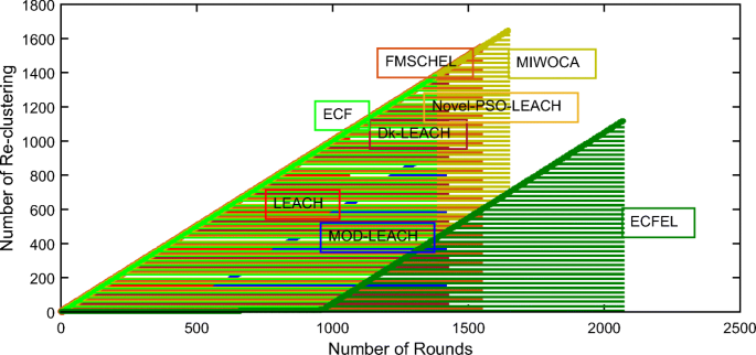
Number of times re-clustering is done for LEACH, MOD-LEACH, DkLEACH, Novel-PSO-LEACH, FM-SCHEL, M-IWOCA, ECF, and ECFEL
Fig. 9 
Energy consumption per round for LEACH, MOD-LEACH, DkLEACH, Novel-PSO-LEACH, FM-SCHEL, M-IWOCA, ECF, and ECFEL w.r.t. 50 devices
Fig. 10 
Energy consumption per round for LEACH, MOD-LEACH, DkLEACH, Novel-PSO-LEACH, FM-SCHEL, M-IWOCA, ECF, and ECFEL w.r.t. 100 devices
Fig. 11 
Energy consumption per round for LEACH, MOD-LEACH, DkLEACH, Novel-PSO-LEACH, FM-SCHEL, M-IWOCA, ECF, and ECFEL w.r.t. 1000 devices
- Packet Delivery Ratio (PDR): :
-
Fig. 14 represents the PDR. From the graph, it can be deduced that ECFEL comes out to be better than rest. From the graph in Fig. 14, we can see that LEACH, MOD-LEACH, DK-LEACH, Novel-PSO-LEACH, FM-SCHEL, M-IWOCA, ECF, and ECFEL are performing equally good up to 700-800 rounds, but in later rounds, ECFEL is outperforming comparably. The reason behind the drop-down after approximately 800 rounds w.r.t. all can be understood better from the Figs. 5, 6 and 7. We have seen that FND and HND has occurred before and after 800 rounds w.r.t. all. We know that with the time, energy will start decreasing as well, more devices started dying and hence PDR also started dropping. But the drop-rate in ECFEL is less in comparison to others which have a sharp fall after 1000 rounds. Because the key factors that can influence the energy consumption of sensors are taken into account. Major factors behind the energy consumption in IoT devices are as following: frequency of re-clustering, properties of each device considered for CHs selection, and the distribution of selected CHs. PDR for ECFEL is maintained high even when the network is scaled to 100 and 1000 devices which is not the case for MOD-LEACH, as depicted in Figs. 15 and 16. Now, if the lifetime of the network is specified as 50% PDR or more, ECFEL's network lifetime is better than others. The reason behind it is better CH selection by considering CH lifetime of devices and their spatial or geographic placement w.r.t. each other. Furthermore, from all of the above graphs, it is very much clear that the proposed technique doing efficiently for large scale networks as well. So, ECFEL ensures scalability, which is again one of the significant achievements of this approach, which is absent in MOD-LEACH, DkLEACH, and Novel-PSO-LEACH, FM-SCHEL, M-IWOCA techniques.


Uniform selection of CHs in proposed protocol [blue stars are sensor devices, red diamond are selected CHs and green star is sink]


Packet delivery ratio for LEACH, MOD-LEACH, DkLEACH, Novel-PSO-LEACH, FM-SCHEL, M-IWOCA, ECF, and ECFEL w.r.t. 50 devices

Packet delivery ratio for LEACH, MOD-LEACH, DkLEACH, Novel-PSO-LEACH, FM-SCHEL, M-IWOCA, ECF, and ECFEL w.r.t. 100 devices

Packet delivery ratio for LEACH, MOD-LEACH, DkLEACH, Novel-PSO-LEACH, FM-SCHEL, M-IWOCA, ECF, and ECFEL w.r.t. 1000 devices
6 Conclusion
In this paper, we presented the ECFEL protocol, which elongates the lifetime of WSNs assisted IoT. It is an improvement over M-IWOCA, FM-SCHEL, Novel-PSO-LEACH, MOD-LEACH, DkLEACH, and LEACH protocol. We have already estimated the lifetime of IoT devices as CHs by utilizing the linear optimization. In ECFEL, we have considered the node centrality, residual energy, and estimated the lifetime of a IoT device as a CH. We selected the CHs by using the chance of election value obtained using FLC. We have stalled the re-clustering process and hence minimized energy consumption. The comparison of ECFEL with M-IWOCA, FM-SCHEL, Novel-PSO-LEACH, MOD-LEACH, DkLEACH, and LEACH clearly favors the proposed protocol. To showcase the benefits provided by the parameter i.e. estimated lifetime of IoT devices as CH, we have passed only residual energy and node centrality parameters into fuzzy logic (ECF) and kept its results as well in the graphs. We have found that ECFEL outperforms M-IWOCA, FM-SCHEL, Novel-PSO-LEACH, MOD-LEACH, DkLEACH, and LEACH. It enhances the network lifetime, balances the energy consumption, and improves packets delivered to the sink. The results have also shown that the proposed approach is an excellent choice for large scale networks.
However, the computation required to estimate the novel parameter may lead to high computational complexity. Along with it, there is a requirement of hardware and software which provide a precise estimation. In future, soft computing techniques can be utilized to estimate the lifetime of IoT devices as CHs and CMs to reduce the complexity. CHs selection on IoT based on different attributes can also be explored further. Thereafter, multi-path routing can be further incorporated to minimize energy consumption.
References
Ahmad A, Ahmed S, Imran M, Alam M, Niaz IA, Javaid N (2017) On energy efficiency in underwater wireless sensor networks with cooperative routing. Ann Telecommun 72(3-4):173–188
Asghari P, Rahmani AM, Javadi HHS (2019) Internet of things applications: a systematic review. Comput Netw 148:241–261
Bagci H, Yazici A (2010) An energy aware fuzzy unequal clustering algorithm for wireless sensor networks. In: International conference on fuzzy systems, IEEE, pp 1–8
Dhumane AV, Prasad RS (2019) Multi-objective fractional gravitational search algorithm for energy efficient routing in iot. Wireless Netw 25(1):399–413
Din S, Ahmad A, Paul A, Rathore MMU, Jeon G (2017) A cluster-based data fusion technique to analyze big data in wireless multi-sensor system. IEEE Access 5:5069–5083
Ding X-X, Ling M, Wang Z-J, Song F-L (2017) Dk-leach: an optimized cluster structure routing method based on leach in wireless sensor networks. Wirel Pers Commun 96(4):6369–6379
Falcon R, Jeon G, Bello R, Jeong J (2007) Learning collaboration links in a collaborative fuzzy clustering environment. In: Mexican international conference on artificial intelligence, Springer, pp 483– 495
Farahani M, Rahbar AG (2019) Double leveled unequal clustering with considering energy efficiency and load balancing in dense iot networks. Wirel Pers Commun 106(3):1183–1207
Haseeb K, Lee S, Jeon G (2020) Ebds: An energy-efficient big data-based secure framework using internet of things for green environment. Environmental Technology & Innovation, pp 101129
Heinzelman WR, Chandrakasan A, Balakrishnan H (2000) Energy-efficient communication protocol for wireless microsensor networks. In: Proceedings of the 33rd annual Hawaii international conference on system sciences, IEEE, pp 10–pp
Huang J, Ruan D, Meng W (2018) An annulus sector grid aided energy-efficient multi-hop routing protocol for wireless sensor networks. Comput Netw 147:38–48
Hussain F, Hussain R, Hassan SA, Hossain E (2020) Machine learning in iot security: current solutions and future challenges. IEEE Communications Surveys & Tutorials
Jianyin L (2012) Simulation of improved routing protocols leach of wireless sensor network. In: 2012 7Th international conference on computer science & education (ICCSE), IEEE, pp 662–666
Lee J-S, Cheng W-L (2012) Fuzzy-logic-based clustering approach for wireless sensor networks using energy predication. IEEE Sensors J 12(9):2891–2897
Li J, Silva BN, Diyan M, Cao Z, Han K (2018) A clustering based routing algorithm in iot aware wireless mesh networks. Sustainable Cities and Society 40:657–666
Lin J, Duan G, Tian Z (2020) Interval intuitionistic fuzzy clustering algorithm based on symmetric information entropy. Symmetry 12(1):79
Lin D, Wang Q, Min W, Jianfeng X u, Zhang Z (2020) A survey on energy-efficient strategies in static wireless sensor networks. ACM Transactions on Sensor Networks (TOSN) 17(1):1–48
Liu X, Fu L, Wang J, Wang X, Chen G (2019) Multicast scaling of capacity and energy efficiency in heterogeneous wireless sensor networks. ACM Transactions on Sensor Networks (TOSN) 15(3):1–32
Logambigai R, Kannan A (2016) Fuzzy logic based unequal clustering for wireless sensor networks. Wirel Netw 22(3):945–957
Mahmood D, Javaid N, Mahmood S, Qureshi S, Memon AM, Zaman T (2013) Modleach: a variant of leach for wsns. In: 2013 Eighth international conference on broadband and wireless computing, communication and applications, IEEE, pp 158–163
Majadi N, Mahmud SR, Sultana M (2013) Uniform distribution technique of cluster heads in leach protocol. International Journal on Recent Trends in Engineering & Technology 8(1):84
Maratha P et al (2019) A comparative study on prominent strategies of cluster head selection in wireless sensor networks. In: Integrated intelligent computing, communication and security, Springer, pp 373–384
Mirzaie M, Mazinani SM (2017) Adaptive mcfl: an adaptive multi-clustering algorithm using fuzzy logic in wireless sensor network. Comput Commun 111:56–67
Orlin J (2013) LP Transformation techniques. Spring
Pourghebleh B, Hayyolalam V (2019) A comprehensive and systematic review of the load balancing mechanisms in the internet of things. Clust Comput, pp 1–21
Qureshi KN, Tayyab MQ, Rehman SU, Jeon G (2020) An interference aware energy efficient data transmission approach for smart cities healthcare systems. Sustainable Cities and Society 62:102392
Rostami AS, Badkoobe M, Mohanna F, Hosseinabadi AAR, Sangaiah AK et al (2018) Survey on clustering in heterogeneous and homogeneous wireless sensor networks. J Supercomput 74(1):277–323
Sathya Lakshmi Preeth SK, Dhanalakshmi R, Kumar R, Mohamed Shakeel P (2018) An adaptive fuzzy rule based energy efficient clustering and immune-inspired routing protocol for wsn-assisted iot system. Journal of Ambient Intelligence and Humanized Computing, pp 1–13
Sert SA, Bagci H, Yazici A (2015) Mofca: Multi-objective fuzzy clustering algorithm for wireless sensor networks. Appl Soft Comput 30:151–165
Shahraki A, Taherkordi A, Haugen Ø, Eliassen F (2020) Clustering objectives in wireless sensor networks: a survey and research direction analysis. Comput Netw 180:107376
Sharma R, Vashisht V, Singh U (2019) Fuzzy modelling based energy aware clustering in wireless sensor networks using modified invasive weed optimization. Journal of King Saud University-Computer and Information Sciences
Singh AK, Purohit N, Varma S (2013) Fuzzy logic based clustering in wireless sensor networks: a survey. Int J Electron 100(1):126–141
Souri A, Hussien A, Hoseyninezhad M, Norouzi M (2019) A systematic review of iot communication strategies for an efficient smart environment. Transactions on Emerging Telecommunications Technologies, pp e3736
Sreenivasamurthy S, Obraczka K (2018) Clustering for load balancing and energy efficiency in iot applications. In: 2018 IEEE 26Th international symposium on modeling, analysis, and simulation of computer and telecommunication systems (MASCOTS), IEEE, pp 319–332
Sung Y, Lee S, Lee M (2018) A multi-hop clustering mechanism for scalable iot networks. Sensors 18(4):961
Thiagarajan R et al (2020) Energy consumption and network connectivity based on novel-leach-pos protocol networks. Comput Commun 149:90–98
Ullah MF, Imtiaz J, Maqbool KQ (2019) Enhanced three layer hybrid clustering mechanism for energy efficient routing in iot. Sensors 19(4):829
Uma Maheswari D, Sudha S (2019) Node degree based energy efficient two-level clustering for wireless sensor networks. Wirel Pers Commun 104 (3):1209–1225
Wazid M, Das AK, Hussain R, Succi G, Rodrigues JJPC (2019) Authentication in cloud-driven iot-based big data environment: survey and outlook. J Syst Archit 97:185–196
Xu X, Ansari R, Khokhar A, Vasilakos AV (2015) Hierarchical data aggregation using compressive sensing (hdacs) in wsns. ACM Transactions on Sensor Networks (TOSN) 11(3):1–25
Xu L, Collier R, O’Hare GMP (2017) A survey of clustering techniques in wsns and consideration of the challenges of applying such to 5g iot scenarios. IEEE Internet Things J. 4(5):1229–1249
Xu Y, Yue Z, Lv L (2019) Clustering routing algorithm and simulation of internet of things perception layer based on energy balance. IEEE Access 7:145667–145676
Acknowledgments
We thank Ashish Kumar Luhach from The PNG University of Technology, Papua New Guinea and Arnab Chakroborty from the Indian Statistical Institute, Kolkata for their constructive ideas and insightful discussion on improving the outlook of the paper. Priti Maratha, as part of the National Eligibility Test-Junior Research Fellowship scheme with Reference ID- 3361/(NET-JUNE 2015), acknowledges the assistance from University Grant Commission, New Delhi.
Author information
Authors and Affiliations
Corresponding author
Additional information
Publisher’s note
Springer Nature remains neutral with regard to jurisdictional claims in published maps and institutional affiliations.
Rights and permissions
About this article

Cite this article
Maratha, P., Gupta, K. Linear optimization and fuzzy-based clustering for WSNs assisted internet of things. Multimed Tools Appl 82, 5161–5185 (2023). https://doi.org/10.1007/s11042-021-11850-8
Received:
Revised:
Accepted:
Published:
Issue Date:
DOI: https://doi.org/10.1007/s11042-021-11850-8