Performance Analysis of the Industrial Wireless Networks Standard: WIA-PA

Abstract

This paper analyzes salient features of Industrial Automation-Process Automation (WIA-PA): mesh-star architecture, two-level aggregation, and adaptive frequency hopping, whose working principles are explicitly illustrated in comparison to the other two mainstream industrial wireless networks standards: WirelessHART and ISA 100.11a. In addition, performance analysis with respect to the three features of WIA-PA has been conducted in terms of communication overhead or transmission reliability. Our results demonstrate the performance advantages of WIA-PA over WirelessHART and ISA 100.11a.

1 Introduction

Advances in the technology and reduction of wireless communication cost have allowed multi-hop wireless networks to be used as a means of monitoring of large-scale industrial plants in process automation. With the advance of industrial wireless technologies, sensor measurements of plant variables can be transmitted to data centers without the need for excessive wiring, thereby yielding gains in efficiency and flexibility for the operator [1–4]. On the other hand, wireless technologies suffer from the harsh industrial environments since wireless channels are extremely prone to severe damage due to the coexisting interference, fading, and multi-path effect [5, 7]. Therefore, guaranteeing the deterministic requirement on the industrial wireless network in spite of the unfriendly wireless channel turns out to be a challenging problem, and industrial wireless networks (IWNs) have aroused a great deal of interest from academia [8–21], industry [22–24] as well as standardized organizations [25–27]. This paper aims to study IWNs from the standpoint of IWNs standards.

Wireless networks for Industrial Automation-Process Automation (WIA-PA) is one of the two only existing International Electrical Commission (IEC) standards, and was initialized by the Chinese Industrial Wireless Alliance (CIWA) in August 2008 and finally approved by the IEC in October 2011. In order to meet the stringent demand by industrial monitoring and control applications, such as low real-time latency bound, high transmission reliability, and longevity, WIA-PA favors the mesh-star architecture, and supports the two-level aggregation and adaptive frequency hopping (AFH). Specifically, as shown in Fig. 1, the mesh-star architecture is a hierarchical network architecture, whose first level is the mesh topology where routing devices form a mesh, and its second level is in star topology, also termed a cluster, where routing devices act as cluster heads and field devices as cluster members. The mesh-star architecture will be shown to reduce communication overhead for both the flooding and the unicast cases. The two-level aggregation including data aggregation at the application layer and packet aggregation at the network layer is proposed to reduce the redundancy in data transmission for high energy efficiency. AFH is employed to combat erroneous wireless channels for high transmission reliability. In the this paper, each of the aforementioned features will be illustrated in details and the advantages of WIA-PA over other IWNs standards will also be examined by theoretical analysis. To the best of our knowledge, this paper serves as the first theoretical contribution to the performance analysis of WIA-PA, and this work will promote the development of WIA-PA and extend its applications in the industrial field.

Fig. 1

WIA-PA network topology (mesh-star architecture)[27]

The rest of this paper is organized as follows. In Section 2, related IWNs standards are reviewed. Section 3 conducts theoretical analysis on the novel features of WIA-PA. Section 4 discusses open directions for future research in WIA-PA networks. Section 5 finally concludes this paper.

2 Related work

This section will present an overview of the three mainstream IWNs standards (i.e., WirelessHART [25], ISA 100.11a [26], and WIA-PA [27]) that have been specifically tailored for usage in industrial process automation, in which comparisons of technical differences of three standards are especially illustrated.

The Highway Addressable Remote Transducer (HART) Communication Foundation (HCF) released the HART Field Communication Protocol Specification in September 2007, referred to as WirelessHART, which is the first open and interoperable international WSN standard specifically designed to address industrial process automation. The International Society of Automation (ISA) initiated work on a family of standards defining wireless systems for industrial automation and control applications. The first standard to emerge was ISA 100.11a, which was ratified as an ISA standard in September 2009 and aimed to provide secure and reliable wireless solution for noncritical monitoring and control applications. Parallel to the development of HCF and ISA, in 2007, the Chinese Industrial Wireless Alliance (CIWA) was founded by Shenyang Institute of Automation, Chinese Academy of Sciences as well as other ten universities, academies, and industrial companies in China. WIA-PA was proposed to serve as the wireless solution to industrial process automation and became the second IEC standard of industrial wireless networks in 2012.

Some related works for WIA-PA are listed as follows. The paper [12] provides a survey of WIA-PA, compares it with WirelessHART and ISA100.11a, and presents some experiment results of WIA-PA. The paper [13] shows how WIA-PA interconnects with legacy process automation system. The paper [16] proposes a asynchronous multi-channel neighbor discovery method for time division multiple access (TDMA) for WIA-PA. The paper [17] studies a collision-free multichannel superframe scheduling problem for WIA-PA. The paper [18] presents a frequency domain polling MAC protocol for WIA-PA. The paper [19] studies random time source protocol for WIA-PA.

This paper highlights three selected features of WIA-PA and makes a comparison between WIA-PA and other two mainstream IWNs standards (shown in Table 1), where comprehensive comparison of the three IWNs standards can be found in [12]. Specifically, from the perspective of network architecture, both the star and mesh architectures are supported by ISA 100.11a and WirelessHART, but only the mesh architecture is recommended. In contrast, WIA-PA favors the mesh-star architecture rather than the mesh architecture; from the perspective of system management, WIA-PA supports two-level aggregation (i.e., data aggregation at the application layer and packet aggregation at the network layer), while ISA 100.11a and WirelesHART only support data aggregation function; from the perspective of frequency hopping technology, WIA-PA adopts AFH that only changes the working frequency when interference is detected on the operating channel. Different from WIA-PA, both WirelessHART and ISA 100.11a adopt the blind frequency hopping (BFH) with or without whitelisting, which inefficiently hops over all possible channels without considering channel variations according to a pseudo-random sequence.

Table 1 Comparison results on selected features of existing IWNs standards

3 Performance analysis

3.1 System architecture

The WIA-PA network mainly employs the two-level hybrid network architecture in which the first level forms a mesh and the second level consists of a group of clusters. In the following, we will demonstrate the advantages of two-level hybrid network architecture (WIA-PA) over the pure mesh architecture (WirelessHART and ISA 100.11a) in terms of communication overhead.

Network scenario

Consider a mesh network with one gateway, h hops and N _i (1 ≤ i ≤ h) nodes at hop i (shown in Fig. 2). Thus, the number of sensor nodes in the network could be calculated as N = N ₁ + N ₂ + … + N _h . In comparison to the mesh network, the mesh-star network also takes routing devices into account. Similarly suppose that the mesh level of the mesh-star network is with one gateway, h ^′ hops and $N_{i}^{\prime }(1\leq i\leq h^{\prime })$ routers labeled as $1,2, ..., N_{i}^{\prime }$ at hop i (shown in Fig. 3), and denote $N^{\prime }=N_{1}^{\prime }+N_{2}^{\prime }+\ldots +N_{h^{\prime }}^{\prime }$ the number of routers in the mesh-star network. Each cluster at (i, j) consists of one routing device¹

Fig. 2

Mesh network mainly employed by WirelessHART and ISA 100.11a

Fig. 3

Mesh-star network mainly employed by WIA-PA

and n _{i j} (n _{i j} ≥ 0) associated sensor nodes, where pair (i, j) denotes the ID of the jth cluster at hop i.

For fair comparison, assume that the quantities of sensors for both network architectures are equal, i.e., $N={\sum }_{i=1}^{h^{\prime }}{\sum }_{j=1}^{N_{i}^{\prime }}n_{ij}$ and both mesh-level networks employ the same routing algorithm. Without loss of generality, the minimum hop routing algorithm is employed throughout this paper, and the minimum hop routing algorithm is performed at the gateway and lies in the scope of graph routing that is widely adopted by IWNs. In this section, we will only study the downlink case where data originates from the gateway and is transmitted to the sensors. For ease of analysis, error-free communication is assumed. The following analysis will be done for two representative communication patterns in IWNs.

(1) Flooding: Network flooding has been investigated extensively for network-wide dissemination of commands, configurations, and code binaries in WSNs, and has been formed the basis for a wide range of network operations, such as routing and time synchronization. In order to allow complete information update within the network, for a mesh network, apart from the nodes at hop h, each other node in the network only has to carry out one broadcast (i.e., only the first received broadcast message is rebroadcast and other outdated messages at each node are discarded), while for a star-mesh network, only router devices conduct broadcast. Consequently, the number of needed transmissions for the mesh network ($N_{F_{m}}$) and the mesh-star network ($N_{F_{ms}}$), termed hereafter as communication overhead, can be calculated as follows:

$$ N_{F_{m}}=1+N_{1}+N_{2}+\ldots+N_{h-1}=N+1-N_{h}=\mathcal{O}(N) $$

(1)

and

$$\begin{array}{@{}rcl@{}} N_{F_{ms}}&=\underbrace{1+N_{1}^{\prime}+N_{2}^{\prime}+\ldots+N_{h^{\prime}-1}^{\prime}}_{mesh}+\underbrace{N_{1}^{\prime}+N_{2}^{\prime}+\ldots+N_{h^{\prime}}^{\prime}}_{star} \\ &=2N^{\prime}+1-N_{h^{\prime}}=\mathcal{O}(N^{\prime}). \end{array} $$

(2)

Note that the processing overhead for those overheard packets during flooding is neglected when calculating the communication overhead, and this is reasonable since communications usually dominate the energy consumption and the delay of wireless transceivers.

(2) Unicast: Unicast mainly happens when the network manager configures ID, address, and routes for each node during the network initialization period. For a mesh network, the number of transmissions for updating nodes at hop i is i N _i , and thus the communication overhead of unicast in the mesh network $N_{U_{m}}$ is given by

$$ N_{U_{m}}=N_{1}+2N_{2}+\ldots+hN_{h}=\mathcal{O}(h^{2}N). $$

(3)

In contrast, the mesh-star network takes advantages of the distributed management function of cluster heads [27] to reduce the unnecessary communication. Specifically, the information distribution process in the mesh level of the mesh-star network is the same as that in the mesh network, while in the cluster level, each cluster head abstracts the cluster resource information (e.g., time slots and channels) allocated by the Gateway and distributes the configuration information to its associated cluster members via unicast. In other words, for each cluster (i, j), n _{i j} transmissions are needed. As a result, we have the communication overhead of unicast in the mesh-star network

$$\begin{array}{@{}rcl@{}} N_{U_{ms}}&=&\underbrace{N_{1}^{\prime}+2N_{2}^{\prime}+\ldots+h^{\prime}N_{h^{\prime}}^{\prime}}_{mesh}+\underbrace{\sum\limits_{i=1}^{h^{\prime}}\sum\limits_{j=1}^{N_{i}^{\prime}}n_{ij}}_{star} \\ &=&N_{1}^{\prime}+2N_{2}^{\prime}+\ldots+h^{\prime}N_{h^{\prime}}^{\prime}+N \\ &=&\left\{\begin{array}{l} \mathcal{O}(N), \quad \quad \quad \ if \ (h^{\prime})^{2}N^{\prime}= \mathcal{O}(N) \\ \mathcal{O}((h^{\prime})^{2}N^{\prime}), \quad if \ N= \mathcal{O}((h^{\prime})^{2}N^{\prime}) \end{array}\right. \end{array} $$

(4)

From Eqs. 1 and 4, we conclude that as shown in Table 2, both $N_{U_{I}}$ and $N_{F_{I}} (I\in \{m,ms\})$ completely depend on the scale of the mesh topology (formed by sensors in the mesh network, while by devices in the mesh-star network). Observed from Table 2, as the number of routing devices is normally far less than that of sensors, the mesh-star network will achieve considerable overhead saving in comparison to the mesh network, especially when unicast communication is considered.

Table 2 Communication overhead Comparison between mesh and mesh-star architectures

Comment 1: :

No requirement on clustering algorithms of WIA-PA network is imposed in this paper, and this means that the above communication overhead analysis will continue to hold for any clustering scheme.

Comment 2: :

In practice, convergecast communication that periodically collects data from sensors to gateway dominates the uplink communication. With respect to convergecast, the mesh-star architecture is with the same order of communication overhead as the mesh architecture; however, the mesh-star architecture adopts two-level aggregation which will help reduce energy consumption shown in Section 3.2.

3.2 Aggregation function

Two-level aggregation is another feature of WIA-PA, since ISA 100.11a and WirelessHART only support one-level aggregation, i.e., data aggregation. It is well-known that aggregation allows combining multiple small packets into large ones and thus reduces unnecessary overhead due to packet headers [28–31]. This subsection will show how many bits and packets can be saved by the two-level aggregation.

Consider a WIA-PA network with one gateway, h levels (hops) of routing devices, with R _i (1 ≤ i ≤ h) routers at hop i and n _{i j} sensors in cluster (i, j). Taking cluster (i, j) as an example, we label its cluster members as F _{i j t} (0 ≤ t ≤ n _{i j} ), where F _{i j0} represents the head of cluster (i, j). Sensor F _{i j t} will periodically report to the Gateway via F _{i j0}. Suppose that the data packet of F _{i j t} is with the size l _{i j t} , l _{i j t} = H+d _{i j t} , where H denotes the length of packet header (that is specified by WIA-PA) and d _{i j t} the payload size of sensor t in cluster (i, j).

• 1) Packet Aggregation: Packet aggregation is employed by cluster head to reduce the transmitted bits. Before packet aggregation, we have the number of bits produced by cluster (i, j)

  $$ B_{ij}=\sum\limits_{t=1}^{n_{ij}}l_{ijt}I_{ijt} $$

  (5)

  where Boolean indicator I _{i j t} = 1 if sensor F _{i j t} has data to transmit, and I _{i j t} = 0 otherwise (Fig. 4).

  Fig. 4

  

  Illustration on the process of packet aggregation

  Then we continue to calculate the amount of bits at F _{i j0} after packet aggregation, which is equivalent to the following problem ($\mathcal {P}$): How many bits in total are needed by packet aggregation to guarantee the delivery of payload in Cluster (i, j)? Obviously, at least the size of payload, ${\sum }_{t=1}^{n_{ij}}d_{ijt} I_{ijt}$, should be counted. Consequently, problem $\mathcal {P}$ reduces to the calculation of the total packet header cost, i.e., the number of packets (since H bits per header is specified). Let L (L > H) denote the maximum length of each packet, then we need N _{P, i j} packets to pack the payload

  $$ N_{P,ij}=\left\lceil \frac{{\sum}_{t=1}^{n_{ij}}d_{ijt} I_{ijt}} {L-H} \right \rceil $$

  (6)

  where all packets except the last one are maximum sized, and the number of these maximum sized packets, denoted as N _{P−m a x, i j} , is given by

  $$ N_{P-max,ij}=\left\lfloor \frac{{\sum}_{t=1}^{n_{ij}}d_{ijt} I_{ijt}} {L-H} \right \rfloor $$

  (7)

  where ⌈⋅⌉ and ⌊⋅⌋ represent the Ceiling and the Floor functions, respectively.

  Base on the above analysis, after packet aggregation the total number of bit at F _{i j0} will therefore be

  $$ A_{ij}=N_{P,ij}H+ \sum\limits_{t=1}^{n_{ij}}d_{ijt} I_{ijt} . $$

  (8)

• 2) Data aggregation: Most of the current commercial sensors off the shelf can sense multiple physical parameters, such as pressure, temperature, humidity, etc. In the multi-object case, data aggregation can further reduce the bits cost due to the application layer header, by combining multiple small application layer data packets for different physical observations into large ones.

  We shall note that the principles in Eqs. 5 and 8 are perfectly applicable to the analysis of data aggregation if sensor nodes and separate objects in data aggregation are compared to cluster heads and sensors in packet aggregation (shown in Fig. 5), respectively. Therefore, we just skip the analysis for data aggregation and for ease of exposition we assume that application layer packets after data aggregation remain not maximum sized. For the rest of this paper, we continue to use notation d _{i j t} to represent the length of application layer packet (i.e., network layer payload) after data aggregation, at sensor t in cluster (i, j).

  Fig. 5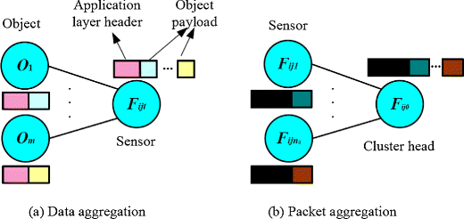

  

  Similarity between data aggregation and packet aggregation

• 3) Retransmission The industrial communication is inherently one classification of machine-to-machine (M2M) communications [32, 33], in which packets are commonly very small. Therefore, the reasonability of the error-free assumption holds for the small packets communication. However, the increase of packet length due to the two-level aggregation will lead the increase of the packet error rate at the receiver side. In this paper, transmission error rate p(l) is modeled as the function of packet length l. In order to characterize the dependency between packet length and packet error rate, we made the experiment shown in Fig. 6. The experiment setup that we consider comprises two nodes, S ₁ (transmitter) and S ₂ (receiver), that communicate over an unlicensed channel. For each different packet length (10, 20, 30, …, 60 bytes), S ₁ sends one packet to S ₂ every 500ms until the number of transmitted packets reaches 10⁴. The S ₂ then calculates the error rate (including bit error and packet loss) based on the achieved statistical data. Notice that in order to avoid noisy factors, the experiment was done in an obstacle-free anechoic chamber.

  Fig. 6

  

  Experiment setup

  The experimental results are depicted in Fig. 7 and each point in Fig. 7 is averaged over 10⁴ packets. Fig. 7 indicates that error rate is a monotonic increasing function of packet length and the increasing rate grows fairly rapid at the large size period. As shown in Fig. 7, the curve looks like the right branch of a quadratic function. Error-free assumption obviously does not hold in the case of large packets, for which we consider retransmissions performed by some Automatic ReQuest (ARQ) protocols at link level to compensate for transmission errors. As a result, the average number of transmissions $\hat {n}$ required over each hop to reliably transmit a packet with length l is given by $\frac {1}{1-p(l)}$.

  Fig. 7

  

  Error rate as a function of packet length

  Finally, considering the WIA-PA network topology under investigation and summing over all clusters, we finally achieve the effective number of the totally needed bits A _{n e t}

  $$ A_{net}=\sum\limits_{i=1}^{h} \sum\limits_{j=1}^{R_{i}}i\left(\frac{L\times N_{P-max,ij}}{1-p(L)}+\frac{{\Omega}_{ij}}{1-p({\Omega}_{ij})}\right) $$

  (9)

  where Ω _{i j} = A _{i j} − L × N _{P−m a x, i j} denotes the length of the unique unsaturated packet at F _{i j0}.

  With Eqs. 5 and 9 in hand, the number of ’saved bits’ △ _{n e t} is given by

  $$ \triangle_{net}=\sum\limits_{i=1}^{h} \sum\limits_{j=1}^{R_{i}}iB_{ij}-A_{net}=\sum\limits_{i=1}^{h} \sum\limits_{j=1}^{R_{i}}i\triangle_{ij} $$

  (10)

  where $\triangle _{ij}=B_{ij}-\frac {L\times N_{P-max,ij}}{1-p(L)}-\frac {{\Omega }_{ij}}{1-p({\Omega }_{ij})}$.

  When the maximum length of packet L is small (e.g., L ≤ 40 bytes), the error rate in Fig. 7 is so small that the error-free assumption holds reasonably. Then, △ _{i j} could be approximated as follows:

  $$\begin{array}{@{}rcl@{}} \triangle_{ij} &\approx B_{ij}-L\times N_{P-max,ij}-{\Omega}_{ij} \\ &=B_{ij}-A_{ij} \\ &=\left(\left\lceil \frac{{\sum}_{t=1}^{n_{ij}}d_{ijt} I_{ijt}} {L-H} \right \rceil-n_{ij} \right)H \end{array} $$

  (11)

  As parameters L, H and n _{i j} in Eq. 11 are fixed, it is obvious that △ _{i j} only depends on the size of payload. Specifically,

  $$ \triangle_{ij} \left\{\begin{array}{l} >0, \quad {\sum}_{t=1}^{n_{ij}}d_{ijt} I_{ijt} <(n_{ij}-1)(L-H)\\ =0, \quad (n_{ij}-1)(L-H)\leq {\sum}_{t=1}^{n_{ij}}d_{ijt} I_{ijt} <n_{ij}(L-H). \\ \end{array} \right. $$

  (12)

  Equation 12 tells us that two-level aggregation will always yield bits saving except for some special cases, e.g., original packets of sensors are almost all maximum sized.

  However, in case of large L (e.g., L ≥ 50 bytes in Fig. 7), the advantage of aggregation function becomes diminishing, and thus the revaluation of Eq. 10 is needed. Due to the lack of an analytical expression for p(l), the sign of △ _{i j} only can be judged in a numerical way. To avoid the complex revaluation process, we do not recommend the use of large L in practice.

• 4.) Saved packets by packet aggregation

  As data aggregation function is supported by WIA-PA, WirelessHART, and ISA 100.11a, this subsection needs only to compare the overhead of convergecast communication for two cases, i.e., with packet aggregation (WIA-PA) and without packet aggregation (WirelessHART and ISA 100.11a).

  Obviously, in one convergecast period the number of original packets in WirelessHART or ISA 100.11a networks is given by

  $$ N_{WP}=\sum\limits_{i=1}^{h} \sum\limits_{j=1}^{R_{i}}\sum\limits_{t=1}^{n_{ij}}I_{ijt}. $$

  (13)

  While for WIA-PA networks, we know that from Eq. 7 the number of aggregated packets at cluster head F _{i j0} is N _{P, i j} , and thus the number of aggregated packets at the mesh-level of WIA-PA networks is as follows:

  $$ N_{WPA}=\sum\limits_{i=1}^{h} \sum\limits_{j=1}^{R_{i}}\left\lceil \frac{{\sum}_{t=1}^{n_{ij}}d_{ijt}I_{ijt}}{L-H}\right\rceil. $$

  (14)

  It is straightforward to show that

  $$\begin{array}{@{}rcl@{}} N_{WP}-N_{WPA}&={\sum}_{i=1}^{h} {\sum}_{j=1}^{R_{i}}\left\{{\sum}_{t=1}^{n_{ij}}I_{ijt}-\left\lceil {\sum}_{t=1}^{n_{ij}}\frac{d_{ijt}I_{ijt}}{L-H}\right\rceil\right\} \\ &\geq_{a} {\sum}_{i=1}^{h} {\sum}_{j=1}^{R_{i}}\left\{{\sum}_{t=1}^{n_{ij}}I_{ijt}-\left\lceil {\sum}_{t=1}^{n_{ij}}I_{ijt}\right\rceil\right\} \\ &=0 \end{array} $$

  (15)

  where “ ≥ _a ” follows from $\frac {d_{ijt}}{L-H}\leq 1$, ∀i, j, t, and N _{W P} = N _{W P A} holds if and only if $0\leq {\sum }_{t=1}^{n_{ij}}\left (1-\frac {d_{ijt}}{L-H}\right )I_{ijt}<1$. Similar to Eq. 11, the number of the ’saved’ packets (the gap between N _{W P} and N _{W P A} ) depends on the payload size ${\sum }_{t=1}^{n_{ij}}d_{ijt}I_{ijt}$, ∀i, j.

3.3 Frequency hopping

Frequency hopping, as a class of frequency diverse communication protocols, has been commonly used as a method for IWNs to enable sharing of the 2.4GHz Industrial, Scientific and Medical (ISM) band with other proximate networks, such as IEEE 802.11b/g networks, Bluetooth networks, etc [34, 35]. Both blind frequency hopping (BFH) and adaptive frequency hopping (AFH) are widely used frequency hopping techniques by IWNs, where the former is favored by the WirelessHART and ISA 100.11a [25, 26] and the latter by WIA-PA [27, 40].

With BFH each node uniformly hops over all 16 channels of 2.4GHz ISM band. Whitelisting is an advanced variant of BFH, in which two neighbor nodes agree upon a subset of the available channels and hop only over that subset of channels. The disadvantage of BFH is the ’blindness’, i.e., nodes simply hop over some subsets of channels according to some Pseudo-random channel sequence, regardless of the current state of the operating channel. Suppose that one node switches from a good channel to a congested one, and then this hopping will produce interference instead of mitigating interference. In contrast, AFH allows nodes to choose working channels according to the historical statistics of channel state. Obviously, an effective AFH will help to reduce the probability of inefficient hopping, e.g., switches from good channels to bad channels.

As we know, aside from collision, IEEE 802.11b/g networks is the main interferer to IWNs [36–38]. There are two reasons. First, the transmission power of IEEE 802.11b/g devices is much higher than that of IEEE 802.15.4 devices, and this means the transmission of IWNs devices will fail as long as other collocated IEEE 802.11b/g devices are working on the same channel. Second, IEEE 802.11b/g and IEEE 802.15.4 channels are highly overlapped. Specifically, as shown in Fig. 8, we observe that channels are completely dominated by the IEEE 802.11b/g networks except for four channels (channel 15, 20, 25, and 26). However, restricting the number of available channels (e.g., the four interference-free channels) may not be an efficient way to mitigate interference form other sources and in fact increases the chance that collocated IWNs will interfere with each other.

Fig. 8

IEEE 802.11b/g and IEEE 802.15.4 channel overlap

To illustrate the power of AFH approaches, in this section we propose a simple strategy that is able to dynamically switch the channel on which nodes communicate, and use as many channels as possible, even in the presence of active IEEE 802.11b/g devices. Let $\mathcal {F}:=\{11, 12,\ldots , 26\}$ denote the channel set, i.e., the set of all 16 available channels of IEEE 802.15.4 over which AFH is applied. Each element $i \in \mathcal {F}$ uniquely corresponds to one channel in 2.4GHz ISM band. For ease of presentation, we denote the three overlapping channels of IEEE 802.11b/g networks in Fig. 8 as C _a ({11, 12, 13, 14}), C _b ({16,17,18,19}), and C _c ({21,22,23,24}), respectively. Motivated by the fact that the channel C _I (∀I ∈ {a, b, c}) is unavailable once IEEE 802.11b/g interference is detected on any channel within C _I , we conclude the rational of our strategy, i.e., jumping out of the channel set that is occupied by active IEEE 802.11 devices. Let c _o and c _n ($c_{o}, c_{n} \in \mathcal {F}$) denote the ID of the current operating channel and the next working channel, respectively. Mathematically, c _n could be calculated if channel c _o is detected unavailable

$$ c_{n}= c_{o}\oplus S_{o} $$

(16)

where ⊕ is addition modulo 16, and integer S _o (1 ≤ S _o ≤ 15) represents the hopsize of frequency hopping. In addition, the choice of S _o is subject to the following condition:

$$ c_{o}\oplus S_{o}\notin C_{I} $$

(17)

if c _o ∈ C _I holds for some I ∈ {a, b, c}. Obviously, due to the fixed cardinality of each C _I (|C _I | = 4), I∈{a, b, c}, any S _o ∈ {4, 5, 6, ..., 15} will satisfy condition Eq. 17.

Let us consider a concrete example. Suppose a pair of WIA-PA nodes are communicating on channel c _o and IEEE 802.11b/g devices then start to work on this channel. For simplicity, here we set S _o = 5 for any starting channel c _o . Next, we discuss the calculation of c _n under different representative settings. Let $\mathcal {I}(C_{a})=1$ denote the case that channel C _a is occupied by IEEE 802.11b/g network, and $\mathcal {I}(C_{a})=0$ otherwise.

Case 1: c _o = 11, $\mathcal {I}(C_{a})=1$, $\mathcal {I}(C_{b})=0$, $\mathcal {I}(C_{c})=0$:

$$c_{n}= 11\oplus 5=16 $$

Notice that $c_{n}\in \mathcal {I}(C_{b})$ together with $\mathcal {I}(C_{b})=0$ implies the successful transmission of this frequency hopping.

Case 2: c _o = 17, $\mathcal {I}(C_{a})=0$, $\mathcal {I}(C_{b})=1$, $\mathcal {I}(C_{c})=1$:

$$c_{n}(1)= 17\oplus 5=22, c_{n}=c_{n}(1)\oplus 5=11 $$

where c _n (1) representing the ID of the first hopping channel lies in the unavailable set C _c , and this implies the failure of the first hopping. However, the second frequency hopping c _n = 11 is successful, since $c_{n}\in \mathcal {I}(C_{a})$ and $\mathcal {I}(C_{a})=0$ hold at the same time.

If the channel state is time-invariant during a long observation period, we can simply calculate the transmission reliability p _i of BFH for Case i (i = 1, 2),

$$ p_{i}=\frac{4\times{\sum}_{I\in \{a,b,c\}}\mathcal{I}(C_{I})}{16}=\frac{{\sum}_{I\in \{a,b,c\}}\mathcal{I}(C_{I})}{4}, $$

(18)

i.e., p ₁ = 75 % and p ₂ = 50 %, while the proposed AFH algorithm Eqs. 16 and 17 nearly guarantees 100 % transmission reliability.

However, the assumption of time-invariant channel over a long period is impractical. In the rest of this paper, assuming that each C _I (I ∈ {a, b, c}) independently follows a Bernoulli process, we compare AFH with BFH in terms of transmission reliability through simulation. Specifically, in each time slot, each C _I is available with probability p _I and unavailable 1−p _I . In the simulation, we assume that all p _I s are equal, i.e., p _I = p. Fig. 9 shows the comparison results between AFH and BFH for p ∈ [0.1, 0.9]. For each given p, 10⁴ successive time slots are observed and transmission reliability is defined as the ratio of the number of transmission failures to the number of total transmissions (10⁴). For fair comparisons, an arbitrarily chosen c ₀ is used for both AFH and BFH, and each of those four channels unoccupied by IEEE 802.11 networks is independently governed by a Bernoulli process with $\hat {p}=0.9$. From Fig. 9, we observe that ACH noticeably outperforms BFH, especially in the case of small p. Notice that when $p=\hat {p}=0.9$, all 16 channels are with the same reliability and thus ACH and BCH curves almost coincide at p = 0.9. Apart from transmission reliability, energy consumption is another concern in IWSNs, since the sensors are usually powered by non rechargeable batteries. Frequent frequency hopping will lead massive power consumption on switching channels. For this, Fig. 10 shows the comparison between AFH and BFH in terms of channel switching numbers. We observe that the switching number for AFH is much smaller than that for BFH even in the case of high error rate (i.e., p = 0.1), and this advantage over BFH enlarges as the channel becomes better.

Fig. 9

Reliability comparison between AFH and BFH

Fig. 10

Normalized switching number comparison between AFH and BFH

4 Open discussion

Although WIA-PA is able to carry out monitoring tasks fairly well, significant advances are required before being applied to the reliable, real-time, industrial control applications. Judging the fact that the features of WIA-PA standards are not efficiently leveraged in the current protocols design, in this section we shall highlight three promising directions for future research.

• (1) Two-phase resource allocation schemes: So far we have discussed the mesh-star architecture of WIA-PA network in Section 3.1. Due to the hybrid nature of mesh-star architecture, conventional time slot/channel scheduling formulations for wireless mesh networks are no longer suitable for WIA-PA networks. Though sporadic contributions on resource allocation in WIA-PA networks have shown up [14, 15], the optimization framework of the hybrid resource allocation is still missing. Therefore, great effort should be first devoted to the formulation of resource allocation for the hybrid architecture. It is not difficult to imagine the NP-hardness of the resource allocation problem in WIA-PA network (the generalization of traditional NP-hard scheduling problems in wireless mesh networks [39]). Therefore, efficient heuristic solution methods will be the second step to work on.

  Concerning about time efficiency, two-phase resource allocation schemes are desirable, where the first phase happens at the mesh level aiming for resource allocation among cluster heads (routers), and the second phase happens within clusters, responsible for the resource allocation among cluster members (sensors). As normally both the number of clusters and the average cluster scale are not so large, the complexity of two-phase resource allocation schemes are reasonable.

• (2) Energy-aware aggregation scheduling: Two levels of aggregation in WIA-PA networks, data aggregation and packet aggregation, have been discussed in Section 3.2. To fully utilize the benefit of aggregation function, transmission scheduling should create as more as possible opportunities for aggregation, which to the maximum extent possible reduces the energy consumption but at the cost of large latencies for some packets. On the other hand, many real-time applications impose stringent delay requirements, and ask for time-efficient schedules to guarantee end-to-end transmissions with strict deadlines. Obviously, there exists an inherent tradeoff between energy consumption and real-time property.

  Unlike traditional wireless sensor networks, power consumption is with a lower priority than other metrics like real-time property and reliability in IWNs. Therefore, energy-aware aggregation scheduling subject to real-time deadlines is considered as an important topic to follow. Similar to the conventional time-efficient transmission scheduling, energy-aware aggregation scheduling is also NP-hard and efficient heuristics fulfilling real-time property are expected.

• (3) Cognitive AFH schemes: Current AFH schemes [40, 41] could work well despite of external interference, as seen in Section 3.3. However, there is still an another class of interference to be dealt with, i.e., intra-interference, which defines the interference from the other nodes of the same network or other collocated networks employing AFH. As each node independently switches the operating channel according to its own wisdom, intra-interference is shiftable but not predictable with respect to frequency and time, which is quite different from the external interference (always on fixed channels, probably fixed time according to historical data, and non-shiftable). For this reason, the nodes using AFH schemes need collaboration to decide which channel to switch to, which may introduce a significant overhead in coordination. That is because nodes need to continuously scan all channels for interference levels and also to ensure that while communication nodes choose the same frequency, neighboring node pairs use different channels. As far as we know, there is still vacancy in hopping strategies to be followed for AFH approaches in the WIA-PA networks.

  Spectrum allocation schemes in Cognitive Radio Networks (CRNs) have been extensively investigated, in which cognitive radios share or contend the usage of spectrum holes those are temporally not occupied by primary users. Judging the similarity between AFH in WIA-PA networks and the spectrum allocation in CRNs, we believe that lightweight coordination schemes for the harmonious use of good channels could be expected in near future.

5 Conclusion

This paper has studied three salient features of WIA-PA, i.e., mesh-star architecture, two-level aggregation, and adaptive frequency hopping. With respect to these three features, comparison analysis between WIA-PA and the other two mainstream standards (WirelessHART and ISA 100.11a) is carried out in detail. Results have shown that mesh-star architecture outperforms star architecture in terms of communication overhead for both the flooding and the unicast cases; two-level aggregation allows WIA-PA networks to save considerable bits saving, even if the retransmission cost due to large packets is considered; AFH enables WIA-PA networks to achieve higher transmission reliability than WirelessHART and ISA 100.11a networks favoring BFH. Finally, base on the state-of-the-art protocols of WIA-PA, we conclude three promising directions for future research, i.e., two-phase resource allocation schemes, energy-aware aggregation scheduling, and cognitive AFH schemes. Furthermore, in the future, we will evaluate excrements in a multi-hop scenario.

References

Callaway EH (2004) Wireless sensor networks: architecture and protocols. CRC Press LLC:41–62
Willig A (2008) Recent and emerging topics in wireless industrial communications: a selection. IEEE Trans Ind Inf 4(2):102–124
Chen M, Wen Y, Jin H, Leung V (2013) Enabling technologies for future data center networking: a primer. IEEE Netw 27(4):8–15
Chen M, Mao S, Liu Y (2014) Big data: a survey. ACM Springer Mobile Networks and Applications 19 (2):171–209
Gungor VC, Hancke GP (2009) Industrial wireless sensor networks: challenges, design principles, and technical approaches. IEEE Trans Ind Electron 56(10):4258–4265
Akerberg J, Gidlund M, Björkman M (2011) Future research challenges in wireless sensor and actuator networks targeting industrial automation. In: Proceeding of the 9th IEEE conference on industrial informatics (INDIN), pp 410–415
Zand P, Chatterjea S, Das K, Havinga P (2012) Wireless industrial monitoring and control networks: the journey so far and the road ahead. Journal of Sensor and Actuator Networks 1(2):123–152
Jonsson M, Kunert K (2009) Towards reliable wireless industrial communication with real-time guarantees. IEEE Trans Ind Inf 5(4):429–442
Yoo S, Chong PK, Kim D, Doh Y, Pham M, Choi E, Huh J (2010) Guaranteeing real-time services for industrial wireless sensor networks with IEEE 802.15.4. IEEE Trans Ind Electron 57(11):3868–3876
Quang PTA, Kim D (2012) Enhancing real-time delivery of gradient routing for industrial wireless sensor networks. IEEE Trans Ind Inf 8(1):61–68
Zou Z, Soldati P, Zhang H, Johansson M (2012) Energy-efficient deadline-constrained maximum reliability forwarding in lossy networks. IEEE Trans Wirel Commun 11(10):3474–3483
Liang W, Zhang X, Xiao Y, Wang F, Zeng P, Yu H (2011) Survey and experiments of WIA-PA specification of industrial wireless network. Wirel Commun Mob Comput 11(8):1197–1212
Liang W, Zhang X, Yang M, Zeng P, Xiao J, Yu H (2009) WIA-PA network and its interconnection with legacy process automation system. In: Proceeding of the 7th ACM conference on embedded networked sensor systems (SenSys), pp 343–344
Zhang X, Liang W, Yu H, Feng X (2012) Optimal convergecast scheduling limits for clustered industrial wireless sensor networks. Int J Distrib Sens Netw 891321:12. doi:10.1155/2012/891321
Zhang X, Liang W, Yu H, Feng X (2013) Reliable transmission scheduling for multi-channel wireless sensor networks with low-cost channel estimation. IET Commun 7(1):71–81
Xiao J, Zeng P, Zang C, Yu H, Xiao Y Asynchronous multi-channel neighbour discovery for energy optimization in wireless sensor networks. International Journal of Sensor Networks
Jin X, Zhang Q, Zeng P, Kong F, Xiao Y Collision-free multichannel superframe scheduling for IEEE 802.15.4 cluster-tree networks. International Journal of Sensor Networks
Lin J, Liang W, Yu H, Xiao Y Polling in the frequency domain: a new MAC protocol for industrial wireless network for factory automation. International Journal of Ad Hoc and Ubiquitous Computing (IJAHUC)
Wang F, Zeng P, Yu H, Xiao Y (2013) Random time source protocol in wireless sensor networks and synchronization in industrial environments (Wiley) Wireless Communications and Mobile Computing (WCMC) Journal, vol 13. Wiley, p 79896808
Zheng M, Liang W, Yu H, Xiao Y, Han J (2013) Energy-aware utility optimisation for joint multi-path routing and MAC layer retransmission control in TDMA-based wireless sensor networks. International Journal of Sensor Networks 14(2):120–129
Zheng M, Liang W, Yu H, Xiao Y (2010) Cross layer optimization for energy-constrained wireless sensor networks: Joint rate control and routing. Comput. J. 53(10):1632–1642
Petersen S, Carlsen S (2011) WirelessHART versus ISA 100.11a: the format war hits the factory floor. IEEE Ind Electron Mag 5(4):23–34
Akerberg J, Gidlund M, Lennvall T, Neander J, Björkman M (2011) Efficient integration of secure and safety critical industrial wireless sensor networks. EURASIP J Wirel Commun Netw:100. doi:10.1186/1687-1499-2011-100
Yang D, Gidlund M, Shen W, Xu Y, Zhang T, Zhang H (2013) CCA-Embedded TDMA enabling acyclic traffic in industrial wireless sensor networks. Ad Hoc Netw 11(3):1105–1121
HART Field Communication Protocol Specifications (2008) Revision 7.1, DDL Specifications, HART Communication Foundation Std
(2009) The international Society of Automation. Wireless systems for industrial automation: process control and related applications, ISA Standard ISA-100.11a-2011
(2008) IEC 62601. Industrial communication network - Fieldbus specifications - WIA-PA communication network and communication profile. IEC, Geneva
Xiao Y (2005) IEEE 802.11 performance enhancement via concatenation and piggyback mechanisms. IEEE Trans Wirel Commun 4(5):2182–2192
Li T, Ni Q, Malone D, Leith D, Xiao Y, Turletti T (2009) Aggregation with fragment retransmission for very high-speed WLANs. IEEE/ACM Trans Networking 17(2):591–604
Rajagopalan R, Varshney PK (2006) Data-aggregation techniques in sensor networks: a survey. IEEE Commun Surv Tutorials 8(4):48–63
Ozdemir S, Xiao Y (2009) Secure data aggregation in wireless sensor networks: a comprehensive overview. Comput Netw 53(12):2022–2037
Zhang Y, Yu R, Xie S, Yao W, Xiao Y, Guizani M (2011) Home M2M networks: architectures, standards, and QoS improvement. IEEE Commun Mag 49(4):44–52
Lien S, Chen K, Lin Y (2011) Toward ubiquitous massive access in 3GPP Machine-to-machine communications. IEEE Commun Mag 49(4):66–74
Watteyne T, Mehta A, Pister K (2009) Reliability through frequency diversity: why channel hopping makes sense. In: Proceeding of the 6th ACM symposium on Performance Evaluation of Wireless Ad hoc, Sensor, and Ubiquitous Networks (PE-WASUN), pp 116–123
Kusy B, Richter C, Wen H, Afanasyev M, Jurdak R, Brunig M, Abbott D, Cong H, Ostry D (2011) Radio diversity for reliable communication in WSNs. In: Proceeding of the 10th ACM/IEEE conference on information processing in sensor networks (IPSN), pp 270–281
Liang CJM, Priyantha NB, Liu J, Terzis A (2010) Surviving Wifi interference in low power ZigBee networks. In: Proceeding of the 8th ACM conference on embedded networked sensor systems (SenSys), pp 309–322
Musaloiu R, Terzis A (2008) Minimising the effect of Wifi interference in 802.15.4 wireless sensor networks. International Journal of Sensor Networks 3(1):43–54
Hermans F, Rensfelt O, Voigt T, Ngai E, Norden L, Gunningberg P (2013) SoNIC: classifying interference in 802.15.4 sensor networks. In: Proceeding of the 12th ACM/IEEE conference on information processing in sensor networks (IPSN), pp 55–66
Gabale V, Raman B, Dutta P, Kalyanraman S (2013) A classification framework for scheduling algorithms in wireless mesh networks. IEEE Commun Surv Tutorials 15(1):199–222
Liang W, Liu S, Yang Y, Li S (2013) Research of adaptive frequency hopping technology in WIA-PA industrial wireless network. Advances in Wireless Sensor Networks: Communications in Computer and Information Science 334:248–262
Popovski P, Yomo H, Prasad R (2006) Strategies for adptive frequency hopping in the unliscenced bands. IEEE Wirel Commun 13(6):60–67
Acknowledgments
The authors would like to thank colleagues Xiaoling Zhang and Shuai Liu for their valuable discussions on some of the topics of industrial wireless standards, and also for their selfless help on the Error rate vs. Packet length experiment in Section 3.2.
Author information
Authors and Affiliations
Corresponding authors
Additional information
This work was supported by the Natural Science Foundation of China under grant (61174026, 61304263, 61374200), and the Cross-disciplinary Collaborative Teams Program of Chinese Academy of sciences for Science, Technology and Innovation-Network and system technologies for security monitoring and information interaction in smart grid.
Rights and permissions
About this article
Cite this article
Zheng, M., Liang, W., Yu, H. et al. Performance Analysis of the Industrial Wireless Networks Standard: WIA-PA. Mobile Netw Appl 22, 139–150 (2017). https://doi.org/10.1007/s11036-015-0647-7
Published:
Issue Date:
DOI: https://doi.org/10.1007/s11036-015-0647-7