Algorithm for differential equations for Feynman integrals in general dimensions

Abstract

We present an algorithm for determining the minimal order differential equations associated with a given Feynman integral in dimensional or analytic regularisation. The algorithm is an extension of the Griffiths–Dwork pole reduction adapted to the case of twisted differential forms. In dimensional regularisation, we demonstrate the applicability of this algorithm by explicitly providing the inhomogeneous differential equations for the multi-loop two-point sunset integrals: up to 20 loops for the equal-mass case, the generic mass case at two- and three-loop orders. Additionally, we derive the differential operators for various infrared-divergent two-loop graphs. In the analytic regularisation case, we apply our algorithm for deriving a system of partial differential equations for regulated Witten diagrams, which arise in the evaluation of cosmological correlators of conformally coupled $\phi ^4$ theory in four-dimensional de Sitter space.

1 Introduction

Feynman integrals are key ingredients in various areas of physics, and their accurate calculation, whether analytically or numerically, remains a significant hurdle in advancing our understanding of physical phenomena. In particular, identifying the specific types of special functions required to evaluate Feynman integrals has been an ongoing challenge since the early days of quantum field theory [1, 2] and continues to be an active research field as recently reviewed, for instance in [3,4,5,6,7,8].

The set of differential operators acting on a Feynman integral gives important information about its analytic nature. Moreover, the differential equation is important for evaluating physical observables by solving the system of differential equations associated with the Feynman integrals, either analytically, in perturbation with respect to the kinematic parameters or numerically. For instance, the differential operator has real singularities at the position of thresholds and pseudo-thresholds, and the order of the differential operator is connected to the underlying algebraic geometry of the singular locus of the integrand [9]. Intriguingly, there is growing evidence suggesting that certain Feynman integrals correspond to relative period integrals of singular Calabi–Yau geometries, a connection explored in a number of studies, including [10,11,12,13,14,15,16,17,18,19,20,21,22,23,24]. In addition, it has been remarked that correlation functions [25] and cosmological correlators [26, 27] of a conformally coupled $\phi ^4$ field in four dimensions can be expressed in terms of flat space Feynman integrals. The regulation of ultraviolet divergences in this case leads to integrals in analytical regularisation.

In this work, we give an algorithmic procedure for deriving such differential equations and the inhomogeneous part without having to go through the integral reduction to master integrals and the construction of a reducible system of differential equations satisfied by the set of master integrals. Among the motivations for finding a shortcut to derive differential equations without relaying on master integrals reduction is that the integration-by-parts reduction leads to large system of master integrals that may obscure the algebraic geometry underlying the analytic structure of Feynman integrals. Another motivation is the application to cosmological correlators which give rise to analytic regularisation for which the commonly used integration by part algorithms are not developed out-of-the-box. Finding a system of partial differential equations (PDEs) is also useful for generalised Feynman integrals in the context of Gel’fand–Kapranov–Zelevinskiĭ (GKZ) systems, which gives a D-module of differential operators acting on the Feynman integral [16, 28,29,30,31,32,33,34,35]. However, the transition of this D-module to the PDEs of Feynman integrals requires a restriction which is highly non-trivial and still an open problem [29, 36,37,38].

We work with the regularised parametric representation of a Feynman integral $I_\Gamma ^{\epsilon ,\kappa }=\int _{x_i\ge 0} \omega _\Gamma ^{\epsilon ,\kappa } \textrm{d}x_1\cdots \textrm{d}x_n$ attached to a graph $\Gamma$ (we refer to Sect. 2 for details) with

$$\begin{aligned} \omega ^{\epsilon ,\kappa }_\Gamma = { {\textbf {U}}_\Gamma ^{\nu _1+\cdots +\nu _n-(L+1)D} \over {\textbf {F}}_\Gamma ^{\nu _1+\cdots +\nu _n-LD} }\, \prod _{i=1}^n x_i^{\nu _i-1} , \end{aligned}$$

(1)

with $D=2\delta -2\epsilon$ with $\delta$ a positive integer for dimensional regularisation and $\nu _i=\upnu _i+\mu _i \kappa$ for analytic regularisation. In the case when $\epsilon =\kappa =0$ and $\delta$ a positive integer, the exponents in (1) are integers and we have a rational differential form. One may then use the Griffiths–Dwork pole reduction [39,40,41,42,43] applied to the case of Feynman integrals [1, 12, 28, 44,45,46] for determining the minimal order differential operators associated with a given Feynman integral. In integer space-time dimensions and without analytic regulator, the integrand of the Feynman integral is a rational differential form to which one can apply the generalised Griffith-Dwork algorithm [46]. When working in dimensional regularisation, i.e. $\epsilon \ne 0$, or analytic regularisation, i.e. $\kappa \ne 0$, the integrand is a twisted differential form. One possible approach is a direct application of the Griffiths–Dwork pole reduction [44, 45] or the creative telescoping algorithm [47,48,49,50] but this approach leads to large linear systems limiting its use for Feynman graphs with many legs or many loops. Therefore, in this work, we give an extension of the Griffiths–Dwork reduction algorithm which make an essential use of the fact that the twist is built from the Symanzik graph polynomials ${\textbf {U}}_\Gamma$ and ${\textbf {F}}_\Gamma$. This reduces the size of the linear system to be solved for determining the coefficients of the differential operator. Because this linear system is generically dense and of large size, we use the finite field package FiniteFlow [51] to derive analytic solutions.

This way we can analyse how the space-time dimension or the analytic regulator affects the minimal order of the differential operators.

This paper is organised as follows. In Sect. 2, we review the parametric representation of Feynman integrals setting our notation for the dimensionally and analytically regulated integrals in Sect. 2.2. In Sect. 3, we present the algorithmic procedure for deriving the differential equations. In Sect. 3.1, we generalise the Griffiths–Dwork pole reduction to the case of the twisted differential $\omega _\Gamma ^{\epsilon ,\kappa }$, and explain in Sect. 3.1.3 how to use this iteratively to determine the differential equations. This generalises the algorithm for the rational differential form cases used in [46] to the case of twisted differential forms appearing in Feynman integrals in general dimensions. In Sect. 4, we illustrate the procedure by working on the dimensionally regulated massless box. We then consider the Witten cross diagram in (A)$\textrm{d}S_4$ in Sect. 4.2. In Sect. 5, we derive the $\epsilon$-deformed differential equation for the two-loop sunset integral for various mass configurations, the massless double-box and the ice-cream cone graph. We give a Gröbner basis of differential operators for the analytically regulated two-loop ice-cream graph, which arises in the cosmology correlator in $\textrm{d}S_4$. In Sect. 6, we give the $\epsilon$-deformed differential equation for the equal-mass sunset up to twenty loop orders and for the three-loop massive sunset. In Sect. 7.1, we discuss the question of the minimal order differential operator, and in Sect. 7.3 we analyse how the $\epsilon$ parameter arises in the differential equation. Section 7.4 contains a short conclusion. Appendix A is dedicated to a short discussion of the derivation of the differential equation using the Bessel representation with the creative telescoping algorithm.

2 Twisted differential from regulated Feynman integrals

We will apply our formalism in dimensional regularisation for Feynman integrals and analytic regularisation for Witten diagrams. Their treatment is slightly different, so we will consider them separately.

2.1 Review of the parametric representation

We consider the parametric representation of Feynman integrals in D space-time dimensions associated with a graph $\Gamma$ with n internal edges and L loops. Its derivation can be found for instance in [7, 52,53,54]. The differential form associated with a Feynman integral is

$$\begin{aligned} \omega _\Gamma ={ {\textbf {U}}_\Gamma ^{\nu _1+\cdots +\nu _n-{(L+1)D\over 2}} \over {\textbf {F}}_\Gamma ^{\nu _1+\cdots +\nu _n-{LD\over 2}} }\, \prod _{i=1}^n x_i^{\nu _i-1}; \qquad \Omega _\Gamma := \omega _\Gamma \, \Omega ^{(n)}_0, \end{aligned}$$

(2)

where we have introduced the canonical differential form on $\mathbb {P}^{n-1}$

$$\begin{aligned} \Omega _0^{(n)}:= \sum _{i=1}^n (-1)^{i-1} x_i \textrm{d}x_1\wedge \cdots \wedge \widehat{\textrm{d}x_i} \wedge \cdots \wedge \textrm{d}x_n , \end{aligned}$$

(3)

and where $\widehat{\textrm{d}x_i}$ means that the term is omitted in the wedge product. We denote collectively the variables attached to all edges of $\Gamma$ as ${\underline{x}}:=\{x_i |1\le i\le n\}$. The exponents $\nu _i$ are the powers of propagators (internal edges) of $\Gamma$. The polynomials ${\textbf {U}}_\Gamma$ and ${\textbf {F}}_\Gamma$ associated with $\Gamma$ are defined as follows [7, 52, 54]. The first Symanzik polynomial is defined by

$$\begin{aligned} \textbf{U}_\Gamma ({\underline{x}})= \sum _{\textsf{T} \in \begin{array}{c} \text {Spanning} \\ \text { trees of } \Gamma \end{array}} x_{\textsf{T}}\,, \end{aligned}$$

(4)

where the sum is over all the spanning trees $\textsf{T}$ of $\Gamma$, i.e. all sub-graphs $\textsf{T}$ of $\Gamma$ which contain all vertices of $\Gamma$ so that the first Betti number (i.e. the number of loops) $b_1(\textsf{T}) =0$ and the number of connected component is $b_0(\textsf{T})=1$. The monomial is the product of the variables not in the spanning tree $x_{\textsf{T}} = \prod _{e\notin {\textsf{T}}} x_e$. This is a homogeneous polynomial of $\deg ({\textbf {U}}_\Gamma ({\underline{x}}))=L$. The second Symanzik polynomial ${\textbf {F}}_\Gamma$ is defined by

$$\begin{aligned} \textbf{V}_{\Gamma } ({\underline{x}})= \sum _{\begin{array}{c} \text {Spanning} \\ \text { 2-forests of } \Gamma \end{array}}s_{\textsf{F}} x_{\textsf{F}} ,\qquad \textbf{F}_{\Gamma }({\underline{x}}) = \textbf{U}_\Gamma ({\underline{x}})\left( \sum _{e \in e(\Gamma )} m_e^2 x_e\right) - \textbf{V}_{\Gamma }\,, \end{aligned}$$

(5)

where $x_{\textsf{F}} = \prod _{e \notin \textsf{F}} x_i$ to each spanning 2-forest. A 2-forest is a disjoint union of two sub-trees $\textsf{F}=\textsf{T}_1\cup \textsf{T}_2$. This is a homogeneous polynomial of $\deg ({\textbf {F}}_\Gamma ({\underline{x}}))=L+1$. With the dot denoting the scalar product on $\mathbb {R}^{1,D-1}$, we define the invariant of $\textsf{T}$ as $s_\textsf{F} = \sum _{(v_1,v_2) \in \textsf{F}=\textsf{T}_1\cup \textsf{T}_2} p_{v_1}\cdot p_{v_2}$ . The second Symanzik polynomial carries all dependence on the physical parameters, that is the internal masses and the external kinematics, which we write as

$$\begin{aligned} \vec {m}:=\{m_1,\dots ,m_n\}, \quad \vec {s}:=\{s_\textsf {F} \mid \textsf {F} ~ \text {spanning 2-forests of}~\Gamma \}\, , \end{aligned}$$

(6)

respectively.

The differential form (2) is defined in the middle cohomology $H^{n-1}(\mathbb {P}^{n-1}\backslash \{{\textbf {U}}_\Gamma {\textbf {F}}_\Gamma =0\})$ [10, 55]. The Feynman integral associated with the graph $\Gamma$ is given by the integral $I_\Gamma = \int _{\Delta _n} \, \Omega _\Gamma$ of the differential form over the positive orthant

$$\begin{aligned} \Delta _n:=\{(x_1,\dots ,x_n)\in \mathbb {P}^{n-1}, x_i \ge 0 ~\text {for}~ 1\le i\le n\} \, . \end{aligned}$$

(7)

2.2 Twisted differential forms

The Feynman integral $I_\Gamma$ may diverge for integer values of D and the exponents $\nu _i$, but there is an open subset of $(D,\nu _1,\ldots ,\nu _n)\in \mathbb {C}^{n+1}$ where the integral converges. The (unique) value of the Feynman integral is defined by analytic continuation [56]. We work in dimension $D=2\delta -2\epsilon$ with $\delta \in \mathbb {N}^*$ and $\epsilon \in \mathbb {R}$ and consider as well the situation where the powers of the propagators are shifted from integer values, that is $\nu _i=\upnu _i + p_i \kappa$ with $(\upnu _1,\ldots ,\upnu _n,p_1,\ldots ,p_n)\in \mathbb {Z}^{2n}$. The differential form (2) thus becomes a twisted differential form $\Omega ^{\epsilon ,\kappa }_\Gamma =\omega ^{\epsilon ,\kappa }_\Gamma \Omega _0^{(n)}$ with

$$\begin{aligned} \omega ^{\epsilon ,\kappa }_\Gamma := { {\textbf {U}}_\Gamma ^{\upnu _1+\cdots +\upnu _n-(L+1)\delta } \over {\textbf {F}}_\Gamma ^{\upnu _1+\cdots +\upnu _n-L\delta } }\,\left( {\textbf {U}}_\Gamma ^{L+1}\over {\textbf {F}}_\Gamma ^L\right) ^\epsilon \left( \prod _{i=1}^n \left( x_i {\textbf {U}}_\Gamma ({\underline{x}})\over {\textbf {F}}_\Gamma ({\underline{x}})\right) ^{p_i}\right) ^{\kappa } \, \prod _{i=1}^n x_i^{\upnu _i-1} \,. \end{aligned}$$

(8)

The twists are the $\epsilon$ or $\kappa$-th powers of homogeneous degree zero rational functions on $\mathbb {P}^{n-1}$.

Notice that we do not assume that $\epsilon$ or $\kappa$ are small numbers. When $\kappa =0$ we have the parametric representation of a Feynman integral in dimensional regularisation, and we will use the short-hand notation

$$\begin{aligned} \omega ^\epsilon _\Gamma :=\omega ^{\epsilon ,0}_\Gamma = { {\textbf {U}}_\Gamma ^{\nu _1+\cdots +\nu _n-(L+1)\delta } \over {\textbf {F}}_\Gamma ^{\nu _1+\cdots +\nu _n-L\delta } }\, \left( {\textbf {U}}_\Gamma ^{L+1}\over {\textbf {F}}_\Gamma ^{L}\right) ^{\epsilon } \, \prod _{i=1}^n x_i^{\nu _i-1} \, . \end{aligned}$$

(9)

The differential forms (9) and (8) are twisted differential of the kind studied in [57,58,59,60]. Their relevance to Feynman integrals was already recognised in these works and has been applied in e.g. [61,62,63,64,65,66,67,68,69,70] for expanding Feynman integrals on the basis of master integrals. In contrast to these works, we will use the fact that the twist is given by the power of the homogeneous degree 0 rational form which will be essential in the construction presented in this work.

3 Annihilators of Feynman integrals

Feynman integrals are holonomic functions of their physical parameters [71,72,73,74]. This means that Feynman integrals satisfy systems of (inhomogeneous) partial differential equations of finite order with respect to their physical parameters $\vec {m}$ and $\vec {s}$.

Let us consider r parameters from the set of internal masses and independent kinematics, ${\underline{z}}:=\{z_1,\ldots ,z_r\} \in \vec {m} \cup \vec {s}$. We seek differential operators annihilating the differential form $\Omega _\Gamma ^{\epsilon ,\kappa }$

$$\begin{aligned} \left( \sum _{a_1=0}^{o_1} \sum _{ a_r=0}^{o_r} c_{a_1,\ldots ,a_r}(\vec {m},\vec {s},\epsilon ,\kappa )\left( \partial \over \partial z_1\right) ^{a_1}\cdots \left( \partial \over \partial z_r\right) ^{a_r} \right) \Omega _\Gamma ^{\epsilon ,\kappa }=d\beta ^{\epsilon ,\kappa }_\Gamma , \end{aligned}$$

(10)

where $c_{a_1,\ldots ,a_r}(\vec {m},\vec {s},\epsilon ,\kappa )$ are rational functions of the physical parameters, but they are independent of the edge variables $x_1,\ldots ,x_n$. The inhomogeneous term is a total derivative in $x_i$’s where the only allowed poles are those already present in $\Omega _\Gamma ^{\epsilon ,\kappa }$ [46]. Because the domain of integration of the Feynman integral does not depend on the physical parameters, we then deduce

$$\begin{aligned} \left( \sum _{a_1=0}^{o_1} \sum _{ a_r=0}^{o_r} c_{a_1,\ldots ,a_r}(\vec {m},\vec {s},\epsilon ,\kappa )\left( \partial \over \partial z_1\right) ^{a_1}\cdots \left( \partial \over \partial z_r\right) ^{a_r} \right) I^{\epsilon ,\kappa }_\Gamma =\mathscr {S}^{\epsilon ,\kappa }_\Gamma \, , \end{aligned}$$

(11)

where $\mathscr {S}^{\epsilon ,\kappa }_\Gamma$ is an inhomogeneous term obtained by integrating $\textrm{d}\beta ^{\epsilon ,\kappa }_\Gamma$ over the boundary of orthant (7). This is a non-trivial task because one needs to blow-up the intersections between the graph hypersurface and the domain of integration, so the integral is well-defined [10, 12, 45, 55]. For instance, Section 3.2 of [12] gives a detailed derivation of the inhomogeneous term for the two-loop sunset integral along these lines. If the integration is done over a cycle ${\mathcal {C}}$, like the one defined by the maximal cut ${\mathcal {C}}_{\textrm{max}}:=\{|x_1|=\cdots =|x_n|=1\}$, the resulting integral is annihilated by the action of the differential operator [28]

$$\begin{aligned} \left( \sum _{a_1=0}^{o_1} \sum _{ a_r=0}^{o_r} c_{a_1,\ldots ,a_r}(\vec {m},\vec {s},\epsilon ,\kappa )\left( \partial \over \partial z_1\right) ^{a_1}\cdots \left( \partial \over \partial z_r\right) ^{a_r} \right) \int _{\mathcal {C} }\Omega ^{\epsilon ,\kappa }_\Gamma =0\,. \end{aligned}$$

(12)

The ideal generated by these differential operators is a differential module (or D-module). Thus, the differential equations we are seeking can be obtained by deriving annihilators of $\Omega _\Gamma ^{\epsilon ,\kappa }$, i.e. partial differential operators that annihilate the integrand by acting on the physical parameter and the edge variables.

3.1 Griffiths–Dwork reduction for twisted differential forms

The differentiation of $\Omega _\Gamma ^{\epsilon ,\kappa }$ leads to expressions of the type

$$\begin{aligned}{} & {} \sum _{\begin{array}{c} \textsf{a}=a_1+\cdots +a_r\\ a_i\ge 0 \end{array}}c_{a_1,\ldots ,a_r}(\vec {m},\vec {s},\epsilon ,\kappa )\left( \partial \over \partial z_1\right) ^{a_1}\cdots \left( \partial \over \partial z_r\right) ^{a_r} \Omega _\Gamma ^{\epsilon ,\kappa }\nonumber \\{} & {} \quad =\sum _{\begin{array}{c} \textsf{a}=a_1+\cdots +a_r\\ a_i\ge 0 \end{array}} { c_{a_1,\ldots ,a_r}(\vec {m},\vec {s},\epsilon ,\kappa ) P^{(a_1,\ldots ,a_r)}({\underline{x}})\over {\textbf {F}}_\Gamma ^{\textsf{a}}}\, \Omega _\Gamma ^{\epsilon ,\kappa }, \end{aligned}$$

(13)

where $P^{(a_1,\ldots ,a_r)}({\underline{x}})$ is a homogeneous polynomial of degree $(L+1)(a_1+\cdots +a_r)$ in the edge variables ${\underline{x}}$. The sum is over the differential operators of order $a_1\ge 0,\ldots , a_r\ge 0$ and fixed total order $\textsf{a}:=a_1+\cdots +a_r$. The pole order in the second Symanzik polynomial ${\textbf {F}}_\Gamma$ has increased by $\textsf{a}$. To derive Eq. (10) one needs to find the coefficient $c_{a_1,\ldots ,a_r}(\vec {m},\vec {s},\epsilon ,\kappa )$. From now on we consider the case where $\nu _1=\cdots =\nu _r=1$ so that $\nu =n$. The case with $\nu _i\ne 1$ is an immediate generalisation.

3.1.1 The pole reduction for dimensional regularisation

We adapt the Griffiths–Dwork pole reduction to the case of the twisted differential form (9) in dimensional regularisation (i.e. $\kappa =0$ and $\epsilon \ne 0$). The starting point of the algorithm is the reduction of polynomial $P^{(a_1,\ldots ,a_r)}({\underline{x}})$ in the numerator of (13)

$$\begin{aligned} P^{(a_1,\ldots ,a_r)}({\underline{x}}) = \vec {C}_{\textsf{a}}({\underline{x}})\cdot \vec \nabla {\textbf {F}}_\Gamma \, , \end{aligned}$$

(14)

where we have introduced the gradient $\vec \nabla {\textbf {F}}_\Gamma :=\left( \partial _{x_1} {\textbf {F}}_\Gamma ({\underline{x}}),\ldots , \partial _{x_n} {\textbf {F}}_\Gamma ({\underline{x}})\right)$. The components of the size n vector $\vec {C}_{\textsf{a}}({\underline{x}})$ are homogeneous polynomials of degree $\textsf{a}(L+1)-L$ in ${\underline{x}}$.We generalise the construction by Griffiths [40, 41] to include the twist factor for $\textsf{a}>1$

$$\begin{aligned} \beta ^{(a_1,\ldots ,a_r)}= \sum _{1\le i<j\le n} {x_i G_{\textsf{a}}^j ({\underline{x}})-x_j G_{\textsf{a}}^i({\underline{x}})\over {\textbf {F}}_\Gamma ^{\textsf{a}-1}}\, \textrm{d}x_1\wedge \cdots \wedge \widehat{\textrm{d}x_i}\wedge \cdots \wedge \widehat{\textrm{d}x_j}\wedge \cdots \wedge \textrm{d}x_n \, . \end{aligned}$$

(15)

To take into account the general dimensional case, we have introduced the vectors of twisted forms

$$\begin{aligned} \vec {G}_{\textsf{a}}({\underline{x}}):= \vec {C}_{\textsf{a}} \,\omega _\Gamma ^\epsilon \, , \end{aligned}$$

(16)

whose components are of homogeneous degree $(\textsf{a}-1)(L+1)+1-n$. Following the same steps as in [39], we have

$$\begin{aligned} \textrm{d}\beta _\Gamma ^{(a_1,\ldots ,a_r)}= & {} - (\textsf{a}-1) \sum _{1\le i<j\le n} {x_i G_{\textsf{a}}^j ({\underline{x}})-x_j G_{\textsf{a}}^i({\underline{x}})\over {\textbf {F}}_\Gamma ^{\textsf{a}}}\, d {\textbf {F}}_\Gamma \wedge \textrm{d}x_1\wedge \cdots \wedge \widehat{\textrm{d}x_i}\wedge \cdots \wedge \widehat{\textrm{d}x_j}\wedge \cdots \wedge \textrm{d}x_n \nonumber \\{} & {} + \sum _{1\le i<j\le n} {d(x_i G_{\textsf{a}}^j ({\underline{x}})-x_j G_{\textsf{a}}^i({\underline{x}}))\over {\textbf {F}}_\Gamma ^{\textsf{a}-1}}\wedge \textrm{d}x_1\wedge \cdots \wedge \widehat{\textrm{d}x_i}\wedge \cdots \wedge \widehat{\textrm{d}x_j}\wedge \cdots \wedge \textrm{d}x_n \, . \end{aligned}$$

(17)

From the degree of homogeneity of ${\textbf {F}}_\Gamma$ and the components of $\vec {G}_{\textsf{a}}({\underline{x}})$

$$\begin{aligned} \sum _{i=1}^n x_i {\partial {\textbf {F}}_\Gamma ({\underline{x}})\over \partial x_i}&= (L+1) {\textbf {F}}_\Gamma ({\underline{x}}), \nonumber \\ \sum _{i=1}^n x_i {\partial \vec {G}_{\textsf{a}}({\underline{x}})\over \partial x_i}&= ((\textsf{a}-1)(L+1)+1-n) \vec {G}_{\textsf{a}}({\underline{x}}) \,, \end{aligned}$$

(18)

we find that

$$\begin{aligned} \textrm{d}\beta _\Gamma ^{(a_1,\ldots ,a_r)}= (\textsf{a}-1) { \vec {G}_{\textsf{a}} ({\underline{x}}) \cdot \vec {\nabla }{} {\textbf {F}}_\Gamma \over {\textbf {F}}_\Gamma ^{\textsf{a}}}\Omega _0^{(n)}-{ \vec \nabla \cdot \vec {G}_{\textsf{a}} ({\underline{x}}) \over {\textbf {F}}_\Gamma ^{\textsf{a}-1}} \Omega _0^{(n)} \,. \end{aligned}$$

(19)

Using the definition of $\vec {G}_{\textsf{a}}$ in (16) we have reduced the pole order of ${\textbf {F}}_\Gamma$ in (13)

$$\begin{aligned} (\textsf{a}-1)\left( \partial \over \partial z_1\right) ^{a_1}\cdots \left( \partial \over \partial z_r\right) ^{a_r} \Omega _\Gamma ^\epsilon ={ \vec \nabla \cdot \vec {G}_{\textsf{a}} ({\underline{x}}) \over {\textbf {F}}_\Gamma ^{\textsf{a}-1}} \Omega _0^{(n)}+\textrm{d}\beta _\Gamma ^{(a_1,\ldots ,a_r)}. \end{aligned}$$

(20)

We now expand the first term in the right-hand-side

$$\begin{aligned} \vec \nabla \cdot \vec {G}_{\textsf{a}}({\underline{x}})= \vec \nabla \cdot \vec {C}_{\textsf{a}}({\underline{x}}) {{\textbf {U}}_\Gamma ^{\lambda _U}\over {\textbf {F}}_\Gamma ^{\lambda _F}} + \vec {C}_{\textsf{a}}({\underline{x}}) \cdot \vec \nabla \left( {{\textbf {U}}_\Gamma ^{\lambda _U}\over {\textbf {F}}_\Gamma ^{\lambda _F}} \right) , \end{aligned}$$

(21)

where we have defined

$$\begin{aligned} \lambda _U=n-(L+1)(\delta -\epsilon ), \qquad \lambda _F=n-L(\delta -\epsilon ). \end{aligned}$$

(22)

The second term in this equation can be evaluated using

$$\begin{aligned} \vec {C}_{\textsf{a}}({\underline{x}})\cdot \vec \nabla \left( {\textbf {U}}_\Gamma ^{\lambda _U}\over {\textbf {F}}_\Gamma ^{\lambda _F}\right)&=\left( \lambda _U \vec {C}_{\textsf{a}}\cdot \vec \nabla \log {\textbf {U}}_\Gamma -{\lambda _F} \vec {C}_{\textsf{a}}\cdot \vec \nabla \log {\textbf {F}}_\Gamma \right) {{\textbf {U}}_\Gamma ^{\lambda _U}\over {\textbf {F}}_\Gamma ^{\lambda _F}} \nonumber \\&=\left[ -{\lambda _F}{ P^{(a_1,\ldots ,a_r)}({\underline{x}})\over {\textbf {F}}_\Gamma } + \lambda _U \vec {C}_{\textsf{a}}\cdot \vec \nabla \log {\textbf {U}}_\Gamma \right] {{\textbf {U}}_\Gamma ^{\lambda _U}\over {\textbf {F}}_\Gamma ^{\lambda _F}}\,, \end{aligned}$$

(23)

where we have used Eq. (14) in the second equality. Therefore,

$$\begin{aligned} \left( \partial \over \partial z_1\right) ^{a_1}\cdots \left( \partial \over \partial z_r\right) ^{a_r} \Omega _\Gamma ^\epsilon ={ \vec \nabla \cdot \vec {C}_{\textsf{a}} ({\underline{x}}) + \lambda _U \vec {C}_{\textsf{a}}\cdot \vec \nabla \log {\textbf {U}}_\Gamma \over \left( \textsf{a}-1+\lambda _F\right) \,{\textbf {F}}_\Gamma ^{\textsf{a}-1}} \Omega _\Gamma ^\epsilon +{ 1\over \textsf{a}-1+\lambda _F} \textrm{d}\beta _\Gamma ^{(a_1,\ldots ,a_r)}. \end{aligned}$$

(24)

This expression involves the term $\vec {C}_{\textsf{a}}\cdot \vec \nabla \log {\textbf {U}}_\Gamma$ which has a pole in ${\textbf {U}}_\Gamma$. We then perform a second reduction by demanding that

$$\begin{aligned} \vec {C}_{\textsf{a}}({\underline{x}})\cdot \vec \nabla {\textbf {U}}_\Gamma = c_{\textsf{a}}({\underline{x}}) \, {\textbf {U}}_\Gamma \, , \end{aligned}$$

(25)

where $c_{\textsf{a}}({\underline{x}})$ is a homogeneous polynomial of degree $(\textsf{a}-1)(L+1)$. This is equivalent to the computation of syzygies of $\text {Jac}( {\textbf {U}}_\Gamma ):=\langle \vec \nabla {\textbf {U}}_\Gamma ({\underline{x}})\rangle$. Indeed, using the homogeneity of ${\textbf {U}}_\Gamma$ we can rewrite the previous equation as

$$\begin{aligned} \left( L \vec {C}_{\textsf{a}}({\underline{x}}) - c_{\textsf{a}}({\underline{x}}) \vec {x} \right) \, \cdot \vec \nabla {\textbf {U}}_\Gamma =0\, , \end{aligned}$$

(26)

which are examples of syzygies of the Jacobian of ${\textbf {U}}_\Gamma$. Using this reduction in Eq. (24) leads to

$$\begin{aligned} \left( \partial \over \partial z_1\right) ^{a_1}\cdots \left( \partial \over \partial z_r\right) ^{a_r} \Omega _\Gamma ^\epsilon ={ M^{(a_1,\ldots ,a_r)} ({\underline{x}}) \over {\textbf {F}}_\Gamma ^{\textsf{a}-1}}\Omega _\Gamma ^\epsilon +{ \textsf{a}-1\over \textsf{a}+n-L(\delta -\epsilon )} \textrm{d}\beta _\Gamma ^{(a_1,\ldots ,a_r)} \end{aligned}$$

(27)

with the numerator given by the polynomial of homogeneous degree $(\textsf{a}-1)(L+1)$

$$\begin{aligned} M^{(a_1,\ldots ,a_r)}({\underline{x}}):={\vec \nabla \cdot \vec {C}_{\textsf{a}} ({\underline{x}}) + \lambda _U\, c_{\textsf{a}}({\underline{x}})\over \textsf{a}-1+\lambda _F }, \end{aligned}$$

(28)

with $\lambda _U$ and $\lambda _F$ the powers of the ${\textbf {U}}_\Gamma$ and the ${\textbf {F}}_\Gamma$ polynomials respectively given in (22).

To perform the pole reduction, we have to solve the linear system

$$\begin{aligned} \left\{ \begin{array}{@{}l@{}} \vec {C}_{\textsf{a}} ({\underline{x}}) \cdot \vec {\nabla } {\textbf {F}}_\Gamma = P^{(a_1,\ldots ,a_r)}({\underline{x}})\\ \vec {C}_{\textsf{a}} ({\underline{x}})\cdot \vec {\nabla }{} {\textbf {U}}_\Gamma = c_{{\textsf{a}}}({\underline{x}}) {\textbf {U}}_\Gamma \end{array}\right. \,, \end{aligned}$$

(29)

for determining the coefficients of $\vec {C}_{\textsf{a}}(\underline{x})$ and $c_{\textsf{a}}({\underline{x}})$. The system (29) has a solution when its rank is positive. We have a linear system of the n components of $\vec {C}_{\textsf{a}}({\underline{x}})$ which are homogeneous polynomial of degree $\deg (C)=\deg ( P^{(a_1,\ldots ,a_r)})-L$ in ${\underline{x}}$ and $c_{{\textsf{a}}}({\underline{x}})$ which is a polynomial of homogeneous degree $\deg (C)-1$. Since the number of coefficients of a homogeneous polynomial of degree d in n variables is $\left( {\begin{array}{c}d+n-1\\ d\end{array}}\right)$, the system has

$$\begin{aligned} n \left( {\begin{array}{c}\deg ( P^{(a_1,\ldots ,a_r)})-L+n-1\\ \deg ( P^{(a_1,\ldots ,a_r)})-L\end{array}}\right) +\left( {\begin{array}{c}\deg ( P^{(a_1,\ldots ,a_r)})-L+n-2\\ \deg ( P^{(a_1,\ldots ,a_r)})-L-1\end{array}}\right) \end{aligned}$$

(30)

unknown variables for

$$\begin{aligned} \left( {\begin{array}{c}\deg ( P^{(a_1,\ldots ,a_r)})+n-1\\ \deg ( P^{(a_1,\ldots ,a_r)})\end{array}}\right) +\left( {\begin{array}{c}\deg ( P^{(a_1,\ldots ,a_r)})+n-2\\ \deg ( P^{(a_1,\ldots ,a_r)})-1\end{array}}\right) \end{aligned}$$

(31)

equations. Since the $\deg (P^{(a_1,\ldots ,a_r)})=\textsf{a}(L+1)$, the rank of the system (29) is

$$\begin{aligned} \text {rank}&=(30)-(31)\nonumber \\&=n \left( {\begin{array}{c}(L+1)(\textsf{a}-1)+n \\ (L+1) (\textsf{a}-1)+1\end{array}}\right) +\left( {\begin{array}{c}(L+1)(\textsf{a}-1)+n-1\\ (L+1) (\textsf{a}-1)\end{array}}\right) \nonumber \\&\quad -\left( {\begin{array}{c}(L+1) \textsf{a}+n-1\\ (L+1) \textsf{a}\end{array}}\right) -\left( {\begin{array}{c}(L+1) \textsf{a}+n-2\\ (L+1) \textsf{a}-1\end{array}}\right) \end{aligned}$$

(32)

For fixed values of loops L and number of edges n there is always a value of the number of derivatives $\textsf{a}$ such that the system has positive rank.

A few comments are in order. In practice for Feynman integrals, the polynomial $P^{(a_1,\ldots ,a_r)}({\underline{x}})$ is not a generic homogeneous polynomial, so the number of equations is smaller or equal than (31). We remark that this way of solving the linear system includes implicitly the freedom given by the syzygies of $\text {Jac}({\textbf {F}}_\Gamma ) :=\langle \vec \nabla {\textbf {F}}_\Gamma ({\underline{x}})\rangle$ and $\text {Jac}({\textbf {U}}_\Gamma )$ since they belong to the kernel of equation (14) and (25) respectively.¹ One important property of that reduction is that the differential form $\beta _\Gamma ^{(a_1,\ldots ,a_n)}$ is that it does not have poles that are not poles of ${\textbf {F}}_\Gamma$ which is guaranteed by construction. We refer to Section 3 of [46] for a discussion of the pole constraints.

The system of linear equation (29) is dense since, in general, all coefficients in $\vec {C}_{\textsf{a}}({\underline{x}})$ and $c_{\textsf{a}}({\underline{x}})$ are non-vanishing. Moreover, we are interested in analytic solutions of these systems. We thus benefit from the dense solver implemented in the Mathematica package FiniteFlow, described in detail in Sec.4 of [51]. Specifically, in Mathematica have used the command FFDenseSolve.

3.1.2 The pole reduction for analytic regularisation

We give an adaption of the Griffiths–Dwork pole reduction to the case of the twisted differential form (8) from analytical regularisation. Since most of the steps are similar to the one presented in the previous section, we only give the main equations.

As before we reduce the polynomial $P^{(a_1,\ldots ,a_r)}({\underline{x}})$ in the Jacobian of ${\textbf {F}}_\Gamma$ using Eq. (14) and introduce the differential forms (15) $\beta _\Gamma ^{(a_1,\ldots ,a_r)}$ and the vector of differential forms $\vec {G}_{\textsf{a}}({\underline{x}})$ as in Eq. (16), leading to the pole reduction Eq. (20). Because the twist is different the expansion of the right-hand-side (recall that $D=2\delta -2\epsilon$)

$$\begin{aligned} \vec \nabla \cdot \vec {G}_{\textsf{a}}({\underline{x}})= \vec \nabla \cdot \vec {C}_{\textsf{a}}({\underline{x}}) { {\textbf {U}}_\Gamma ^{\lambda _U} \over {\textbf {F}}_\Gamma ^{\lambda _F} }\, Q({\underline{x}})^\kappa + \vec {C}_{\textsf{a}}({\underline{x}}) \cdot \vec \nabla \left( { {\textbf {U}}_\Gamma ^{\lambda _U} \over {\textbf {F}}_\Gamma ^{\lambda _F} }\, Q({\underline{x}})^\kappa \right) , \end{aligned}$$

(33)

where we have set (we have assumed that $\upnu _1=\cdots =\upnu _n=1$ the generic case of integer values is an easy generalisation)

$$\begin{aligned} Q({\underline{x}}):=\prod _{i=1}^n x_i^{p_i} \end{aligned}$$

(34)

and defined the powers of the various polynomials by

$$\begin{aligned} \lambda _U= n-(L+1)(\delta -\epsilon )+\kappa \sum _{i=1}^n p_i, \qquad \lambda _F= n-L(\delta -\epsilon )+\kappa \sum _{i=1}^n p_i, \qquad \lambda _Q = \kappa \,. \end{aligned}$$

(35)

This is evaluated using

$$\begin{aligned} \vec {C}_{\textsf{a}}({\underline{x}})\cdot \vec \nabla \left( {\textbf {U}}_\Gamma ^{\lambda _U}Q({\underline{x}})^\kappa \over {\textbf {F}}_\Gamma ^{\lambda _F}\right) =\Big (\lambda _U \vec {C}_{\textsf{a}}\cdot \vec \nabla \log {\textbf {U}}_\Gamma -\lambda _F \vec {C}_{\textsf{a}}\cdot \vec \nabla \log {\textbf {F}}_\Gamma +\lambda _Q \vec {C}_{\textsf{a}}\cdot \vec \nabla \log Q({\underline{x}})\Big ) {{\textbf {U}}_\Gamma ^{\lambda _U}Q({\underline{x}})^\kappa \over {\textbf {F}}_\Gamma ^{\lambda _F}} , \end{aligned}$$

(36)

so that

$$\begin{aligned} \left( \partial \over \partial z_1\right) ^{a_1}\cdots \left( \partial \over \partial z_r\right) ^{a_r} \Omega _\Gamma ^{\epsilon ,\kappa }={ \vec \nabla \cdot \vec {C}_{\textsf{a}} ({\underline{x}}) + \lambda _U \vec {C}_{\textsf{a}}\cdot \vec \nabla \log {\textbf {U}}_\Gamma +\lambda _Q \vec {C}_{\textsf{a}}\cdot \vec \nabla \log Q({\underline{x}})\over \left( \textsf{a}-1+\lambda _F\right) \,{\textbf {F}}_\Gamma ^{\textsf{a}-1}}\, \Omega _\Gamma ^{\epsilon ,\kappa }\nonumber \\ +{ 1 \over \textsf{a}-1+\lambda _F} \textrm{d}\beta _\Gamma ^{(a_1,\ldots ,a_r)}. \end{aligned}$$

(37)

This time we need to reduce the pole in ${\textbf {U}}_\Gamma$ from the term $\vec {C}_{\textsf{a}}\cdot \vec \nabla \log {\textbf {U}}_\Gamma$ and the new pole in $1/x_i$ arising from the propagators. As before we impose the following conditions

$$\begin{aligned} \left\{ \begin{array}{@{}l@{}} \vec {C}_{\textsf{a}} ({\underline{x}}) \cdot \vec {\nabla } {\textbf {F}}_\Gamma = P^{(a_1,\ldots ,a_r)}({\underline{x}})\\ \vec {C}_{\textsf{a}} ({\underline{x}})\cdot \vec {\nabla }{} {\textbf {U}}_\Gamma = c_{{\textsf{a}}}({\underline{x}}) {\textbf {U}}_\Gamma \\ \vec {C}_{\textsf{a}} ({\underline{x}})\cdot \vec {\nabla } Q({\underline{x}})= q_{{\textsf{a}}}({\underline{x}}) Q({\underline{x}}) \end{array}\right. \,, \end{aligned}$$

(38)

leading to the pole reduction in Eq. (13)

$$\begin{aligned} \left( \partial \over \partial z_1\right) ^{a_1}\cdots \left( \partial \over \partial z_r\right) ^{a_r} \Omega _\Gamma ^\epsilon ={ M^{(a_1,\ldots ,a_r)} ({\underline{x}}) \over {\textbf {F}}_\Gamma ^{\textsf{a}-1}}\Omega _\Gamma ^\epsilon +{ 1\over \textsf{a}-1+\lambda _F} \textrm{d}\beta _\Gamma ^{(a_1,\ldots ,a_r)}. \end{aligned}$$

(39)

The numerator is now given by the polynomial of homogeneous degree $(\textsf{a}-1)(L+1)$

$$\begin{aligned} M^{(a_1,\ldots ,a_r)}({\underline{x}}):={ \vec \nabla \cdot \vec {C}_{\textsf{a}} ({\underline{x}}) + \lambda _U c_{\textsf{a}}({\underline{x}})+\lambda _Q q_{\textsf{a}}({\underline{x}})\over \textsf{a}-1+\lambda _F}. \end{aligned}$$

(40)

3.1.3 Determination of the differential equations

We turn to the derivation of the differential equation (10) by iterating the generalised Griffiths–Dwork reduction given in the previous sections. We present an algorithm for a derivation of a linear ordinary differential equation with respect to a single variable differentiation z (either an internal mass, or a kinematic variable or a scaling parameter as used in [9, 46]) so that $r=1$ and $\textsf{a}=a_1$. The generalisation to the many variable case is immediate.

We are seeking the differential operator

$$\begin{aligned} {\mathscr {L}}_\Gamma ^{\epsilon ,\kappa }=\sum _{\textsf{a}=0}^{N(\Gamma ,\epsilon ,\kappa )} c_{\textsf{a}}(\vec {m},\vec {s},\epsilon ,\kappa ) \left( \textrm{d}\over \textrm{d}t\right) ^{\textsf{a}} \end{aligned}$$

(41)

with $c_{\textsf{a}}(\vec {m},\vec {s},\epsilon ,\kappa )$ polynomials in the internal masses $\vec {m}$ and the (independent) kinematic variables $\vec {s}$ and the regulators $\epsilon$ and $\kappa$, such that

$$\begin{aligned} {\mathscr {L}}_\Gamma ^{\epsilon ,\kappa } \Omega _\Gamma ^{\epsilon ,\kappa }= \textrm{d}\beta ^{\epsilon ,\kappa }_\Gamma . \end{aligned}$$

(42)

Holonomicity of Feynman integrals gives an upper bound on the order of the differential operator, which is determined by the number of master integrals. For a graph $\Gamma$ the minimal order of the differential operator depends in general of the regulators. Let $N(\Gamma ,\epsilon ,\kappa )$ be the starting order of the reduction. We then apply the results of Sects. 3.1.1 or 3.1.2 so that

$$\begin{aligned} \left( \textrm{d}\over \textrm{d}t\right) ^{N(\Gamma ,\epsilon ,\kappa )} \Omega _\Gamma ^\epsilon = {M^{ N(\Gamma ,\epsilon ,\kappa )}({\underline{x}})\over {\textbf {F}}_\Gamma ^{N(\Gamma ,\epsilon ,\kappa )-1} } \,\Omega _\Gamma ^{\epsilon ,\kappa }+ \textrm{d}\beta _\Gamma ^{N(\Gamma ,\epsilon ,\kappa )} . \end{aligned}$$

(43)

In the next step we add the lowest-order derivative

$$\begin{aligned}{} & {} \left[ \left( \textrm{d}\over \textrm{d}t\right) ^{N(\Gamma ,\epsilon ,\kappa )} +q_{N(\Gamma ,\epsilon , \kappa )-1}(t,\epsilon ,\kappa ) \left( \textrm{d}\over \textrm{d}t\right) ^{N(\Gamma ,\epsilon ,\kappa )-1}\right] \Omega _\Gamma ^{\epsilon ,\kappa }\nonumber \\{} & {} \quad = {M^{ N(\Gamma ,\epsilon ,\kappa )}({\underline{x}})+q_{N(\Gamma ,\epsilon ,\kappa )-1}(t,\epsilon ,\kappa ) P^{N(\Gamma ,\epsilon ,\kappa )-1}({\underline{x}}) \over {\textbf {F}}_\Gamma ^{N(\Gamma ,\epsilon ,\kappa )-1} }\,\Omega _\Gamma ^{\epsilon ,\kappa }+ \textrm{d}\beta _\Gamma ^{N(\Gamma ,\epsilon ,\kappa )}\, , \end{aligned}$$

(44)

where the rational coefficient $q_{N(\Gamma ,\epsilon ,\kappa )-1}(t,\epsilon )=c_{N(\Gamma ,\epsilon ,\kappa )-1}(t,\epsilon )/c_{N(\Gamma ,\epsilon ,\kappa )}(t,\epsilon )$ is an unknown rational function of t and the regulators $\epsilon$ and $\kappa$. The polynomial $P^{N(\Gamma ,\epsilon ,\kappa )-1}({\underline{x}})$ is the numerator factor obtained by taking the $N(\Gamma ,\epsilon ,\kappa )-1$ derivative of the differential form.

We then apply the reduction of Sect. 3.1.1 or 3.1.2 to the polynomial in the numerator $M^{ N(\Gamma ,\epsilon ,\kappa )}({\underline{x}})+q_{N(\Gamma ,\epsilon ,\kappa )-1}(t,\epsilon ) P^{N(\Gamma ,\epsilon ,\kappa )-1}({\underline{x}})$. The resolution of the system (29) determines the rational coefficient $q_{N(\Gamma ,\epsilon ,\kappa )-1}(t,\epsilon )$ and $M^{N(\Gamma ,\epsilon ,\kappa )-1}(x)$ computed using (40). One iterates the reduction until the power of the second Symanzik polynomial ${\textbf {F}}_\Gamma$ is $n-L-1$ so that

$$\begin{aligned}{} & {} \left[ \left( \textrm{d}\over \textrm{d}t\right) ^{N(\Gamma ,\epsilon ,\kappa )} +\sum _{\textsf{a}=1}^{N(\Gamma ,\epsilon ,\kappa )-1} {c_{N(\Gamma ,\epsilon ,\kappa )-\textsf{a}}(t,\epsilon )\over c_{N(\Gamma ,\epsilon ,\kappa )}(t,\epsilon )} \left( \textrm{d}\over \textrm{d}t\right) ^{N(\Gamma ,\epsilon ,\kappa )-\textsf{a}}\right] \Omega _\Gamma ^{\epsilon ,\kappa }=M^{0}\,\Omega _\Gamma ^{\epsilon ,\kappa }+ \textrm{d}\beta _\Gamma ^{\epsilon ,\kappa } \, , \end{aligned}$$

(45)

where $M^0$ is of degree 0 so that

$$\begin{aligned} q_0(t,\epsilon ,\kappa )= {c_{0}(t,\epsilon ,\kappa )\over c_{N(\Gamma ,\epsilon ,\kappa )}(t,\epsilon ,\kappa )}= -M^0 . \end{aligned}$$

(46)

The inhomogeneous term $\beta _\Gamma ^{\epsilon ,\kappa }$ is the sum of $\beta ^{\textsf{a}}$ with $1\le \textsf{a}\le N(\Gamma ,\epsilon ,\kappa )$ contributions with their multiplicative factor as given in (24)

$$\begin{aligned} \beta _\Gamma ^{\epsilon ,\kappa }= \sum _{1\le i<j\le n} (x_i B^j_\Gamma - x_j B^i_\Gamma ) \, \textrm{d}x_1\wedge \cdots \wedge \widehat{\textrm{d}x_i}\wedge \cdots \wedge \widehat{\textrm{d}x_j}\wedge \cdots \wedge \textrm{d}x_n \end{aligned}$$

(47)

with

$$\begin{aligned} \vec {B}^{\epsilon ,\kappa }_\Gamma :=\left( \sum _{\textsf{a}=1}^{N(\Gamma ,\epsilon ,\kappa )} { \vec {C}_{\textsf{a}} ({\underline{x}}) \over ( \textsf{a}-1+n-L(\delta -\epsilon )){\textbf {F}}_\Gamma ^{\textsf{a}-1}}\right) \,\omega _\Gamma ^{\epsilon ,\kappa } , \end{aligned}$$

(48)

which is a vector of degree of homogeneity $1-n$ in the edge variables ${\underline{x}}$. Since $\textrm{d}\beta _\Gamma ^{\epsilon ,\kappa }= -\vec \nabla \cdot \vec {B}_\Gamma \, \Omega _0^{(n)}$, from (45) we have the ordinary differential equation satisfied by the integrand of the Feynman integral

$$\begin{aligned} \left[ \left( \textrm{d}\over \textrm{d}t\right) ^{N(\Gamma ,\epsilon ,\kappa )} +\sum _{r=1}^{N(\Gamma ,\epsilon ,\kappa )} {c_{N(\Gamma ,\epsilon ,\kappa )-r}(t,\epsilon )\over c_{N(\Gamma ,\epsilon ,\kappa )}(t,\epsilon )} \left( \textrm{d}\over \textrm{d}t\right) ^{N(\Gamma ,\epsilon ,\kappa )-r}\right] \omega _\Gamma ^{\epsilon ,\kappa } =-\vec \nabla \cdot \vec {B}^{\epsilon ,\kappa }_\Gamma \,. \end{aligned}$$

(49)

Integrating this expression over the positive orthant leads to the inhomogeneous differential equation satisfied by the Feynman integrals

$$\begin{aligned}{} & {} \left[ \left( \textrm{d}\over \textrm{d}t\right) ^{N(\Gamma ,\epsilon ,\kappa )} +\sum _{r=1}^{N(\Gamma ,\epsilon ,\kappa )} {c_{N(\Gamma ,\epsilon ,\kappa )-r}(t,\epsilon )\over c_{N(\Gamma ,\epsilon ,\kappa )}(t,\epsilon )} \left( \textrm{d}\over \textrm{d}t\right) ^{N(\Gamma ,\epsilon ,\kappa )-r}\right] I_\Gamma ^{\epsilon ,\kappa } \nonumber \\{} & {} \quad =-\int _{x_i\ge 0}\vec \nabla \cdot \vec {B}^{\epsilon ,\kappa }_\Gamma \textrm{d}x_1\cdots \textrm{d}x_n\,. \end{aligned}$$

(50)

The inhomogeneous term is a total derivative reflecting the fact that it is spanned by Feynman integral with collapsed edge of the original graph $\Gamma$. The evaluation of this inhomogeneous term is delicate and requires taking into account the various blow-ups of the domain of integration so the integral is well-defined [10, 12, 45, 55].

Let us comment on how to determine the order of the differential operators. An upper bound on the order can be computed from the number of master integrals. The number of master integrals can be computed from the Euler characteristic of complement of the graph polynomial [72] or counting the critical points of the Euler representation of the integral in projective space [65, 74] or [62, 75] (see [33] for a discussion of the relation between the different ways of computing the number of master integrals). On the other hand, determining the minimal order is a difficult question. Our pragmatical approach is to increase the order starting from lower orders until the system (29) has a solution, which is the spirit of the Griffiths–Dwork reduction applied to Feynman integrals in [44].

In practice, for determining the minimal order it is enough to run the step of the Griffiths–Dwork reduction for fixed generic numerical values for the physical parameters (the internal masses and kinematic parameters), because all the reduction amounts to solve a linear system in the projective space of the edge parameters ${\underline{x}}$. This allows to determine the smallest order for which the algorithm closes to give a differential operator. The Griffiths–Dwork algorithm does not automatically lead to an irreducible differential operator. The factorisation of a linear ordinary differential operator can be done with the DFactor routine from Maple up to the order 4 for generic parameters [76, 77], and to any orders for linear ordinary differential operators with numerical coefficients using the facto algorithm in sagemath [78, 79].

In the rational case $\epsilon =\kappa =0$, it was noticed in [11, 12, 46, 80] that the order of the minimal differential operator is smaller than the number of irreducible master integrals. When the regulator take integer values the minimal order is smaller than the number of master integrals. In the various cases studied below, we will see that the order of the minimal differential operator can saturate the upper bound given by the number of masters for generic values of the regulators $\epsilon$ and $\kappa$. This will be discussed further in Sect. 7.1.

4 One-loop examples

We start in Sect. 4.1 with the simple example of the massless one-loop box in dimensional regularisation, which will serve as an illustration of where the main features of the algorithm emerge (Fig. 1).

We then work out a Gröbner basis of differential operators associated with the Witten cross diagram for conformally coupled $\phi ^4$ in four dimensional de Sitter space. It was shown in [25, 26] that the cosmological correlators of conformally coupled $\phi ^4$ can be organised as dimensionally regulated flat space Feynman integrals in position space. Because of the measure of integration in (anti)-de Sitter the resulting integrals fall into the category of the analytic regularisation of Sect. 2.2.

Fig. 1

The box graph with massless external and internal states. The outgoing external momenta are $k_i$ with $k_1+\cdots +k_4=0$. The labels of the graph give the index of the edge variable $x_i$

4.1 The massless box graph in dimensional regularisation

We define the usual Mandelstam invariants as $t=(k_1+k_3)^2$, $s=(k_1+k_2)^2$. The graph polynomials are given by

$$\begin{aligned} {\textbf {U}}_{\Box }=x_1+\cdots +x_4,\qquad {\textbf {F}}_{\Box }(s,t)=-t x_2x_4-sx_1x_3 \, . \end{aligned}$$

(51)

The twisted differential in Eq. (9) for the box graph in $D=4-2\epsilon$ in the projective space $\mathbb {P}^3$ reads $\Omega _\Box ^\epsilon = \omega _\Box ^\epsilon \,\Omega _0^{(4)}$, where

$$\begin{aligned} \omega _\Box ^\epsilon = {1\over {\textbf {F}}_{\Box }(s,t)^2 }\left( {\textbf {U}}_{\Box }^2\over {\textbf {F}}_{\Box }(s,t)\right) ^\epsilon \, . \end{aligned}$$

(52)

This is a single scale function depending only on the ratio $X=t/s$ of the kinematic invariants, so we scale the integral obtaining ${\tilde{\Omega }}_\Box ^\epsilon (X)=(-s)^{2+\epsilon } \Omega _\Box ^\epsilon (s,X s)$. The application of the procedure given in Sect. 3.1.3 needs only to start at the first order. Computing the derivative with respect to X, we obtain

$$\begin{aligned} P ^{(1)}= (2+\epsilon ) x_2 x_4 \, , \end{aligned}$$

(53)

which we will reduce with respect to

$$\begin{aligned} \vec \nabla ({\textbf {F}}_\Box )=\left( \partial _{x_1}{} {\textbf {F}}_\Box =-x_3, \partial _{x_2}{} {\textbf {F}}_\Box = -x_4 X, \partial _{x_3}{} {\textbf {F}}_\Box =-x_1, -X x_2 \right) . \end{aligned}$$

(54)

The vector $\vec {C}_{1}({\underline{x}})$ has components

$$\begin{aligned} C^i_{1}({\underline{x}})= \sum _{e \in m_{2,4}} \lambda ^i_e x^e, \end{aligned}$$

(55)

where $m_{i,j}$ denote the set of exponent vectors of degree i in j variables. Therefore, $m_{2,4}=\{(a_1,a_2,a_3,a_4)| a_1+a_2+a_3+a_4=2, a_1,a_2,a_3,a_4\ge 0 \}$. Since $\deg (C^i_{1}({\underline{x}}))=2$, $\deg (c_1({\underline{x}}))=1$, i.e. $c_1({\underline{x}})=\sum _{e\in m_{1,4}} q_e x^e$, and $m_{1,4}=\{(1,0,0,0), (0,1,0,0), (0,0,1,0), (0,0,0,1)\}$. Hence the linear system becomes

$$\begin{aligned} \left\{ \begin{array}{@{}l@{}} \sum _{i=1}^4 \sum _{e \in m_{2,4}} \lambda ^i_e x^e \partial _{x_i}({\textbf {F}}_\Box ) = (2+\epsilon ) x_2 x_4\\ \sum _{i=1}^4\sum _{e \in m_{2,4}} \lambda ^i_e x^e \partial _{x_i}({\textbf {U}}_\Box ) = \sum _{e\in m_{1,4}} q_e x^e {\textbf {U}}_\Box \end{array}\right. \,, \end{aligned}$$

(56)

which leads to

$$\begin{aligned} c_0= \frac{1+X+\epsilon }{X(X+1)}. \end{aligned}$$

(57)

We then derive

$$\begin{aligned} {\mathscr {L}}_\Box ^\epsilon = (X+1) X {\textrm{d}\over \textrm{d}X}+(1+X+\epsilon ) \,. \end{aligned}$$

(58)

In this simple case, the algorithm requires only one iteration. The boundary contribution in Eq. (48) is given by

$$\begin{aligned} \vec {B}_\Box ^\epsilon&=\left\{ X\frac{x_4}{2},-\frac{x_1+x_2+x_3}{2 },X\frac{x_4}{2},-\frac{x_4 (2 X+1)}{2 }\right\} \nonumber \\&\quad +\lambda _{0,0,1,0}^3 \left\{ x_4 X-x_1,x_1-x_3,x_3-x_4 X,0\right\} \nonumber \\&\quad +\lambda _{0,0,1,0}^4 \left\{ x_4-x_2,x_2 X-x_3,0,x_3-x_4 X\right\} \nonumber \\&\quad +\lambda _{1,0,0,0}^4 \left\{ 0,x_2 X-x_1,(x_4-x_2) X,x_1-x_4 X\right\} . \end{aligned}$$

(59)

The boundary vector depends on the free coefficients $\lambda ^i_{n_1,n_2,n_3,n_4}$ from the reduction. This freedom arises from the kernel of the linear system (56) on the unknown coefficients $\lambda ^i_{n_1,\ldots ,n_4}$. The gradient of this vector does not depend on the free coefficients as it reads

$$\begin{aligned} \vec \nabla \cdot \vec {B}_\Box ^\epsilon =\frac{x_2 x_4 X (X \epsilon +X+1)-x_1 x_3 (X+\epsilon +1)}{X (X+1) (x_2 x_4 X+x_1 x_3)}\, \omega _\Box ^\epsilon , \end{aligned}$$

(60)

so that

$$\begin{aligned} {\mathscr {L}}_\Box ^\epsilon \omega _\Box ^\epsilon +\vec \nabla \cdot \vec {B}_\Box ^\epsilon =0\,. \end{aligned}$$

(61)

By integrating $\vec \nabla \cdot \vec {B}_\Box ^\epsilon$ over the $\Delta _4=\{x_i\ge 0,1\le i\le 4\}$ we get the inhomogeneous term

$$\begin{aligned} {\mathscr {S}}_\Box ^\epsilon =\frac{(\epsilon +1)\Gamma (-\epsilon -1)^2 }{\Gamma (-2 \epsilon )} \, \left( (-s)^{-1-\epsilon }+(-t)^{-\epsilon -1}\right) \, . \end{aligned}$$

(62)

This simple example illustrates the general procedure as we will see with more loops. In general the system of equations is dense.

Fig. 2

Witten cross diagram, between four states on boundary of $dS_4$

4.2 The Witten cross diagram in $\hbox {AdS}_4$ in dimensional regularisation

The dimensionally regulated Witten cross diagram of Fig. 2 considered in Section 4.1 of [26] is given by the integral over the bulk point X

$$\begin{aligned} {\mathcal {W}}_0^{1,4-4\varepsilon }(\zeta ,{\bar{\zeta }})=\frac{1}{2}\frac{\zeta {\bar{\zeta }}}{(v_{12}v_{34})^2}\int _{{\mathbb {R}}^4}\frac{\textrm{d}^{4-4\varepsilon }X}{\Vert X\Vert ^2\Vert X-u_1\Vert ^{2(1-4\varepsilon )}\Vert X-u_{\zeta }\Vert ^2}\,. \end{aligned}$$

(63)

with the vectors $u_1=(1,0,0,0)$ and $u_{\zeta }=\left( \frac{\zeta +{\bar{\zeta }}}{2},\frac{\zeta -{\bar{\zeta }}}{2i},0,0\right)$ where $\zeta$ and ${\bar{\zeta }}$ parameterise the cross ratios $\zeta {\bar{\zeta }}=v_{12}^2v_{34}^2/(v_{14}^2v_{23}^2)$ and $(1-\zeta )(1-{\bar{\zeta }})=v_{13}^2v_{24}^2 /(v_{14}^2 v_{23}^2)$ defined by the position on the boundary of (A)$\textrm{d}S_4$.

The parametric representation is given by $I^\varepsilon _\times (\zeta ,{\bar{\zeta }})= \int _{\Delta _3} \Omega _\times ^{2\varepsilon ,-4\varepsilon }(\zeta ,{\bar{\zeta }})$ the integration over the twisted differential form

$$\begin{aligned} \Omega _\times ^{2\varepsilon ,2\varepsilon }(\zeta ,{\bar{\zeta }})={\pi ^{2-2\varepsilon }\Gamma (1-2\varepsilon )\over \Gamma (1-4\varepsilon )} {1\over {\textbf {U}}_\times {\textbf {F}}_\times (\zeta ,{\bar{\zeta }})} \left( {\textbf {F}}_\times (\zeta ,{\bar{\zeta }})^{2}\over x_2^{4}\right) ^\varepsilon \, \Omega _0^{(3)} \end{aligned}$$

(64)

over the domain $\Delta _3=\{x_i\ge 0, 1\le i\le 3\}$ and with the graph polynomials

$$\begin{aligned} {\textbf {U}}_\times = x_1+x_2+x_3, \qquad {\textbf {F}}_\times (\zeta ,{\bar{\zeta }})= x_1x_2+ \zeta {\bar{\zeta }} x_1x_3+ (1-\zeta )(1-{\bar{\zeta }})x_2x_3 . \end{aligned}$$

(65)

We can apply the algorithm to the case of the analytic regularisation of Sect. 3.1.2 with $\delta =2$, $\epsilon =\kappa =2\varepsilon$, $(p_1,p_2,p_3)=(0,-2,0)$. We find the following set of differential operators acting on $I_\times (\zeta ,{\bar{\zeta }})$

$$\begin{aligned}{} & {} \mathscr {L}_{\times ,1}= (\zeta -1) (\zeta -{\bar{\zeta }}) \zeta ^2{\partial ^2\over \partial \zeta ^2} + \left( \zeta (3 \zeta -{\bar{\zeta }}-2)-2\varepsilon \left( \zeta ^2+\zeta {\bar{\zeta }}-2 {\bar{\zeta }}\right) \right) \zeta {\partial \over \partial \zeta }\nonumber \\{} & {} \quad +(2 \varepsilon -1) \left( 2 \varepsilon (\zeta +{\bar{\zeta }})-\zeta ^2\right) \end{aligned}$$

(66)

and

$$\begin{aligned} \mathscr {L}_{\times ,2}= (\zeta -1)\zeta {\bar{\zeta }}{\partial \over \partial \zeta } + ({\bar{\zeta }} -1)\zeta {\bar{\zeta }}{\partial \over \partial {\bar{\zeta }}}+\zeta {\bar{\zeta }}-2\varepsilon (\zeta +{\bar{\zeta }}). \end{aligned}$$

(67)

We have checked that they form a Gröbner basis with respect to the lexicographical ordering of $\zeta ,{\bar{\zeta }}$ using the command OreGroebnerBasis, which is part of the package HolonomicFunctions [50].

The algorithm determines the boundary terms such that²

$$\begin{aligned} {\mathscr {L}}_{\times ,r} \left( {1\over {\textbf {U}}_\times {\textbf {F}}_\times (\zeta ,{\bar{\zeta }})} \left( {\textbf {F}}_\times (\zeta ,{\bar{\zeta }})^{2}\over x_2^{4}\right) ^\varepsilon \right) + \vec \nabla \cdot \vec {B}^{2\varepsilon ,2\varepsilon }_{\times ,r}=0. \qquad r=1,2. \end{aligned}$$

(68)

For computing the boundary contribution to say, ${\mathscr {S}}_{\times ,1}$ we need to evaluate

$$\begin{aligned} {\mathscr {S}}_{\times ,1}=- \int _{\Delta _3} \vec \nabla \cdot \vec {B}^{2\varepsilon ,2\varepsilon }_{\times ,1}\,. \end{aligned}$$

(69)

Integrating by parts we have the expression

$$\begin{aligned}{} & {} {\mathscr {S}}_{\times ,1}=\iint _0^\infty \left( \lim _{x_1\rightarrow \infty } (B^{2\varepsilon ,2\varepsilon }_{\times ,1})_1-\lim _{x_1\rightarrow 0} (B^{2\varepsilon ,2\varepsilon }_{\times ,1})_1\right) \textrm{d}x_2\textrm{d}x_3\nonumber \\{} & {} \quad +\iint _0^\infty \left( \lim _{x_2\rightarrow \infty } (B^{2\varepsilon ,2\varepsilon }_{\times ,1})_2-\lim _{x_2\rightarrow 0} (B^{2\varepsilon ,2\varepsilon }_{\times ,1})_2\right) \textrm{d}x_1\textrm{d}x_3 \nonumber \\{} & {} \quad +\iint _0^\infty \left( \lim _{x_3\rightarrow \infty } (B^{2\varepsilon ,2\varepsilon }_{\times ,1})_3-\lim _{x_3\rightarrow 0} (B^{2\varepsilon ,2\varepsilon }_{\times ,1})_3\right) \textrm{d}x_1\textrm{d}x_2\,. \end{aligned}$$

(70)

The components of $\vec {B}^{2\varepsilon ,2\varepsilon }_{\times ,1}$ depend on seven free parameters

$$\begin{aligned} \left\{ \lambda ^1_{1,0,0},\lambda ^3_{1,1,1},\lambda ^3_{1,2,0},\lambda ^3_{2,1,0},\lambda ^3_{0,0,1},\lambda ^3_{0,1,0},\lambda ^3_{1,0,0}\right\} . \end{aligned}$$

(71)

For all values of these parameters we have for $\varepsilon >0$

$$\begin{aligned} \lim _{x_2\rightarrow \infty } (B^{2\varepsilon ,2\varepsilon }_{\times ,1})_2=\lim _{x_2\rightarrow 0} (B^{2\varepsilon ,2\varepsilon }_{\times ,1})_2=0\,. \end{aligned}$$

(72)

For all values of the parameters, the limits $\lim _{x_1\rightarrow 0}(B^{2\varepsilon ,2\varepsilon }_{\times ,1})_1$ and $\lim _{x_3\rightarrow 0}(B^{2\varepsilon ,2\varepsilon }_{\times ,1})_3$ are finite for $\varepsilon >0$. But the limits $\lim _{x_1\rightarrow \infty }(B^{2\varepsilon ,2\varepsilon }_{\times ,1})_1$ and $\lim _{x_3\rightarrow \infty }(B^{2\varepsilon ,2\varepsilon }_{\times ,1})_3$ are not finite for $\varepsilon >0$. With the choice of the parameters

$$\begin{aligned} \lambda ^3_{1,0,0}&= -\frac{4 \varepsilon -1 }{2 (\varepsilon -1)} \lambda ^3_{2,1,0},\nonumber \\ \lambda ^3_{0,1,0}&=\frac{(2 \varepsilon -1) \lambda ^3_{1,1,1}}{\zeta {\bar{\zeta }} (\varepsilon -1)}+\frac{2 (2 \varepsilon -1) \lambda ^3_{0,0,1}}{\zeta {\bar{\zeta }} (4 \varepsilon -1)}-\frac{(2 \varepsilon -1) \lambda ^3_{1,2,0}}{\varepsilon -1}\nonumber \\&-\frac{\lambda ^3_{2,1,0} (2 \zeta +2 {\bar{\zeta }}-\zeta {\bar{\zeta }} -2+4( \zeta {\bar{\zeta }} - \zeta - {\bar{\zeta }} +1 )\varepsilon )}{2 \zeta {\bar{\zeta }} (\varepsilon -1)}\nonumber \\&+\frac{(2 \varepsilon -1)^2 \left( \zeta +{\bar{\zeta }} -3 \zeta ^2+2 (4\zeta ^2 - \zeta - {\bar{\zeta }}) \varepsilon \right) }{ (4 \varepsilon -1)(\zeta -1) \zeta ^3 {\bar{\zeta }} (\zeta -{\bar{\zeta }})}\, , \end{aligned}$$

(73)

we have $\lim _{x_1\rightarrow \infty }(B^{2\varepsilon ,2\varepsilon }_{\times ,1})_1=\lim _{x_3\rightarrow \infty }(B^{2\varepsilon ,2\varepsilon }_{\times ,1})_3=0$ for $\varepsilon >0$. The boundary term is given by

$$\begin{aligned} {\mathscr {S}}_{\times ,1}&=-\iint _0^\infty \lim _{x_1\rightarrow 0} (B^{2\varepsilon ,2\varepsilon }_{\times ,1})_1\,\textrm{d}x_2\textrm{d}x_3 -\iint _0^\infty \lim _{x_3\rightarrow 0} (B^{2\varepsilon ,2\varepsilon }_{\times ,1})_3\,\textrm{d}x_1\textrm{d}x_2,\nonumber \\&=-\frac{\pi (2 \varepsilon -1) \left( (\zeta -1)^{2 \varepsilon } ({\bar{\zeta }}-1)^{2 \varepsilon }-1\right) }{ \sin (2 \pi \varepsilon ) }\,. \end{aligned}$$

(74)

It was shown in [26] that

$$\begin{aligned} I^\varepsilon _\times (\zeta ,{\bar{\zeta }})= 2{\text {Li}_{_2}\left( \zeta \right) -\text {Li}_{_2}\left( \bar{\zeta }\right) -\frac{1}{2}\log (\zeta {\bar{\zeta }})\log \left( 1-\zeta \over 1-{\bar{\zeta }} \right) \over \zeta -{\bar{\zeta }}}+O(\varepsilon )\,, \end{aligned}$$

(75)

where $\text {Li}_{_2}\left( z\right) =-\int _0^z \log (1-u)\textrm{d}\log u$ is the dilogarithm. One easily checks that

$$\begin{aligned} {\mathscr {L}}_{\times ,1} I^\varepsilon _\times (\zeta ,{\bar{\zeta }})+ {\mathscr {S}}_{\times ,1} =0+O(\varepsilon )\,. \end{aligned}$$

(76)

This analysis shows that the boundary term produced by the Griffiths–Dwork reduction is not guaranteed to be integrable over the positive orthant. The choice of free parameters we have made is equivalent to add a total derivative (or an exact form) to get a convergent integral. Although the algorithm produces the integrand for computing it according (50), this simple case shows that evaluating the inhomogeneous term is not an easy task, which will not carry for most of the remaining cases studied in this paper.

5 Two-loop examples

In this section, we apply the algorithm to the case of dimensionally regulated two loop integrals. We derive the $\epsilon$-deformation of the equal-mass sunset integral in Sect. 5.1.1, the general mass configuration sunset integral in Sect. 5.1.2, the two point kite integral in Sect. 5.2, the ice-cream cone graph in Sect. 5.3, the non-planar triangle-box graph in Sect. 5.4 and the four points planar and non-planar boxes Sect. 5.5. We conclude in Sect. 5.6 with the ice-cream cone graph in analytic regularisation in four dimensions, which arises in the two-loop correction to cosmological correlators of conformally coupled $\phi ^4$ in de Sitter space [27].

Fig. 3

The two-loop sunset graph. The labels of the graph give the index of the edge variable $x_i$

5.1 The two-point two-loop sunset graph

We now turn to the two-loop sunset graph of Fig. 3 and show how to adapt the Griffiths-Dwork reduction used in [12, 46] to the $\epsilon$-dependent integrand from dimensional regularisation. For the two-loop case the differential Eq. (9), setting $t=k^2$, is

$$\begin{aligned} \Omega _{\circleddash }^{\epsilon }(t)={1\over {\textbf {F}}_\circleddash (t)}\left( {\textbf {U}}_\circleddash ^3\over {\textbf {F}}_\circleddash (t)^2\right) ^\epsilon \,\Omega _0^{(3)} \end{aligned}$$

(77)

with the graph polynomials

$$\begin{aligned} {\textbf {U}}_\circleddash&=x_1x_2+x_1x_3+x_2x_3, \nonumber \\ {\textbf {F}}_\circleddash (t)&=-t x_1x_2x_3 + (m_1^2x_1+m_2^2x_2+m_3^2x_3) {\textbf {U}}_\circleddash . \end{aligned}$$

(78)

The twisted differential form $\Omega _\circleddash ^{\epsilon }$ is defined on the complement of the sunset elliptic curve ${\textbf {F}}_\circleddash (t)=0$. We discuss the equal-mass and the general case separately. We apply the algorithm by starting to seek an operator of second order which is enough for the equal-mass case, but for the three-mass case we find that the minimal order is four, in agreement with previous results [81,82,83].

5.1.1 The equal-mass case

We derive the differential operator satisfied by the two-loop all equal-mass in general dimensions. We start with at $N(\circleddash ,\epsilon )=2$ finding

$$\begin{aligned} \left( \textrm{d}\over \textrm{d}t\right) ^2 \Omega _{\circleddash }^{\epsilon }(t,\epsilon )={\Gamma (3+2\epsilon )\over \Gamma (1+2\epsilon )} {(x_1x_2x_3)^2\over {\textbf {F}}_\circleddash (t)^3} \left( {\textbf {U}}_\circleddash ^3\over {\textbf {F}}_\circleddash (t)^2\right) ^\epsilon \Omega _0^{(3)} , \end{aligned}$$

(79)

from which we can extract $P^{(2)}=2 (\epsilon +1) (2 \epsilon +1)(x_1x_2x_3)^2$. Accordingly, we label the unknowns with the upper index so $S^{(k)}$ indicates the k-th reduction. We then perform the Jacobian reduction of $P^{(2)}$ as

$$\begin{aligned} 2 (\epsilon +1) (2 \epsilon +1)\, (x_1x_2x_3)^2= \sum _{i=1}^3 \sum _{e\in m_{4,3}}\lambda ^{(2),i}_{e} x^e \partial _{x_i} ({\textbf {F}}_\circleddash (t)) \,, \end{aligned}$$

(80)

where we have written explicitly the components of $\vec {C}^{(2)}$ as $C^{(2)}_i=\sum _{e\in m_{4,3}}\lambda ^{(2),i}_{e} x^e$. We have to solve the following equation for the coefficients $\lambda _e^{(2),i}$ coupled to the equations generated by

$$\begin{aligned} \sum _{i=1}^3 \sum _{e\in m_{4,3}}\lambda ^{(2),i}_{e} x^e \partial _{x_i}({\textbf {U}}_\circleddash ) = \sum _{e\in m_{3,3}} q^{(2)}_e x^e {\textbf {U}}_\circleddash \,, \end{aligned}$$

(81)

where $c^{(2)}=\sum _{e\in m_{3,3}} q^{(2)}_e x^e$ is an unknown homogeneous degree 3 polynomial in ${\underline{x}}$. The unknowns will be fully determined at the end of algorithm. For this case, the differential form given in Eq. (15) reads

$$\begin{aligned} \beta _\circleddash ^\epsilon= & {} {x_2 C_3^{(2)}-x_3 C_2^{(2)}\over {\textbf {F}}_\circleddash (t)^2} \left( {\textbf {U}}_\circleddash ^3\over {\textbf {F}}_\circleddash (t)^2\right) ^\epsilon \textrm{d}x_1 + {x_3 C_1^{(2)}-x_1 C_3^{(2)}\over {\textbf {F}}_\circleddash (t)^2} \left( {\textbf {U}}_\circleddash ^3\over {\textbf {F}}_\circleddash (t)^2\right) ^\epsilon \textrm{d}x_2\nonumber \\{} & {} + {x_1 C_2^{(2)}-x_2 C_1^{(2)}\over {\textbf {F}}_\circleddash (t)^2} \left( {\textbf {U}}_\circleddash ^3\over {\textbf {F}}_\circleddash (t)^2\right) ^\epsilon \textrm{d}x_3, \end{aligned}$$

(82)

which leads to

$$\begin{aligned} (2+2\epsilon )\left( \textrm{d}\over \textrm{d}t\right) ^2 \Omega _{\circleddash }^{\epsilon }(t,\epsilon )= & {} \left( {\sum _{i=1}^3 \partial _i C_i^{(2)}\over {\textbf {F}}_\circleddash (t)^{2}}+3\epsilon {\sum _{i=1}^3 C_i^{(2)}\partial _i \log {\textbf {U}}_\circleddash \over {\textbf {F}}_\circleddash (t)^{2}}\right) \nonumber \\{} & {} \times \left( {\textbf {U}}_\circleddash ^3\over {\textbf {F}}_\circleddash (t)^2\right) ^\epsilon \Omega _0^{(3)}-d(2\beta _\circleddash ^\epsilon ). \end{aligned}$$

(83)

Therefore, using Eq.(28), we define

$$\begin{aligned} M^{(2)}:={\sum _{i=1}^3 \partial ^i C_i^{(2)}+3\epsilon c^{(2)}\over 2+2\epsilon } \,, \end{aligned}$$

(84)

which upon using (81) leads to the reduction of the pole

$$\begin{aligned} \left( \textrm{d}\over \textrm{d}t\right) ^2 \Omega _{\circleddash }^{\epsilon }(t,\epsilon )= {M^{(2)}\over {\textbf {F}}_\circleddash ^{2}}\left( {\textbf {U}}_\circleddash ^3\over {\textbf {F}}_\circleddash (t)^2\right) ^\epsilon \Omega _0^{(3)}+\textrm{d}\beta _\circleddash ^\epsilon \, . \end{aligned}$$

(85)

We now add the first derivative with an unknown rational coefficient $q_1(t,\epsilon )$

$$\begin{aligned} \left( \textrm{d}\over \textrm{d}t\right) ^2 \Omega _{\circleddash }^{\epsilon }(t,\epsilon ) +q_1(t,\epsilon ) \left( \textrm{d}\over \textrm{d}t\right) \Omega _{\circleddash }^{\epsilon }(t,\epsilon ) = {M^{(1)}\over {\textbf {F}}_\circleddash (t)^{2}}\left( {\textbf {U}}_\circleddash ^3\over {\textbf {F}}_\circleddash (t)^2\right) ^\epsilon \Omega _0^{(3)}+\textrm{d}\beta _\circleddash ^\epsilon \, , \end{aligned}$$

(86)

where $M^{(1)}:=M^{(2)}+q_1(t,\epsilon ) x_1x_2x_3(1+2\epsilon )$. We then reduce the pole a second time by writing

$$\begin{aligned} M^{(1)}= \sum _{i=1}^3 C_i^{(1)} \partial ^i {\textbf {F}}_\circleddash (t) \,, \end{aligned}$$

(87)

where $C_i^{(1)}$ are unknown homogeneous degree 1 polynomials. Thus,

$$\begin{aligned} \left( \textrm{d}\over \textrm{d}t\right) ^2 \Omega _{\circleddash }^{\epsilon }(t,\epsilon ) +q_1(t,\epsilon ) \left( \textrm{d}\over \textrm{d}t\right) \Omega _{\circleddash }^{\epsilon }(t,\epsilon ) = { \sum _{i=1}^3 C_i^{(1)} \partial ^i {\textbf {F}}_\circleddash (t)\over {\textbf {F}}_\circleddash (t)^{2}}\left( {\textbf {U}}_\circleddash ^3\over {\textbf {F}}_\circleddash (t)^2\right) ^\epsilon \Omega _0^{(3)}+\textrm{d}\beta _\circleddash ^\epsilon \,. \end{aligned}$$

(88)

The last step to compute the differential operator is to derive the constant term, which must reduce the poler order of the right-hand-side of this equation. We thus impose

$$\begin{aligned} \sum _{i=1}^3C_i^{(1)}\partial ^i {\textbf {F}}_\circleddash (t)+ q_0(t,\epsilon ) {\textbf {F}}_\circleddash (t) =0. \end{aligned}$$

(89)

Solving all the equations needed for the pole reduction leads to the unique solution for the coefficients $q_1$ and $q_0$. The solutions are

$$\begin{aligned} q_1(t,\epsilon )&=\frac{\left( 3 t^2-10 t-9\right) \epsilon }{(t-9) (t-1) t}+\frac{3 t^2-20 t+9}{(t-9) (t-1) t}\, , \nonumber \\ q_0(t,\epsilon )&=\frac{\epsilon ^2 (2 t+2)}{(t-9) (t-1) t}+\frac{\epsilon (3 t-5)}{(t-9) (t-1) t}+\frac{t-3}{(t-9) (t-1) t} \, , \end{aligned}$$

(90)

leading to the $\epsilon$-deformed differential operator

$$\begin{aligned} {\mathscr {L}}^{(2),\epsilon ,1-mass}_\circleddash= & {} {\textrm{d}\over \textrm{d}t}\left( t(t-1)(t-9) {\textrm{d}\over \textrm{d}t}\right) +(t-3)\nonumber \\{} & {} +\epsilon \left( (3t^2-10t-9) {\textrm{d}\over \textrm{d}t}+3t-5\right) +\epsilon ^2 2(t+1). \end{aligned}$$

(91)

Collecting the inhomogeneous contributions into the vector

$$\begin{aligned} \vec {B}_\circleddash ^\epsilon =\sum _{\textsf{a}=1}^2 {\vec {C}_{\textsf{a}}\over (\textsf{a}+2\epsilon ){\textbf {F}}_\circleddash (t)^{\textsf{a}-1}}\, \Omega _\circleddash ^\epsilon \end{aligned}$$

(92)

one can check that the action of this differential operator on $\Omega _{\circleddash }^\epsilon (t)$ is

$$\begin{aligned} {\mathscr {L}}^{(2),\epsilon ,1-mass}_\circleddash \Omega _{\circleddash }^\epsilon (t)+\vec \nabla \cdot \vec {B}_\circleddash ^\epsilon =0 \end{aligned}$$

(93)

as it should be from the general considerations of Sect. 3.1.3.

From the solutions, we can compute the inhomogeneous term is given by evaluating the integral

$$\begin{aligned} {\mathscr {S}}_\circleddash (t,\epsilon ) =-\int _{\Delta _3} \vec \nabla \cdot \vec {B}^\epsilon _\circleddash \,. \end{aligned}$$

(94)

Because the denominator of $B^\epsilon _\circleddash$ has a pole at the coordinate point [1 : 0 : 0], [0 : 1 : 0] and [0 : 0 : 1] one needs to consider the blow-up of the domain of integration $\Delta _3$. This is done by inserting a small ${\mathbb {P}}^1$ of radius $\rho$ (see Eq. (3.47) of [12])

$$\begin{aligned} {\mathscr {S}}_\circleddash (t,\epsilon )=\lim _{\rho \rightarrow 0} \sum _{i=1}^3 \int _{\partial {\tilde{\Delta }}_3|_{x_i=0}} \sum _{1\le j\ne i\le 3} (B^\epsilon _\circleddash )_j \textrm{d}x_j \, . \end{aligned}$$

(95)

A computation identical to the one performed in [12] leads to

$$\begin{aligned} {\mathscr {S}}_\circleddash (t,\epsilon )= -6 \, {\Gamma (1+\epsilon )^2\over \Gamma (1+2\epsilon )} \, . \end{aligned}$$

(96)

The piece of order $\epsilon ^0$ reproduces the differential operator for the two-loop equal-mass sunset in $D=2$ given in [53]. This differential equation in general dimensions can be obtained by applying the results [82, 84] to the all-equal-mass case.

5.1.2 The different mass case

For the non-equal-mass case, the order of the differential equation is 4 with the following $\epsilon$ expansion

$$\begin{aligned} {\mathscr {L}}^{\epsilon }_\circleddash = {\mathscr {L}}^{(1)}_1 {\mathscr {L}}^{(2)}_1 {\mathscr {L}}^{3-mass}_\circleddash +\epsilon {\mathscr {L}}^{(3)}_4+\epsilon ^2 {\mathscr {L}}^{(4)}_3+\epsilon ^3 {\mathscr {L}}^{(5)}_2+ \epsilon ^4 {\mathscr {L}}^{(6)}_1 +\epsilon ^5 {\mathscr {L}}^{(7)}_0, \end{aligned}$$

(97)

where ${\mathscr {L}}^{(r)}_i$ are irreducible differential operator of order i and ${\mathscr {L}}^{3-mass}_\circleddash$ is the differential operator for the three-mass two-loop sunset integral in two dimensions. This differential equation reproduces the one derived in [82, 84]. The $\epsilon$ deformation does not change the non-apparent singularities of the differential operator as can be seen from the coefficient of the highest order term

$$\begin{aligned} {\mathscr {L}}^{\epsilon }_\circleddash \Big \vert _{(d/\textrm{d}t)^4}= & {} t^3\prod _{i=1}^4 (t- \mu _i^2) \Big (-\left( 2 \epsilon +5\right) t^{2}-2 \left( m_{1}^{2}+m_{2}^{2}+m_{3}^{2}\right) \left( 1+2 \epsilon \right) t \nonumber \\{} & {} + \left( 7+6 \epsilon \right) \prod _{i=1}^4 \mu _i \Big ) \, , \end{aligned}$$

(98)

where $\mu _i=\{m_1+m_2+m_3,-m_1+m_2+m_3,m_1-m_2+m_3,m_1+m_2-m_3\}$ are the thresholds. The $\epsilon$ deformation is only affecting the apparent singularities, since the $\epsilon$ factor in (77) does not change the nature of the singular locus which is still given by the same elliptic curve as in the $\epsilon =0$ case.

The action of ${\mathscr {L}}^{\epsilon }_\circleddash$ on the Feynman integral is given by

$$\begin{aligned} {\mathscr {L}}^{\epsilon }_\circleddash I_\circleddash ^\epsilon (\underline{m},t,\epsilon )={\mathscr {S}}_\circleddash (\vec {m},t,\epsilon ) \end{aligned}$$

(99)

with the source term

$$\begin{aligned} \mathscr {S}_\circleddash (\vec {m},t,\epsilon )=\frac{c_{23}(t,\epsilon )\Gamma (\epsilon +1)^2}{ (m_{2} m_{3})^{2 \epsilon }\Gamma (1+2\epsilon )}+\frac{c_{13}(t,\epsilon )\Gamma (\epsilon +1)^2}{ (m_{1} m_{3})^{2 \epsilon }\Gamma (1+2 \epsilon )}+\frac{c_{12}(t,\epsilon )\Gamma (\epsilon +1)^2}{ (m_{1} m_{2})^{2 \epsilon }\Gamma (1+2 \epsilon )} \, , \end{aligned}$$

(100)

where $c_{12}(t,\epsilon )$, $c_{13}(t,\epsilon )$ and $c_{23}(t,\epsilon )$ are polynomials of degree 4 in t and degree 2 in $\epsilon$, respectively. The contribution to the inhomogeneous term arise from each boundary contributions located at $x_1=0$, $x_2=0$ and $x_3=0$. They are given by the two-bouquet Feynman graphs

The coefficients match the one derived from the general dimension results of [82, 84].

The results are provided on the SageMath worksheet Sunset-Twoloop-3mass-Epsilon.ipynb. Expanding in powers of $\epsilon$, we have

$$\begin{aligned} \mathscr {S}_\circleddash (\vec {m},t,\epsilon )=\mathscr {S}_\circleddash ^0(\vec {m},t) +\left( c^{(1)}_0(\vec {m})+ \sum _{i=1}^3 c^{(1)}_i(\vec {m})\log (m_i)\right) \, \epsilon +O(\epsilon ^2) \end{aligned}$$

(102)

with the leading term given by

$$\begin{aligned} \mathscr {S}_\circleddash ^0(\vec {m},t)=60 t^{4}+56\left( m_{1}^{2}+ m_{2}^{2}+ m_{3}^{2}\right) t^{3} -308 \prod _{i=1}^4 \mu _i. \end{aligned}$$

(103)

For $\epsilon =0$ the two-loop sunset integral satisfies the differential equation [12, 83]

$$\begin{aligned} \mathscr {L}^{3-mass}_\circleddash f_\circleddash ^{(0)}(t)= s_0(\vec {m},t)+ \sum _{i=1}^3 s_i(\vec {m},t)\log (m_i^2) \end{aligned}$$

(104)

with

$$\begin{aligned}&s_0(\vec {m},t)=\nonumber \\&\quad 18 t^{4}-24\left( m_{1}^{2}m_{2}^{2}+ m_{3}^{2}\right) t^{3}-4\left( m_{1}^{4}+m_2^4+m_3^4+10( m_{1}^{2} m_{2}^{2}+ m_{1}^{2} m_{3}^{2}+m_{2}^{2} m_{3}^{2})\right) t^{2}\nonumber \\&\quad +8 \left( m_{1}^{2}+m_{2}^{2}+m_{3}^{2}\right) \prod _{i=1}^4\mu _i t +2 \prod _{i=1}^4\mu _i^2\,, \end{aligned}$$

(105)

$$\begin{aligned}&s_1(\vec {m},t)=\nonumber \\&\quad \left( 4 m_{1}^{2}-2 m_{2}^{2}-2 m_{3}^{2}\right) t^{3}+\left( -12 m_{1}^{4}+14 m_{1}^{2} m_{2}^{2}+14 m_{1}^{2} m_{3}^{2}+6 m_{2}^{4}-28 m_{2}^{2} m_{3}^{2}+6 m_{3}^{4}\right) t^{2}\nonumber \\&\quad +\Big (12 m_{1}^{6}-22 m_{1}^{4} m_{2}^{2}-22 m_{1}^{4} m_{3}^{2}+16 m_{1}^{2} m_{2}^{4}+16 m_{1}^{2} m_{3}^{4}-6 m_{2}^{6}+6 m_{2}^{4} m_{3}^{2}+6 m_{2}^{2} m_{3}^{4}\nonumber \\&\quad -6 m_{3}^{6}\Big ) t-2 \left( 2 m_{1}^{4}-m_{1}^{2} m_{2}^{2}-m_{1}^{2} m_{3}^{2}-m_{2}^{4}+2 m_{2}^{2} m_{3}^{2}-m_{3}^{4}\right) \prod _{i=1}^4\mu _i \,, \end{aligned}$$

(106)

$$\begin{aligned}&s_2(\vec {m},t)=\nonumber \\&\quad \left( -2 m_{1}^{2}+4 m_{2}^{2}-2 m_{3}^{2}\right) t^{3}+\left( 6 m_{1}^{4}+14 m_{1}^{2} m_{2}^{2}-28 m_{1}^{2} m_{3}^{2}-12 m_{2}^{4}+14 m_{2}^{2} m_{3}^{2}+6 m_{3}^{4}\right) t^{2}\nonumber \\&\quad +\Big (-6 m_{1}^{6}+16 m_{1}^{4} m_{2}^{2}+6 m_{1}^{4} m_{3}^{2}-22 m_{1}^{2} m_{2}^{4}+6 m_{1}^{2} m_{3}^{4}+12 m_{2}^{6}-22 m_{2}^{4} m_{3}^{2}+16 m_{2}^{2} m_{3}^{4}\nonumber \\&\quad -6 m_{3}^{6}\Big ) t +2 \left( m_{1}^{4}+m_{1}^{2} m_{2}^{2}-2 m_{1}^{2} m_{3}^{2}-2 m_{2}^{4}+m_{2}^{2} m_{3}^{2}+m_{3}^{4}\right) \prod _{i=1}^4\mu _i \,, \end{aligned}$$

(107)

with

$$\begin{aligned} s_3(\vec {m},t)=-s_1-s_2\,. \end{aligned}$$

(108)

It can be checked that

$$\begin{aligned} \mathscr {S}_\circleddash ^0(\vec {m},t)= \mathscr {L}^{(1)}_1 \mathscr {L}^{(2)}_1 \mathscr {L}^{3-mass}_\circleddash f_\circleddash ^{(0)}(t). \end{aligned}$$

(109)

The logarithmic dependence on the masses arise at the order $\epsilon$ and

$$\begin{aligned}&c^{(1)}_0(\vec {m})=114 t^{4}+168\left( m_{1}^{2}+ m_{2}^{2}+ m_{3}^{2}\right) t^{3}+\Big (-552 (m_{1}^{4}+m_2^4+m_3^4)\nonumber \\&\quad +1136 (m_{1}^{2} m_{2}^{2}+ m_{1}^{2} m_{3}^{2}+ m_{2}^{2} m_{3}^{2})\Big ) t^{2}-64 \left( m_{1}^{2}+m_{2}^{2}+m_{3}^{2}\right) \prod _{i=1}^4\mu _i t +14 \prod _{i=1}^4\mu _i^2\,, \end{aligned}$$

(110)

and

$$\begin{aligned}&c^{(1)}_1(m_1,m_2,m_3)=\nonumber \\&\quad -80 t^{4}-\left( 88 m_{1}^{2}+ 68 m_{2}^{2}+68 m_{3}^{2}\right) t^{3}+\Big (360 m_{1}^{4}-780 m_{1}^{2} m_{2}^{2}-780 m_{1}^{2} m_{3}^{2}\nonumber \\ {}&\quad +436 m_{2}^{4}-904 m_{2}^{2} m_{3}^{2}+436 m_{3}^{4}\Big ) t^{2}+\Big (-136 m_{1}^{6}+324 m_{1}^{4} m_{2}^{2}+324 m_{1}^{4} m_{3}^{2}-256 m_{1}^{2} m_{2}^{4}\nonumber \\ {}&\quad -256 m_{1}^{2} m_{3}^{4}+68 m_{2}^{6}-68 m_{2}^{4} m_{3}^{2}-68 m_{2}^{2} m_{3}^{4}+68 m_{3}^{6}\Big ) t -28 \prod _{i=1}^4\mu _i\nonumber \\ {}&\quad \times \Big (2 m_{1}^{4}-m_{1}^{2} m_{2}^{2}-m_{1}^{2} m_{3}^{2}-m_{2}^{4}+2 m_{2}^{2} m_{3}^{2}-m_{3}^{4}\Big ) \end{aligned}$$

(111)

with $c^{(1)}_2(m_1,m_2,m_3)=c^{(1)}_1(m_2,m_1,m_3)$, and $c^{(1)}_3(m_1,m_2,m_3)=c^{(1)}_1(m_3,m_2,m_1)$, and $c^{(1)}_1(\vec {m})+c_2^{(1)}(\vec {m})+c_3^{(1)}(\vec {m})=4 \mathscr {S}_\circleddash ^0(\vec {m},t)$.

Fig. 4

Special two-point kite. Dashed lines are massless propagators, and solid lines are massive propagators. The labels of the graph give the index of the edge variable $x_i$

5.2 The two-point one-mass kite

We consider the two points kite graph of Fig. 4 with three massive and two massless propagators. Its Symanzik polynomials read

(112)

(113)

Now setting $k^2=X m^2$, we have single scale problem and now set $m=1$ so

(114)

It was shown in [46, 85, 86] that the two point Kite graph with generic masses satisfies a first order differential equation in four dimensions. The integrand of the Feynman integral is the twisted differential form

(115)

and the result of the reduction gives the differential operator

(116)

Fig. 5

The ice cream cone graph. The massive external momenta are $k_i$ satisfy $k_1+k_2+k_3=0$. We have labelled the graph with the edges variables

5.3 The three-point ice-cream cone graph

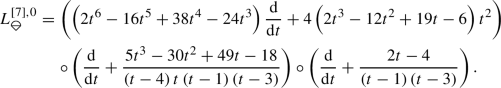
In this section, we give the result for the $\epsilon$-deformed differential equation for the ice-cream cone graph of Fig. 5 generalising the result for $\epsilon =0$ given in [9, 46]. The two-loop (one scoop) ice-cream cone differential form in $D=2-2\epsilon$ dimensions is given by

(117)

with

(118)

We find the following results (some numerical cases are accessible on the SageMath worksheet IceCream-Epsilon.ipynb).

• The equal-kinematics case $\mu _1=\mu _2=m_1=m_2=k_1^2=k_2^2=k_3^2=1$: the differential operator has order 3 and reads

  

  (119)

  with

  

  (120)
  

  (121)
  

  (122)
  

  (123)
  

  (124)

  The $\epsilon ^0$ term factorises as

  

  (125)

  The rightmost operator is the minimal differential equation for the $\epsilon =0$ case [46]

  

  (126)

• The equal-mass case $\mu _1=\mu _2=m_1=m_2=1$ and generic momenta $k_1^2\ne k_2^2\ne k_3^2\ne 1$: the differential operator is of order 3 reads

  

  (127)

  where is of order n. The $\epsilon ^0$ term factorises as

  

  (128)

  where $\mathscr {L}_{a,1}^0$ is a first order operator and the second order differential operator matches the mass specialisation of the differential operator derived algorithmically in Section 5.2 of [46] and using Hodge theory in Section 7.3 of [9]. The highest order coefficient factorises as

  

  (129)

  with

  $$\begin{aligned} c_1(t)= & {} k_{1}^2 k_{2}^2 k_{3}^2 t^2 +t\Big (m_{1}^2 \left( -k_{1}^2 k_{3}^2-k_{2}^2 k_{3}^2+k_{3}^4\right) +m_{2}^2 \left( k_{1}^4-k_{1}^2 k_{2}^2-k_{1}^2 k_{3}^2\right) \nonumber \\{} & {} +(m_{3}+m_{4})^2 \left( -k_{1}^2 k_{2}^2+k_{2}^4-k_{2}^2 k_{3}^2\right) \Big )\nonumber \\{} & {} +m_{1}^4 k_{3}^2+m_{1}^2 m_{2}^2 \left( -k_{1}^2+k_{2}^2-k_{3}^2\right) +m_{1}^2 (m_{3}+m_{4})^2 \left( k_{1}^2-k_{2}^2-k_{3}^2\right) \nonumber \\{} & {} +m_{2}^4 k_{1}^2+m_{2}^2 (m_{3}+m_{4})^2 \left( -k_{1}^2-k_{2}^2+k_{3}^2\right) +k_{2}^2 (m_{3}+m_{4})^4, \end{aligned}$$

  (130)

  and

  $$\begin{aligned} c_2(t)= & {} t^2 k_{1}^2 k_{2}^2 k_{3}^2+t\Big (m_{1}^2 \left( -k_{1}^2 k_{3}^2-k_{2}^2 k_{3}^2+k_{3}^4\right) +m_{2}^2 \left( k_{1}^4-k_{1}^2 k_{2}^2-k_{1}^2 k_{3}^2\right) \nonumber \\{} & {} +(m_{3}-m_{4})^2 \left( -k_{1}^2 k_{2}^2+k_{2}^4-k_{2}^2 k_{3}^2\right) \Big )\nonumber \\{} & {} +m_{1}^4 k_{3}^2+m_{1}^2 m_{2}^2 \left( -k_{1}^2+k_{2}^2-k_{3}^2\right) +m_{1}^2 (m_{3}-m_{4})^2 \left( k_{1}^2-k_{2}^2-k_{3}^2\right) +m_{2}^4 k_{1}^2\nonumber \\{} & {} +m_{2}^2 (m_{3}-m_{4})^2 \left( -k_{1}^2-k_{2}^2+k_{3}^2\right) +k_{2}^2 (m_{3}-m_{4})^4, \end{aligned}$$

  (131)

  and $c^{[41^3]}_3(t,\epsilon )$ a polynomial of degree 5 in t and 1 in $\epsilon$. We recognise the physical thresholds of the ice-cream cone graph given in Section 5.2 of [46] (and given on this page PF-icecream-2loop.ipynb). The $\epsilon$ deformation only affects the position of the apparent singularities.

• The equal-mass case for the scoop $m_1=m_2=1$ and generic masses $\mu _1\ne \mu _2\ne 1$ and generic momenta $k_1^2\ne k_2^2\ne k_3^2\ne 1$: the differential operator has order 3 and has the $\epsilon$ expansion

  

  (132)

  where is of order n. The $\epsilon ^0$ term factorises as

  

  (133)

  where $\mathscr {L}_{a,1}^0$ is a first order operator and the second order differential operator matches the mass specialisation of the differential operator derived algorithmically in Section 5.2 of [46] and using Hodge theory in Section 7.3 of [9]. The leading coefficient factorises as

  

  (134)

  Only the positions of the apparent singularities depend on $\epsilon$. They arise from the roots of the polynomial $c^{[21^5]}_3(t,\epsilon )$ of degree 5 in t and 1 in $\epsilon$.

• Generic masses non-vanishing $m_1\ne m_2\ne \mu _1\ne \mu _2$ and generic momenta $k_1^2\ne k_2^2\ne k_3^2\ne 1$: the differential operator is of order 4 and has the $\epsilon$ expansion

  

  (135)

  The $\epsilon ^0$ term factorises as

  

  (136)

  where $\mathscr {L}_{a,1}^0$ and $\mathscr {L}_{b,1}^0$ are first order operators and the second order differential operator matches the mass specialisation of the differential operator derived algorithmically in Section 5.2 of [46] and using Hodge theory in Section 7.3 of [9]. The leading coefficient factorises as

  

  (137)

  The position of the non-apparent singularities is not affected by the $\epsilon$ deformation, but the apparent depend on $\epsilon$. They arise from the roots of the polynomial $c^{[1^7]}_3(t,\epsilon )$ of degree 11 in t and 2 in $\epsilon$.

Fig. 6

The non-planar triangle-box graph. Dashed lines are massless propagators, and solid lines are massive propagators. The external momenta $k_i$ satisfy $k_1+k_2+k_3=0$ and $k_1^2=k_2^2=0$

5.4 The three-point non-planar triangle-box graph

For the non-planar triangle-box graph in Fig. 6, setting the internal mass to $m=1$ and defining the $2k_1 \cdot k_2 = X$ with $k_1^2=k_2^2=0$ and $k_1+k_2+k_3=0$. We have

(138)

(139)

The integrand of the Feynman integral is the twisted differential form

(140)

an the differential operator is

(141)

5.5 The four-point planar and non-planar double boxes graph

We show how to derive differential equation for the massless box and massless double-box integrals in dimension $D=4-2\epsilon$. Unlike previous cases, these integrals are divergent in four dimensions so the $\epsilon =0$ integrals are not defined.

Fig. 7

The planar massless double-box graphs. The massless external momenta $k_i$ satisfy $k_1+\cdots +k_4=0$ and $k_i^2=0$. The labels of the graph give the index of the edge variable $x_i$

5.5.1 The massless planar double-box graph

The graph polynomials associated with the massless double-box graph in Fig. 7 are given by

$$\begin{aligned} {\textbf {U}}_{\Box \!\Box }&=(x_1+x_2+x_3)(x_4+x_5+x_6)+(x_1+\cdots +x_6)x_7,\nonumber \\ {\textbf {F}}_{\Box \!\Box }(s,t)&=t x_3x_5x_7+s\Big ( (x_1+x_2+x_3) x_4x_6\nonumber \\&\qquad +(x_4+x_5+x_6)x_1x_2+(x_2+x_4)(x_1+x_6)x_7\Big ) \end{aligned}$$

(142)

with the twisted differential in $D=4-2\epsilon$ in the projective space $\mathbb {P}^6$

$$\begin{aligned} \Omega _{\Box \!\Box }^\epsilon (s,t)= {{\textbf {U}}_{\Box \!\Box } \over {\textbf {F}}_{\Box \!\Box }(s,t)^{3}}\left( {\textbf {U}}_{\Box \!\Box }^3\over {\textbf {F}}^2_{\Box \!\Box }(s,t)\right) ^\epsilon \,\Omega _0^{(7)} \, . \end{aligned}$$

(143)

We work with the single scale form $\tilde{\Omega }_{\Box \!\Box }^\epsilon (X)=(-s)^{3+2\epsilon } \Omega _{\Box \!\Box }^\epsilon (s,Xs)$ with the result

$$\begin{aligned} \mathscr {L}_{\Box \!\Box }^\epsilon =(1+X)X^2 \left( \textrm{d}\over \textrm{d}X\right) ^2+(2+3X+\epsilon ) X{\textrm{d}\over \textrm{d}X}+X-\epsilon -2\epsilon ^2. \end{aligned}$$

(144)

Fig. 8

The non-planar massless double-box graphs. The massless external momenta $k_i$ satisfy $k_1+\cdots +k_4=0$ and $k_i^2=0$. The labels of the graph give the index of the edge variable $x_i$

5.5.2 The massless non-planar double-box graph

The graph polynomials associated with the non-planar massless double-box graph in Fig. 8 are given by

(145)

and

(146)

we work with the single scale differential form

(147)

The differential operator we obtain is

(148)

Fig. 9

The Witten ice-cream cone graph in momentum space

5.6 The Witten ice-cream cone diagram

We turn to the Witten ice-cream cone of Fig. 9 in analytic regularisation entering the two-loop correction to the cosmological correlator between conformally coupled field analysed in Section 5.3.4 of [27]. The cosmological correlator is the integration over the energy of the two-loop flat space integral analytically regulated

(149)

where $\vec {k}_1+\vec {k}_2+\vec {k}_3+\vec {k}_4=0$ and $Q=(\omega _3,\vec {k}_3)$ and ${\tilde{Q}}=(\omega _4,-\vec {k}_4)$. The parametric representation is given by the integration over the domain $\Delta _4=\{x_i\ge 0,1\le i\le 4\}$ of the differential form

(150)

with the graph polynomials

(151)

and

(152)

Setting $u= Q^2/(Q-{\tilde{Q}})^2$ and $v={\tilde{Q}}^2/(Q-{\tilde{Q}})^2$ one finds the following Gröbner basis of differential operators³

$$\begin{aligned} \mathscr {L}_1&=\left( 1-u -v\right) v\left( \partial \over \partial v\right) ^{2} -2u v{\partial \over \partial u}{\partial \over \partial v}-(3 \kappa +1)u {\partial \over \partial u}\nonumber \\&\quad +(3 \kappa (1- u-2 v)-v){\partial \over \partial v}-8 \kappa ^2, \end{aligned}$$

(153)

$$\begin{aligned} \mathscr {L}_2&= -u\left( \partial \over \partial u\right) ^{2} +v\left( \partial \over \partial v\right) ^{2} -3 \kappa {\partial \over \partial u}+3 \kappa {\partial \over \partial v}, \end{aligned}$$

(154)

$$\begin{aligned} \mathscr {L}_3&= 2u^2 \left( (u-v)^2+1-2(u+v)\right) \left( \partial \over \partial u\right) ^3\nonumber \\&+v\left( 9 \kappa \left( (u+v-1)^2-2uv\right) -u^2+9 u^2-(v-1)^2-8u(1+v)\right) \left( \partial \over \partial v\right) ^2\nonumber \\&+\left( \kappa ^2\left( -29 u^2+u (43 v+29)-18 (v-1)^2\right) + \kappa \left( 6 u (v+3)-6 (v-1)^2\right) \right. \nonumber \\&\quad \left. +u (5 u-v+1)\right) {\partial \over \partial u}\nonumber \\&+\Big (\kappa ^2 \left( 27 u^2-59 u v-54 u+36 v^2-63 v+27\right) \nonumber \\&\quad -3 \kappa \left( -9 u^2+6 u v+8 u+3 v^2-4 v+1\right) \nonumber \\&-v (u+3 v-3)\Big ){\partial \over \partial v}+24 (\kappa -1) \kappa ^2 (v-u-1)\,. \end{aligned}$$

(155)

6 Three- and higher-loop examples

We now turn to the higher-loop cases of Fig. 10. We first discuss the equal-mass case and then a numerical example at three-loop order with all possible mass configurations.

Fig. 10

Multi-loop sunset

6.1 Minimal differential operator for higher-loop sunset

We now consider the $n-1$-loop sunset integral with $n\ge 4$ in $D=2-2\epsilon$ dimensions. Eq. (9) for this case reads

$$\begin{aligned} I^{\epsilon }_{\circleddash (n-1)}(\vec {m},t,\epsilon )&= \int _{\Delta _n} \Omega ^{\epsilon }_{\circleddash (n-1)}(\vec {m},t,\epsilon ) ; \quad \Omega ^\epsilon _{\circleddash (n-1)}(\vec {m}, t,\epsilon ) ={\Omega ^{(n)}_0\over {\textbf {F}}_{\circleddash (n-1)}(t)}\left( {\textbf {U}}_{\circleddash (n-1)}^n\over {\textbf {F}}_{\circleddash (n-1)}(t)^{n-1}\right) ^\epsilon \end{aligned}$$

(156)

with

$$\begin{aligned} {\textbf { U}}_{\circleddash (n-1)}&= x_1\cdots x_n\sum _{i=1}^n {1\over x_i}\,, \nonumber \\ {\textbf { F}}_{\circleddash (n-1)}(t)&= {\textbf {U}}_{n-1} \sum _{i=1}^n m_i^2x_i-t x_1\cdots x_n \, . \end{aligned}$$

(157)

Notice that ${\textbf {U}}_{\circleddash (n-1)}^n/ {\textbf {F}}_{\circleddash (n-1)}(t)^{n-1}$ is a homogeneous rational function of degree 0 in $(x_1,\ldots ,x_n)$. As usual the differential form is defined in the complement of the vanishing locus of the denominator in $\mathbb {P}^{n-1}\backslash \{{\textbf {F}}_{\circleddash (n-1)}(t)=0\}$. In $D=2$ dimension ($\epsilon =0$) we have a rational differential form $\Omega _{\circleddash (n-1)}^{\epsilon }(\vec {m},t,0)$. The differential operator has been given up to six loops for $\epsilon =0$, and it is in agreement with the Feynman integral being a (relative) period of a Calabi–Yau manifold of complex dimension $n-2$ [11, 12, 14, 17, 18, 20, 80, 87].

6.1.1 The equal-mass case

Already in $D=2$ dimensions, for the sunset integral from three loops on the Griffiths–Dwork algorithm had to be adapted because of the non-isolated singularities of integrand. This was achieved in [46] by using syzygies. The resolution of the linear system in Eq. (29) also takes into account the syzygies when including the $\epsilon$ dependent factor.

For the equal-mass case $m_1=\cdots =m_{l+1}=1$, we find the sunset Feynman integral satisfies the differential equation

$$\begin{aligned} \mathscr {L}_{\circleddash (l)}^\epsilon I_\circleddash (\{1,\ldots ,1\},t,\epsilon )= -(l+1)! {\Gamma (1+\epsilon )^l\over \Gamma (1+l\epsilon )} \end{aligned}$$

(158)

with

$$\begin{aligned} \mathscr {L}_{\circleddash (l)}^{\epsilon } =\sum _{r=0}^{l} \mathscr {L}_{\circleddash (l)}^{r} \epsilon ^r \,, \end{aligned}$$

(159)

where the differential operator is $\mathscr {L}_{\circleddash (l)}^{r}$ is of order $l-r$. In the all equal mass case, the $\epsilon$ dependence takes the particular form $\mathscr {L}_{\circleddash (l)}^{\epsilon } = \mathscr {L}_{\circleddash (l)}^{0}+ O(\epsilon )$ where $\mathscr {L}_{\circleddash (l)}^{0}$ is the differential operator of order l for the all-equal-mass sunset integral in $D=2$ derived in [53] and the $\epsilon$ dependent differential operators have an order $l-r$ where r is the power of $\epsilon$. The order $\epsilon ^0$ differential operator $\mathscr {L}_{\circleddash (l)}^{0}$ reproduces the one derived in [53] up to five-loops using the properties of the Feynman integral in $D=2$ dimensions (see as well [17, 88,89,90,91,92]). By applying the algorithm presented in Sect. 3.1 we derived the differential equations for the all-equal-mass sunset integral up to 20 loop orders. The explicit results are given on the SageMath worksheet Sunset-1mass-Epsilon.ipynb. We notice that the algorithm presented in this work produces the minimal differential operator and does not need any factorisation of the differential operator, contrary to the procedure presented in [90].

6.1.2 The three-loop generic mass cases

For the three-loop sunset with different masses, we find the following results which are given as well on the SageMath worksheet Sunset-Threeloop-Epsilon.ipynb. With the notation of Section 4 of [46]:

• Case [4]: The equal-mass case $m_1=m_2=m_3=m_4$ has already been discussed in the previous section. The $\epsilon ^0$ operator was derived and analysed in [11, 53, 88]. For $\epsilon \ne 0$, the differential operator reads

$$\begin{aligned} \mathscr {L}_{\circleddash (3)}^{[4],\epsilon }= & {} -(t - 16) (t - 4) t^2\left( \textrm{d}\over \textrm{d}t\right) ^3 - 6 (t^3 - 15 t^2 + 32 t) \left( \textrm{d}\over \textrm{d}t\right) ^2 \nonumber \\{} & {} - (7 t^2 - 68 t + 64) \left( \textrm{d}\over \textrm{d}t\right) - t + 4\nonumber \\{} & {} +\epsilon \left( -6 (t - 10 ) t^2 \left( \textrm{d}\over \textrm{d}t\right) ^2 - 6 (3 t - 20 ) t \left( \textrm{d}\over \textrm{d}t\right) +18- 6 t \right) \nonumber \\{} & {} +\epsilon ^2\left( -(11 t^2 - 28 t - 64) \left( \textrm{d}\over \textrm{d}t\right) - 11 t + 14\right) + \epsilon ^3\left( -6 t - 12\right) \,. \end{aligned}$$

(160)

• Case [31]: For two different masses $m_1=m_2=m_3 \ne m_4$ the differential operator is of order 5 and has the following $\epsilon$ dependence

  $$\begin{aligned} \mathscr {L}^{[31],\epsilon }_{\circleddash (3)}= \sum _{r=0}^1 \epsilon ^r \mathscr {L}^{[31],r}_{5}+ \sum _{r=0}^4 \epsilon ^{2+r} \mathscr {L}^{[31],r}_{4-r} \, , \end{aligned}$$

  (161)

  where $\mathscr {L}^{[31],r}_{n}$ are of order n. The order $\epsilon ^0$ operator factorises as

  $$\begin{aligned} \mathscr {L}^{[31],0}_{5}= \mathscr {L}^{[31],0}_{a,1} \circ \mathscr {L}^{[31],\epsilon }_{\circleddash (3)} \, , \end{aligned}$$

  (162)

  where $\mathscr {L}^{[31],0}_{a,1}$ is a first order operator and $\mathscr {L}^{[31],0}_{\circleddash (3)}$ is the fourth order differential operator of the three-loop sunset integral with mass configuration [31] (see in Section 4.3 of [46]). The coefficient of the highest order term $(d/\textrm{d}t)^5$ is given by

  $$\begin{aligned}{} & {} \mathscr {L}^{[31],\epsilon }_{\circleddash (3)}\Big \vert _{(d/\textrm{d}t)^5}= t^3 (t-(m_1-m_4)^2)(t-(m_1+m_4)^2)(t-(3m_1+m_4)^2) \nonumber \\{} & {} \quad \times (t-(3m_1-m_4)^2) q^{[31]}(t,\epsilon ) . \end{aligned}$$

  (163)

  The $\epsilon$ dependence appears only in the apparent singularities determined by the polynomial $q^{[31]}(t,\epsilon )$ of degree 3 in t and 1 in $\epsilon$.

• Case [22]: For two different masses $m_1=m_2\ne m_3 = m_4$ the differential operator has order 6 and the $\epsilon$ expansion

  $$\begin{aligned} \mathscr {L}_{\circleddash (3)}^{[22],\epsilon }= \sum _{r=0}^3 \epsilon ^r \mathscr {L}^{[22],r}_{6}+ \sum _{r=0}^5 \epsilon ^{4+r} \mathscr {L}^{[22],r}_{5-r} \, , \end{aligned}$$

  (164)

  where $\mathscr {L}^{[22],r}_{n}$ are operators of order n. The order $\epsilon ^0$ operator factorises as

  $$\begin{aligned} \mathscr {L}^{[22],0}_{6}= \mathscr {L}^{[22],0}_{a,1} \circ \mathscr {L}^{[22],0}_{b,1} \circ \mathscr {L}^{[22],0}_{\circleddash (3)} \,, \end{aligned}$$

  (165)

  where $\mathscr {L}^{[22],0}_{a,1}$ and $\mathscr {L}^{[22],0}_{b,1}$ are first order operators. $\mathscr {L}^{[22],0}_{\circleddash (3)}$ is the fourth order operator for the three-loop sunset integral with mass configuration [22] given Section 4.3 of [46]. The coefficient of the highest order term $(d/\textrm{d}t)^6$ is given by

  $$\begin{aligned}{} & {} \mathscr {L}^{[22],\epsilon }_{\circleddash (3)}\Big \vert _{(d/\textrm{d}t)^6}= t^4(t-(2m_1)^2)(t-(2m_4)^2)(t-(2m_1+2m_4)^2)\nonumber \\{} & {} \quad \times (t-(2m_1-2m_4)^2) \, q^{[22]}(t,\epsilon ). \end{aligned}$$

  (166)

  The $\epsilon$ dependence appears only in the apparent singularities determined by the polynomial $q^{[22]}(t,\epsilon )$ of degree 4 in t and 3 in $\epsilon$.

• Case [211]: For three different masses $m_1=m_2\ne m_3 \ne m_4$ the differential operator has order 7 and has the $\epsilon$ expansion

  $$\begin{aligned} \mathscr {L}^{[211],\epsilon }_{\circleddash (3)}= \sum _{r=0}^8 \epsilon ^r \mathscr {L}^{[211],r}_{7}+ \sum _{r=0}^6 \epsilon ^{9+r} \mathscr {L}^{[22],r}_{6-r} \,, \end{aligned}$$

  (167)

  where $\mathscr {L}^{[211],r}_{n}$ are operators of order n. The order $\epsilon ^0$ operator factorises as

  $$\begin{aligned} \mathscr {L}^{[211],0}_{7}= \mathscr {L}^{[211],0}_{a,1} \circ \mathscr {L}^{[211],0}_{b,1} \circ \mathscr {L}^{[211],0}_{c,1} \circ \mathscr {L}^{[211],0}_{\circleddash (3)} \,, \end{aligned}$$

  (168)

  where $\mathscr {L}^{[211],0}_{a,1}$, $\mathscr {L}^{[211],0}_{b,1}$ and $\mathscr {L}^{[211],0}_{c,1}$ are first order operators and $\mathscr {L}^{[211],0}_{\circleddash (3)}$ is the fifth order differential operator the three-loop sunset integral with mass configuration [211] given Section 4.3 of [46]. The coefficient of the highest order term $(d/\textrm{d}t)^6$ is given by

  $$\begin{aligned}{} & {} \mathscr {L}^{[211],\epsilon }_{\circleddash (3)}\Big \vert _{(d/\textrm{d}t)^6}= t^5\left( t-(m_{1}-m_{2})^2\right) \left( t-(m_{1}+m_{2})^2\right) \nonumber \\{} & {} \quad \times \left( t-(m_{1}+m_{2}-2 m_{4})^2\right) \left( t-(m_{1}-m_{2}+2 m_{4})^2\right) \left( t-(-m_{1}+m_{2}+2 m_{4})^2\right) \nonumber \\{} & {} \quad \times \left( t-(m_{1}+m_{2}+2 m_{4})^2\right) \, q^{[211]}(t,\epsilon ). \end{aligned}$$

  (169)

  The $\epsilon$ dependence appears only in the apparent singularities determined by the polynomial $q^{[211]}(t,\epsilon )$ of degree 9 in t and 7 in $\epsilon$.

• Case [1111]: For four different masses $m_1\ne m_2\ne m_3 \ne m_4$, the differential operator has order 11 and has the $\epsilon$ expansion

  $$\begin{aligned} \mathscr {L}_{\circleddash (3)}^{[1111],\epsilon }= \sum _{r=0}^{16}\epsilon ^r \mathscr {L}^{[1111],r}_{11}+\sum _{r=0}^{11} \epsilon ^{16+r} \mathscr {L}^{[1111],\epsilon }_{11-r}\, . \end{aligned}$$

  (170)

  The order $\epsilon ^0$ operator factorises as

  $$\begin{aligned} \mathscr {L}^{[1111],0}_{0,11}= \mathscr {L}^{[1111],0}_{a_1,1} \circ \cdots \circ \mathscr {L}^{[1111],0}_{a_5,1} \circ \mathscr {L}^{[1111],0}_{\circleddash (3)}\,, \end{aligned}$$

  (171)

  where $\mathscr {L}^{[1111],\epsilon }_{a_1,1},\ldots , \mathscr {L}^{[1111],\epsilon }_{a_5,1}$ are first order operators and $\mathscr {L}^{[1111],0}_{\circleddash (3)}$ is the sixth order differential operator for the three-loop sunset integral with mass configuration [1111] given in [46]. The coefficient of the highest order term $(\textrm{d}/\textrm{d}t)^{11}$ is given by

  $$\begin{aligned}{} & {} \mathscr {L}^{[1111],\epsilon }_{\circleddash (3)}\Big \vert _{(\textrm{d}/\textrm{d}t)^{11}}= t^{11}\left( t-(m_{1}+m_{2}-m_{3}-m_{4})^2\right) \nonumber \\{} & {} \quad \times \left( t-(m_{1}-m_{2}+m_{3}-m_{4})^2\right) \left( t-(m_{1}+m_{2}+m_{3}-m_{4})^2\right) \nonumber \\{} & {} \quad \times \left( t-(m_{1}-m_{2}-m_{3}+m_{4})^2\right) \left( t-(m_{1}+m_{2}-m_{3}+m_{4})^2\right) \nonumber \\{} & {} \quad \times \left( t-(m_{1}-m_{2}+m_{3}+m_{4})^2\right) \left( t-(-m_{1}+m_{2}+m_{3}+m_{4})^2\right) \nonumber \\{} & {} \quad \times \left( t-(m_{1}+m_{2}+m_{3}+m_{4})^2\right) \, q^{[1111]}(t,\epsilon ). \end{aligned}$$

  (172)

  The $\epsilon$ dependence appears only in the apparent singularities determined by the polynomial $q^{[1111]}(t,\epsilon )$ of degree 17 in t and 16 in $\epsilon$.

7 Summary and discussion

In Sect. 3.1, we have presented an algorithm for deriving inhomogeneous differential equations satisfied by Feynman integrals. At each derivative order the procedure consists of solving the linear systems (29) in order to determine the coefficients $c_{a_1,\ldots ,a_r}({\underline{z}})$ and the inhomogeneous term $\beta _\Gamma$ in (10). Our work introduces an explicit dependence on the regulators $\epsilon$ or $\kappa$, so it is worth discussing their effect on the minimal differential operator and on the singularities of the differential equations.

7.1 Minimal order of the differential operator and number of master integrals

The minimal order differential operator gives direct information about the underlying algebraic-geometry associated with the Feynman integral. The knowledge of this operator is an essential ingredient for identifying if a given Feynman integral is a (relative) period associated with a genus 0, 1 or 2 curve, a Calabi-Yau manifold or other object.

We start by summarising what we have found with the examples studied in this paper:

• For the L-loop sunset integrals, the number of irreducible master integrals is $2^{L+1}-L-2$ [72, 93, 94].

  • The minimal differential operator for the all equal-mass case has order the number of loops L.

  • For generic mass configuration at one-loop we have an operator of order 1, at two-loop an operator of order 4 and at three-loop an operator has order 11.

  • In integer dimensions $\epsilon =0$ the order of the minimal order differential operator for generic kinematics can be less than the number of master integrals. One typical example is the one of the Picard–Fuchs operator $\mathscr {L}_{\circleddash (l)}$ for the multi-loop sunset in $D=2$ dimensions which has for minimal order $2^{L+1}-\left( {\begin{array}{c}L+2\\ \left\lfloor \frac{L+2}{2}\right\rfloor \end{array}}\right)$ for generic mass configurations [46]. The order of the $\epsilon$-dependent differential operator is the same as the number of irreducible master integrals but its $\epsilon$-independent piece $\mathscr {L}_{\circleddash (l)}^0$ is factorisable as $\mathscr {L}_{\circleddash (l)}^0=\mathscr {L}_{1}\circ \mathscr {L}_{\circleddash (l)}$.

• For the two-loop ice-cream cone, the number of irreducible masters is four.

  • In the generic mass and kinematics case, the minimal order of the $\epsilon$-deformed minimal differential operator is four.

  • For special kinematic configurations, the ice-cream cone differential operator is three which is smaller than the number of masters.

We thus see that when $\epsilon \ne 0$ and generic kinematics the order of the differential operator saturates the bound given by the number of irreducible masters. This leads us to formulate the following observation: For general kinematics the minimal (i.e. not factorisable) $\epsilon$-deformed differential operator has the same order as the number of independent master integrals.

7.2 Order reduction

For special kinematics, the minimal order is smaller than the number of master integrals. This reduction of order can be understood by the factorisation of the differential operator

(173)

The reduction of order arises when the integrand has more singularities or more symmetries:

• More singularities: In the case of massless internal lines or massless external kinematics, extra singularities arise thus reducing the genus of the singular locus of the integral. This has for consequence a lowering of the order minimal differential operator.

• More symmetries: Another situation is when special choices of kinematic configurations the integrand of the Feynman integral produce extra symmetries in the space of projective variables ${\underline{x}}$. This leads to new relations between independent (period) integrals, which reduce the number of independent integrals. A typical case is the reduction order of the sunset integral according the mass configurations as given in [11, 17, 18, 46, 90]. These cases are not associated with the appearance of new singularities of the Feynman integral.

In the case of special kinematic configurations that do not lead to new singularities of the integral, the order drop is not detected by either the computation of the Euler characteristic of complement of graph hypersurface in the projective space of the edge variables, nor the computation using the critical points of the Lee–Pomeransky representation [33, 74, 95] nor the Baikov representation [62, 65, 96]. For instance in [97] it was explained how a hidden involution symmetry of the two-loop non-planar double-box allows identifying the hyperelliptic curve of genus 2 when the use of the Baikov representation gave a curve of genus 3. It is shown in [9], using a detailed algebraic-geometrical analysis, that all planar two-loop integrals are either period of rational curves, elliptic curve or genus 2 hyperelliptic curves or minimal order two or four, respectively.

7.3 The regulator dependence

For a differential equation

$$\begin{aligned} c_N(z) {\textrm{d}^Nf(z)\over \textrm{d}z^N}+\cdots + c_0(z) f(z)=0, \end{aligned}$$

(174)

the roots of $c_N(z)$ are the singularities of the differential equation. A root of $c_N(z)$ where the solution f(z) is regular is called an apparent singularity. A root of $c_N(z)$ where the solution has a singularity is a real singularity (See Section 16.4 of [98] for details). For the case of Feynman integrals, the non-apparent singularities of (174) are the roots of the discriminant of the singular locus of the integrand of Feynman integrals [9].

We have noticed that the dimensional regulator $\epsilon$ appears only in the apparent singularities of the differential operator $\mathscr {L}_\Gamma ^\epsilon$. This means that the $\epsilon$ deformation does not change the position of the real singularities, but it affects the local behaviour (the monodromy) of the solution near the singularity. The physical interpretation of this is that the kinematic singularities (the position of the thresholds and pseudo-thresholds) of a Feynman integral are independent of the space-time dimension. However, the local behaviour of the integral near the thresholds and pseudo-thresholds does change with the space-time dimension. The latter has been used with great success when decomposing amplitudes using the generalised unitarity method [99].

7.4 Outlook

We have presented a generalisation of the Griffiths–Dwork reduction for deriving the differential operator acting on Feynman integrals in dimensional regularisation or analytic regularisation. The algorithm makes a special use of the fact that the twist from the regularisation is the power of a degree zero homogeneous rational function in the edge variables. The procedure amounts to solving linear systems which is done using FiniteFlow routines [51].

We have applied the algorithm to various cases and derived the inhomogeneous partial differential equations satisfied by the integrand of the Feynman integral in parametric representation. In dimensional regularisation we have confirmed that the order the differential operators is smaller or equal to the number of master integrals. The order of the differential operators is lower for the cases of the kinematic invariants where the integrand presents more symmetry (equal-masses, special kinematics,...) or more singularities (massless internal or external states). Something that was already noticed in the case of finite integrals [46] but stays true for the regulated integrals.

One motivation for presenting this algorithm is its application to Feynman integrals in analytical regularisation which arise in the evaluation of the cosmological correlators [25, 27, 100], since the commonly used integration-by-part algorithms need to be adapted to the case of analytic regularisation with several propagators with generalised powers.

We have shown as well how to derive a Gröbner basis of partial differential operators in some multiple scale cases. The differential operators produced by the algorithm of this paper might arise as specialisation of the system of partial differential operators obtained by GKZ approach. The restriction of the GKZ D-module is a difficult open problem, which we leave for further investigations.

The Bessel representation for the sunset graphs

Following the steps in Section 8 of [53] gives the following Bessel integral representation for the multi-loop sunset integrals in $D=2-2\epsilon$ dimensions

$$\begin{aligned}{} & {} I_{\circleddash (n-1)}^\epsilon (\vec {m},t,\epsilon )= {2^{(n-1) (1-\epsilon )} t^{\epsilon \over 2} \over (m_1\cdots m_{L+1})^{\epsilon } \Gamma (1+(n-1)\epsilon )}\nonumber \\{} & {} \quad \times \int _0^\infty I_{-\epsilon }(\sqrt{t} x) \prod _{i=1}^{n}K_{-\epsilon }(m_ix)\, x^{1+\epsilon (n-1)}\textrm{d}x. \end{aligned}$$

(175)

This integral representation is valid for $t<(m_1+\cdots +m_{n})^2$. For $x\rightarrow 0$ we have

$$\begin{aligned} \lim _{x\rightarrow 0} I_{-\epsilon }(x)\simeq \left( x\over 2\right) ^{\epsilon }; \qquad \lim _{x\rightarrow 0} K_{-\epsilon }(x) \simeq \left( x\over 2\right) ^{\epsilon } \end{aligned}$$

(176)

and the integral converges as long as $2+(n-1)\epsilon >0$ which is the condition $D=2-2\epsilon < 2n/(n-1)$ for the absence of ultraviolet divergences for the $n-1$-loop massive sunset.

Using this representation and applying the creative telescoping algorithm [47,48,49,50], we have checked the results obtained the extended Griffiths–Dwork reduction. The creative telescoping algorithm builds an annihilator

$$\begin{aligned} \mathscr {T}(t,\partial _t; x,\partial _x)= \mathscr {L}(t,\partial _t)+ \mathscr {C}( t,\partial _t; x,\partial _x) \end{aligned}$$

(177)

of the integrand $f(t,x):= I_{-\epsilon }(\sqrt{t} x) \prod _{i=1}^{L+1}K_{-\epsilon }(m_ix)\, x^{1+\epsilon (n-1)}$ such that

$$\begin{aligned} \mathscr {T}(t,\partial _t; x,\partial _x) f(t,x)=\mathscr {L}(t,\partial _t)i(t,x)+ \mathscr {C}( t,\partial _t; x,\partial _x) f(t,x)=0 \end{aligned}$$

(178)

implying that $\mathscr {L}(t,\partial _t)f(t,x)$ is the operator acting on the integral because the domain of integration is independent of t. On an ordinary laptop, the results for the equal-mass case and up to twenty loops order are obtained in a few second to a few minutes, which is of the same order of time as the generalised Griffiths–Dwork reduction presented in the main text of this work.

References

Golubeva, V.A.: Some problems in the analytic theory of Feynman integrals. Russ. Math. Surv. 31, 139 (1976)
Pham, F.: Introduction à l’étude topologique des singularités de Landau. Gauthier-Villars, Paris (1967)
Panzer, E.: Feynman Integrals and Hyperlogarithms. PhD Humboldt U Thesis (2015). [arXiv:1506.07243 [math-ph]]
Duhr, C.: Function theory for multiloop Feynman integrals. Ann. Rev. Nucl. Part. Sci. 69, 15–39 (2019)
Mizera, S.: “Status of Intersection Theory and Feynman Integrals,” PoS MA2019, 016 (2019) [arXiv:2002.10476 [hep-th]]
Travaglini, G., Brandhuber, A., Dorey, P., McLoughlin, T., Abreu, S., Bern, Z., Bjerrum-Bohr, N.E.J., Blümlein, J., Britto, R., Carrasco, J.J.M., et al.: The SAGEX review on scattering amplitudes. J. Phys. A 55(44), 443001 (2022). [arXiv:2203.13011 [hep-th]]
Weinzierl, Stefan: Quantum field theory. In Feynman Integrals: A Comprehensive Treatment for Students and Researchers, pages 101–133. Springer, (2022). [arXiv:2201.03593]
Badger, S., Henn, J., Plefka, J.C., Zoia, S.: “Scattering Amplitudes in Quantum Field Theory,” Lecture Notes Physics. 1021, pp. (2024) [arXiv:2306.05976 [hep-th]]
Doran, C.F., Harder, A., Pichon-Pharabod, E., Vanhove, P.: “Motivic Geometry of Two-Loop Feynman Integrals,” [arXiv:2302.14840 [math.AG]]
Brown, Francis: On the periods of some Feynman integrals. 10 (2009). [arXiv:0910.0114]
Bloch, Spencer, Kerr, Matt, Vanhove, Pierre: A Feynman integral via higher normal functions. Compos. Math. 151(12), 2329–2375 (2015). [arXiv:1406.2664]
Bloch, Spencer, Kerr, Matt, Vanhove, Pierre: Local mirror symmetry and the sunset Feynman integral. Adv. Theor. Math. Phys. 21, 1373–1453 (2017). [arXiv:1601.08181]
Bourjaily, J.L., He, Y.H., Mcleod, A.J., Von Hippel, M., Wilhelm, M.: Traintracks through Calabi–Yau manifolds: scattering amplitudes beyond elliptic polylogarithms. Phys. Rev. Lett. 121(7), 071603 (2018). [arXiv:1805.09326 [hep-th]]
Bourjaily, J.L., McLeod, A.J., Vergu, C., Volk, M., Von Hippel, M., Wilhelm, M.: Embedding feynman integral (Calabi–Yau) geometries in weighted projective space. JHEP 01, 078 (2020). [arXiv:1910.01534 [hep-th]]
Bourjaily, J.L., McLeod, A.J., von Hippel, M., Wilhelm, M.: Bounded collection of feynman integral Calabi–Yau geometries. Phys. Rev. Lett. 122(3), 031601 (2019). [arXiv:1810.07689 [hep-th]]
Klemm, A., Nega, C., Safari, R.: The \(l\)-loop banana amplitude from Gkz systems and relative Calabi–Yau periods. JHEP 04, 088 (2020). [arXiv:1912.06201 [hep-th]]
Bönisch, K., Fischbach, F., Klemm, A., Nega, C., Safari, R.: Analytic structure of all loop banana integrals. JHEP 05, 066 (2021). [arXiv:2008.10574 [hep-th]]
Bönisch, K., Duhr, C., Fischbach, F., Klemm, A., Nega, C.: Feynman integrals in dimensional regularization and extensions of Calabi–Yau motives. JHEP 09, 156 (2022). [arXiv:2108.05310 [hep-th]]
Bourjaily, J.L., Broedel, J., Chaubey, E., Duhr, C., Frellesvig, H., Hidding, M., Marzucca, R., McLeod, A.J., Spradlin, M., Tancredi, L., et al.: “Functions Beyond Multiple Polylogarithms for Precision Collider Physics,” [arXiv:2203.07088 [hep-ph]]
Forum, A., von Hippel, M.: A symbol and coaction for higher-loop sunrise integrals. SciPost Phys. Core 6, 050 (2023). [arXiv:2209.03922 [hep-th]]
Duhr, C., Klemm, A., Loebbert, F., Nega, C., Porkert, F.: Yangian–Invariant fishnet integrals in two dimensions as volumes of Calabi–Yau varieties. Phys. Rev. Lett. 130(4), 4 (2023). [arXiv:2209.05291 [hep-th]]
Frellesvig, H., Morales, R., Wilhelm, M.: “Calabi-Yau meets Gravity: A Calabi-Yau three-fold at fifth post-Minkowskian order,” [arXiv:2312.11371 [hep-th]]
Pögel, S., Wang, X., Weinzierl, S.: “Feynman Integrals, Geometries and Differential Equations,” PoS RADCOR2023, 007 (2024) [arXiv:2309.07531 [hep-th]]
Klemm, A., Nega, C., Sauer, B., Plefka, J.: “Cy in the Sky,” [arXiv:2401.07899 [hep-th]]
Heckelbacher, T., Sachs, I., Skvortsov, E., Vanhove, P.: Analytical evaluation of cosmological correlation functions. JHEP 08, 139 (2022). [arXiv:2204.07217 [hep-th]]
Heckelbacher, T., Sachs, I., Skvortsov, E., Vanhove, P.: Analytical evaluation of \(\text{ AdS}_{4}\) witten diagrams as flat space multi-loop Feynman integrals. JHEP 08, 052 (2022). [arXiv:2201.09626 [hep-th]]
Chowdhury, C., Lipstein, A., Mei, J., Sachs, I., Vanhove, P.: “The Subtle Simplicity of Cosmological Correlators,” [arXiv:2312.13803 [hep-th]]
Vanhove, P.: “Feynman Integrals, Toric Geometry and Mirror Symmetry,” [arXiv:1807.11466 [hep-th]]
de la Cruz, L.: Feynman integrals as a-hypergeometric functions. JHEP 12, 123 (2019). [arXiv:1907.00507 [math-ph]]
Klausen, R.P.: Hypergeometric series representations of Feynman integrals by Gkz hypergeometric systems. JHEP 04, 121 (2020). [arXiv:1910.08651 [hep-th]]
Feng, T.F., Chang, C.H., Chen, J.B., Zhang, H.B.: Gkz-hypergeometric systems for Feynman integrals. Nucl. Phys. B 953, 114952 (2020). [arXiv:1912.01726 [hep-th]]
Ananthanarayan, B., Banik, S., Bera, S., Datta, S.: Feyngkz: a mathematica package for solving Feynman integrals using Gkz hypergeometric systems. Comput. Phys. Commun. 287, 108699 (2023). [arXiv:2211.01285 [hep-th]]
Agostini, D., Fevola, C., Sattelberger, A.L., Telen, S.: “Vector Spaces of Generalized Euler Integrals,” [arXiv:2208.08967 [math.AG]]
Matsubara-Heo, S.J., Mizera, S., Telen, S.: Four lectures on Euler integrals. SciPost Phys. Lect. Notes 75, 1 (2023). [arXiv:2306.13578 [math-ph]]
Munch, H.J.: “Feynman Integral Relations from Gkz Hypergeometric Systems,” PoS LL2022, 042 (2022) [arXiv:2207.09780 [hep-th]]
Klausen, R.P.: Kinematic singularities of Feynman integrals and principal A-determinants. JHEP 02, 004 (2022). [arXiv:2109.07584 [hep-th]]
Chestnov, V., Matsubara-Heo, S.J., Munch, H.J., Takayama, N.: Restrictions of Pfaffian systems for Feynman integrals. JHEP 11, 202 (2023). [arXiv:2305.01585 [hep-th]]
Dlapa, C., Helmer, M., Papathanasiou, G., Tellander, F.: Symbol alphabets from the Landau singular locus. JHEP 10, 161 (2023). [arXiv:2304.02629 [hep-th]]
Griffiths, P.A.: On the periods of certain rational integrals. Ann. Math. 90, 460–541 (1969)
Griffiths, P.A.: The Residue Calculus and Some Transcendental Results in Algebraic Geometry, I. Presented at the (1966)
Griffiths, P.A.: The residue calculus and some transcendental results in algebraic geometry, II. Proc. National Acad. Sci. 55, 1392–1395 (1966)
Dwork, B.: On the zeta function of a hypersurface. Inst. Hautes Études Sci. Publ. Math. 12, 5–68 (1962)
Dwork, B.: On the zeta function of a hypersurface: II. Ann. Math. 80, 227–299 (1964)
Müller-Stach, S., Weinzierl, S., Zayadeh, R.: A second-order differential equation for the two-loop sunrise graph with arbitrary masses. Commun. Num. Theor. Phys. 6, 203–222 (2012). [arXiv:1112.4360 [hep-ph]]
Müller-Stach, Stefan, Weinzierl, Stefan, Zayadeh, Raphael: Picard-Fuchs equations for Feynman integrals. Commun. Math. Phys. 326(1), 237–249 (2014). [arXiv:1212.4389]
Lairez, P., Vanhove, P.: Algorithms for minimal Picard–Fuchs operators of Feynman integrals. Lett. Math. Phys. 113(2), 37 (2023). [arXiv:2209.10962 [hep-th]]
Chyzak, Frédéric.: extension of Zeilberger’s fast algorithm to general holonomic functions. Discrete Math. 217(1–3), 115–134 (2000)
Chyzak, Frédéric.: “Creative Telescoping for Parametrised Integration and Summation”, Les cours du CIRM, 2(1). Course no II, 1–37 (2011)
Bostan, A., Lairez, P., Salvy, B.: ”Creative telescoping for rational functions using the Griffiths–Dwork method.” In Proceedings of the 38th International Symposium on Symbolic and Algebraic Computation (pp. 93–100)
Koutschan, C.: “HolonomicFunctions (user’s guide).” Technical Report 10-01, RISC Report Series, Johannes Kepler University, Linz, Austria, 2010. http://www.risc.jku.at/research/combinat/software/HolonomicFunctions/
Peraro, T.: Finiteflow: multivariate functional reconstruction using finite fields and dataflow graphs. JHEP 07, 031 (2019). [arXiv:1905.08019 [hep-ph]]
Nakanishi, Noboru: Graph Theory and Feynman Integrals, vol. 11. Routledge, London (1971)
Vanhove, P.: The physics and the mixed Hodge structure of Feynman integrals. Proc. Symp. Pure Math. 88, 161–194 (2014). [arXiv:1401.6438 [hep-th]]
Bogner, C., Weinzierl, S.: Feynman graph polynomials. Int. J. Mod. Phys. A 25, 2585–2618 (2010). [arXiv:1002.3458 [hep-ph]]
Bloch, Spencer, Esnault, Hélène., Kreimer, Dirk: On motives associated to graph polynomials. Commun. Math. Phys. 267(1), 181–225 (2006). [arXiv:math/0510011]
Speer, E.R.: “Generalized Feynman Amplitudes,” vol. 62 of Annals of Mathematics Studies. Princeton University Press, New Jersey, (1969)
Aomoto, K.: Les équations aux différences linéaires et les intégrales des fonctions multiformes. J. Fac. Sci. Univ. Tokyo 22(3), 271–297 (1975)
Aomoto, K.: On vanishing of cohomology attached to certain many valued meromorphic functions. J. Math. Soc. Japan 27(2), 248–255 (1975)
Aomoto, K.: Configurations and invariant Gauss–Manin connections of integrals I. Tokyo J. Math. 5, 249–287 (1982)
Aomoto, K., Kita, M.: Theory of Hypergeometric Functions. Springer Monographs in Mathematics, Springer-Verlag, Tokyo (2011)
Mizera, S.: Scattering amplitudes from intersection theory. Phys. Rev. Lett. 120(14), 141602 (2018). [arXiv:1711.00469 [hep-th]]
Frellesvig, H., Gasparotto, F., Mandal, M.K., Mastrolia, P., Mattiazzi, L., Mizera, S.: Vector space of Feynman integrals and multivariate intersection numbers. Phys. Rev. Lett. 123(20), 201602 (2019). [arXiv:1907.02000 [hep-th]]
Caron-Huot, S., Pokraka, A.: Duals of Feynman integrals. Part I. Differential equations. JHEP 12, 045 (2021). [arXiv:2104.06898 [hep-th]]
Caron-Huot, S., Pokraka, A.: Duals of Feynman integrals. Part II. generalized unitarity. JHEP 04, 078 (2022). [arXiv:2112.00055 [hep-th]]
Cacciatori, S.L., Conti, M., Trevisan, S.: Co-homology of differential forms and Feynman diagrams. Universe 7(9), 328 (2021). [arXiv:2107.14721 [hep-th]]
Fontana, G., Peraro, T.: Reduction to master integrals via intersection numbers and polynomial expansions. JHEP 08, 175 (2023). [arXiv:2304.14336 [hep-ph]]
Munch, H.J.: “Evaluating Feynman Integrals Using D-modules and Tropical Geometry,” [arXiv:2401.00891 [hep-th]]
Brunello, G., Chestnov, V., Crisanti, G., Frellesvig, H., Mandal, M.K., Mastrolia, P.: “Intersection Numbers, Polynomial Division and Relative Cohomology,” [arXiv:2401.01897 [hep-th]]
De, S., Pokraka, A.: “Cosmology Meets Cohomology,” [arXiv:2308.03753 [hep-th]]
Teschke, T.: “General Relativity from Intersection Theory and Loop Integrals,” [arXiv:2401.01920 [hep-th]]
Kashiwara, M., Kawai, T.: Holonomic systems of linear differential equations and Feynman integrals. Publ. Res. Inst. Math. Sci. Kyoto 12, 131 (1977)
T. Bitoun, C. Bogner, R. P. Klausen and E. Panzer, “Feynman Integral Relations from Parametric Annihilators,” Lett. Math. Phys. 109(3), 497-564 (2019) [arXiv:1712.09215 [hep-th]]
Smirnov, A.V., Petukhov, A.V.: The number of master integrals is finite. Lett. Math. Phys. 97, 37–44 (2011). [arXiv:1004.4199 [hep-th]]
Lee, R.N., Pomeransky, A.A.: Critical points and number of master integrals. JHEP 11, 165 (2013). [arXiv:1308.6676 [hep-ph]]
Mastrolia, P., Mizera, S.: Feynman integrals and intersection theory. JHEP 02, 139 (2019). [arXiv:1810.03818 [hep-th]]
van der Put, M., Singer, M.F.: Galois Theory of Linear Differential Equations, Vol. 328. Springer: 2003. An electronic version of this book is available at http://www4.ncsu.edu/~singer/ms_papers.html
van Hoeij, M.: Factorization of differential operators with rational functions coefficients. J. Symb. Comput. 24, 537–561 (1997)
Chyzak, Frédéric, Goyer, Alexandre, Mezzarobba, Marc: Symbolic-numeric factorization of differential operators. In: Proceedings of the 2022 International Symposium on Symbolic and Algebraic Computation, ISSAC ’22, page 73-82, New York, NY, USA, (2022). Association for Computing Machinery. [arXiv:2205.08991]
Goyer, Alexandre: A Sage package for the symbolic-numeric factorization of linear differential operators. ACM Commun. Computer Algebra 55(2), 44–48 (2021)
Bloch, S., Vanhove, P.: The elliptic dilogarithm for the sunset graph. J. Number Theor. 148, 328–364 (2015). [arXiv:1309.5865 [hep-th]]
Caffo, M., Czyz, H., Laporta, S., Remiddi, E.: The master differential equations for the two loop sunrise Selfmass amplitudes. Nuovo Cim. A 111, 365–389 (1998). [arXiv:hep-th/9805118 [hep-th]]
Remiddi, E., Tancredi, L.: Schouten identities for Feynman graph amplitudes; the master integrals for the two-loop massive sunrise graph. Nucl. Phys. B 880, 343–377 (2014). [arXiv:1311.3342 [hep-ph]]
Adams, L., Bogner, C., Weinzierl, S.: The two-loop sunrise graph with arbitrary masses. J. Math. Phys. 54, 052303 (2013). [arXiv:1302.7004 [hep-ph]]
Remiddi, E., Tancredi, L.: Differential equations and dispersion relations for Feynman amplitudes. The two-loop massive sunrise and the kite integral. Nucl. Phys. B 907, 400–444 (2016). [arXiv:1602.01481 [hep-ph]]
Broadhurst, D.J.: The master two loop diagram with masses. Z. Phys. C 47, 115–124 (1990)
Adams, L., Bogner, C., Schweitzer, A., Weinzierl, S.: The kite integral to all orders in terms of elliptic polylogarithms. J. Math. Phys. 57(12), 122302 (2016). [arXiv:1607.01571 [hep-ph]]
Candelas, P., de la Ossa, X., Kuusela, P., McGovern, J.: Mirror symmetry for five-parameter Hulek–Verrill manifolds. SciPost Phys. 15(4), 144 (2023). [arXiv:2111.02440 [hep-th]]
Pögel, S., Wang, X., Weinzierl, S.: The three-loop equal-mass banana integral in \({\varepsilon }\)-factorised form with meromorphic modular forms. JHEP 09, 062 (2022). [arXiv:2207.12893 [hep-th]]
Pögel, S., Wang, X., Weinzierl, S.: Taming Calabi–Yau Feynman integrals: the four-loop equal-mass banana integral. Phys. Rev. Lett. 130(10), 101601 (2023). [arXiv:2211.04292 [hep-th]]
Pögel, S., Wang, X., Weinzierl, S.: Bananas of equal mass: any loop, any order in the dimensional regularisation parameter. JHEP 04, 117 (2023). [arXiv:2212.08908 [hep-th]]
Mishnyakov, V., Morozov, A., Suprun, P.: Position space equations for banana Feynman diagrams. Nucl. Phys. B 992, 116245 (2023). [arXiv:2303.08851 [hep-th]]
Mishnyakov, V., Morozov, A., Reva, M.: “On Factorization Hierarchy of Equations for Banana Feynman Amplitudes,” [arXiv:2311.13524 [hep-th]]
Kalmykov, M.Y., Kniehl, B.A.: Mellin–Barnes representations of feynman diagrams, linear systems of differential equations, and polynomial solutions. Phys. Lett. B 714, 103–109 (2012). [arXiv:1205.1697 [hep-th]]
Kalmykov, M.Y., Kniehl, B.A.: Counting the number of master integrals for sunrise diagrams via the Mellin–Barnes representation. JHEP 07, 031 (2017). https://doi.org/10.1007/JHEP07(2017)031. [arXiv:1612.06637 [hep-th]]
Fevola, C., Mizera, S., Telen, S.: “Landau Singularities Revisited,” [arXiv:2311.14669 [hep-th]]
Frellesvig, H., Papadopoulos, C.G.: Cuts of Feynman integrals in Baikov representation. JHEP 1704, 083 (2017). [arXiv:1701.07356 [hep-ph]]
Marzucca, R., McLeod, A.J., Page, B., Pögel, S., Weinzierl, S.: “Genus Drop in Hyperelliptic Feynman Integrals,” [arXiv:2307.11497 [hep-th]]
Ince, E.L.: Ordinary Differential Equations. Courier Corporation, Chennai (1956)
Bern, Z., Huang, Yt.: Basics of generalized unitarity. J. Phys. A 44, 454003 (2011). [arXiv:1103.1869 [hep-th]]
Chowdhury, C., Singh, K.: Analytic results for loop-level momentum space witten diagrams. JHEP 12, 109 (2023). [arXiv:2305.18529 [hep-th]]
Acknowledgements
We would like to thank Pierre Lairez, Eric Pichon-Pharabod for discussions. We also thank Tiziano Peraro for correspondence on the use of FiniteFlow. P.V. thanks the LAPTh for hospitality when this work has been completed. The work of P.V. has received funding from the ANR grant “SMAGP” ANR-20-CE40-0026-01. P.V. acknowledges support of the Institut Henri Poincaré (UAR 839 CNRS-Sorbonne Université), and LabEx CARMIN (ANR-10-LABX-59-01). The work of LDLC is supported by the European Research Council under grant ERC-AdG-885414.
Author information
Authors and Affiliations
Corresponding author
Ethics declarations
Conflict of interest statement
On behalf of all authors, the corresponding author states that there is no conflict of interest.
Additional information
Publisher's Note
Springer Nature remains neutral with regard to jurisdictional claims in published maps and institutional affiliations.