Global Solutions and Time Decay of the Non-cutoff Vlasov–Maxwell–Boltzmann System in the Whole Space

Abstract

The global in time classical solutions to the Cauchy problem of the Vlasov–Maxwell–Boltzmann system near Maxwellians are obtained under the lower regularity index assumption and the weaker smallness condition on the initial perturbation in comparison with the work (Duan et al. in Kinet Relat Models 6(1):159–204, 2013). In particular, we show the relation between time decay rates and spatial derivatives of solutions.Our analysis relies on a refined energy estimates and the interpolation techniques between negative Sobolev norms and positive Sobolev norms without linear decay analysis.

1 Introduction and Main Results

This paper concerns the existence and time decay rates of global in time classical solutions to the Cauchy problem of the Vlasov–Maxwell–Boltzmann system (called VMB for simplicity) near Maxwellians, which takes the form:

$$\begin{aligned} {\left\{ \begin{array}{ll} \partial _tF_++ v \cdot \nabla _xF_++(E+v\times B)\cdot \nabla _{ v }F_+=Q(F_+,F_+)+Q(F_+,F_-),\\ \partial _tF_-+ v \cdot \nabla _xF_--(E+v\times B)\cdot \nabla _{ v }F_-=Q(F_-,F_+)+Q(F_-,F_-),\\ \partial _tE-\nabla _x\times B=-\int _{\mathbb {R}^3}v(F_+-F_-)dv,\\ \partial _tB+\nabla _x\times E=0,\\ \nabla _x\cdot E=\int _{\mathbb {R}^3}(F_+-F_-)dv,\quad \nabla _x\cdot B=0. \end{array}\right. } \end{aligned}$$

(1.1)

with prescribed initial data

$$\begin{aligned} F_\pm (0,x,v)=F_{0,\pm }(v,x), \quad E(0,x)=E_0(x), \quad B(0,x)=B_0(x) \end{aligned}$$

(1.2)

which satisfy the compatibility conditions

$$\begin{aligned} \nabla _x\cdot E_0=\int _{\mathbb {R}^3}(F_{0,+}-F_{0,-})dv, \quad \nabla _x\cdot B_0=0. \end{aligned}$$

Here the unknown functions $F_\pm = F_\pm (t,x, v) \ge 0$ are the number density functions for the ions ($+$) and electrons ($-$) with position $x = (x_1, x_2, x_3)\in {\mathbb {R}}^3$, velocity $v=( v_1, v_2, v_3) \in {\mathbb {R}}^3$ at time $t\ge 0$, respectively. E(t, x) and B(t, x) denote the electro and magnetic fields, respectively. The Boltzmann collision operator Q is given by

$$\begin{aligned} Q(F,G)(v) =\int _{\mathbb {R}^3\times \mathbb {S}^2}{\mathbf B}(v-u,\sigma )\{F(v')G(u')-F(v)G(u)\} d\sigma du \end{aligned}$$

where in terms of velocities u and v before the collision, velocities $v'$ and $u'$ after the collision are defined by

$$\begin{aligned} v'=\frac{v+u}{2}+\frac{|v-u|}{2}\sigma ,\ \ \ \ u'=\frac{v+u}{2}-\frac{|v-u|}{2}\sigma . \end{aligned}$$

The Boltzmann collision kernel ${\mathbf B}(v-u,\sigma )$ depends only on the relative velocity $|v-u|$ and on the deviation angle $\theta$ given by $\cos \theta =\langle \sigma ,\ (v-u)/{|v-u|}\rangle$, where $\langle \cdot , \cdot \rangle$ is the usual dot product in $\mathbb {R}^3$. As in [1–3, 7], we suppose that ${\mathbf B}(v-u,\sigma )$ is supported on $\cos \theta \ge 0$. Notice also that all the physical parameters have been chosen to be unit for simplicity of presentation.

Throughout the paper, the collision kernel is further supposed to satisfy the following assumptions:

• (A1). ${\mathbf B}(v-u,\sigma )$ takes the product form in its argument as

  $$\begin{aligned} {\mathbf B}(v-u,\sigma )=\Phi (|v-u|){\mathbf b}(\cos \theta ) \end{aligned}$$

  with $\Phi$ and ${\mathbf b}$ being non-negative functions;

• (A2). The angular function $\sigma \rightarrow {\mathbf b}(\langle \sigma ,(v-u)/|v-u|\rangle )$ is not integrable on ${\mathbb {S}}^2$, i.e.

  $$\begin{aligned} \int _{{\mathbb {S}}^2}{\mathbf b}(\cos \theta )d\sigma =2\pi \int _0^{\pi /2}\sin \theta {\mathbf b}(\cos \theta )d\theta =\infty . \end{aligned}$$

  Moreover, there are two positive constants $c_b>0, 0<s<1$ such that

  $$\begin{aligned} \frac{c_b}{\theta ^{1+2s}}\le \sin \theta {\mathbf b}(\cos \theta )\le \frac{1}{c_b\theta ^{1+2s}}; \end{aligned}$$

• (A3). The kinetic function $z\rightarrow \Phi (|z|)$ satisfies

  $$\begin{aligned} \Phi (|z|)=C_\Phi |z|^\gamma \end{aligned}$$

  for some positive constant $C_\Phi > 0.$ Here we should notice that the exponent $\gamma >-3$ is determined by the intermolecular interactive mechanism.

It is convenient to call hard potentials when $\gamma +2s\ge 0$ and soft potentials when $-3<\gamma <-2s$ with $0<s<1$. Interested readers may refer to the textbooks [12, 14, 20] for more details. The current work is restricted to the case of

$$\begin{aligned} \max \left\{ -3,-\frac{3}{2}-2s\right\} <\gamma <-2s, \ \ \frac{1}{2}\le s<1. \end{aligned}$$

(1.3)

Our goal of the paper is to study the Cauchy problem (1.1) around the following normalized global Maxwellian $\mu =\mu (v)=(2\pi )^{-{3}/{2}}e^{-| v |^2/2}.$ For this purpose, we define the perturbation $f_\pm =f_\pm (t,x, v)$ by $F_\pm (t, x, v ) = \mu + \mu ^{1/2}f_\pm (t, x, v).$ Then, the VMB system (1.1) is reformulated as

$$\begin{aligned} {\left\{ \begin{array}{ll} \partial _tf_\pm + v \cdot \nabla _xf_\pm \pm (E+v\times B)\cdot \nabla _{ v }f_\pm \mp E \cdot v \mu ^{1/2}\mp \frac{1}{2} E\cdot v f_\pm +{ L}_\pm f={\Gamma }_\pm (f,f),\\ \partial _tE-\nabla _x\times B=-\int _{\mathbb {R}^3}v\mu ^{1/2}(f_+-f_-)dv,\\ \partial _tB+\nabla _x\times E=0,\\ \nabla _x\cdot E=\int _{\mathbb {R}^3}\mu ^{1/2}(f_+-f_-)dv,\quad \nabla _x\cdot B=0, \end{array}\right. } \end{aligned}$$

(1.4)

with initial data

$$\begin{aligned} f_\pm (0,x,v)=f_{0,\pm }(x,v), \quad E(0,x)=E_0(x), \quad B(0,x)=B_0(x), \end{aligned}$$

(1.5)

which satisfy the compatibility conditions

$$\begin{aligned} \nabla _x\cdot E_0=\int _{\mathbb {R}^3}\mu ^{1/2}(f_{0,+}-f_{0,-})dv, \quad \nabla _x\cdot B_0=0. \end{aligned}$$

(1.6)

If we denote $f=\left[ f_+,f_-\right]$, then (1.4)_1 can be written as

$$\begin{aligned} \partial _t f+v\cdot \nabla _xf+q_0(E+v\times B)\cdot \nabla _v f-E\cdot v\mu ^{1/2}q_1+Lf=\frac{q_0}{2}E\cdot vf+\Gamma (f,f) \end{aligned}$$

(1.7)

where $q_0=diag(1,-1)$, $q_1=[1,-1]$, the linearized collision operator L and the nonlinear collision term $\Gamma (f,f)$ are respectively defined by

$$\begin{aligned} Lf=[L_+f,L_-f],\quad \quad \quad \Gamma (f,g)=[\Gamma _+(f,g),\Gamma _-(f,g)] \end{aligned}$$

with

$$\begin{aligned} \begin{aligned} { L}_\pm f =&-{\varvec{\mu }}^{-1/2} \big \{{Q( \mu ,{\varvec{\mu }}^{1/2}(f_\pm +f_\mp ))+ 2Q( \mu ^{1/2}f_\pm , \mu )}\big \},\\ { \Gamma }_{\pm }(f,g) =&{\varvec{\mu }}^{-1/2}Q\big ({\varvec{\mu }}^{1/2}f_{\pm },{\varvec{\mu }}^{1/2}g_\pm \big )+{\varvec{\mu }}^{-1/2}Q\big ({\varvec{\mu }}^{1/2}f_{\pm },{\varvec{\mu }}^{1/2}g_\mp \big ). \end{aligned} \end{aligned}$$

For the linearized Boltzmann collision operator L, it is well known [9] that it is non-negative and the null space of L is given by

$$\begin{aligned} {\mathcal { N}}={\text {span}}\left\{ [1,0]\mu ^{1/2} , [0,1]\mu ^{1/2}, [v_i,v_i]{\mu }^{1/2} (1\le i\le 3),[|v|^2,|v|^2]{\varvec{\mu }}^{1/2}\right\} . \end{aligned}$$

If we define ${\mathbf P}$ as the orthogonal projection from $L^2({\mathbb {R}}^3_ v)\times L^2({\mathbb {R}}^3_ v)$ to $\mathcal {N}$, then for any given function $f(t, x, v )\in L^2({\mathbb {R}}^3_ v)$, one has

$$\begin{aligned} {\mathbf P}f= & {} a_+(t, x)[1,0]\mu ^{1/2}+a_-(t, x)[0,1]\mu ^{1/2}+\sum _{i=1}^{3}b_i(t, x) [1,1]v_i{\mu }^{1/2}\\&+\,c(t, x)[1,1](| v|^2-3){\varvec{\mu }}^{1/2} \end{aligned}$$

with

$$\begin{aligned} a_\pm= & {} \int _{{\mathbb {R}}^3}{\varvec{\mu }}^{1/2}f_\pm d v,\quad b_i=\frac{1}{2}\int _{{\mathbb {R}}^3} v _i {\varvec{\mu }}^{1/2}(f_++f_-)d v,\\ c= & {} \frac{1}{6}\int _{{\mathbb {R}}^3}(| v|^2-3){\varvec{\mu }}^{1/2}(f_++f_-) d v. \end{aligned}$$

Therefore, we have the following macro-micro decomposition with respect to a given global Maxwellian which was introduced in [8, 10, 16]

$$\begin{aligned} f(t,x, v)={\mathbf P}f(t,x, v)+\{\mathbf{I}-\mathbf{P}\}f(t, x, v) \end{aligned}$$

(1.8)

where $\mathbf{I}$ denotes the identity operator.

Before stating our main results, we first introduce some notations used throughout the paper. C denotes some positive constant (generally large) and $\kappa ,~\lambda$ denotes some positive constant (generally small), where C, $\kappa$ and $\lambda$ may take different values in different places. $A\lesssim B$ means that there is a generic constant $C> 0$ such that $A \le CB$. $A \sim B$ means $A\lesssim B$ and $B\lesssim A$. The multi-indices $\alpha = [\alpha _1,\alpha _2, \alpha _3]$ and $\beta = [\beta _1, \beta _2, \beta _3]$ will be used to record spatial and velocity derivatives, respectively. And $\partial ^{\alpha }_{\beta }=\partial ^{\alpha _1}_{x_1}\partial ^{\alpha _2}_{x_2}\partial ^{\alpha _3}_{x_3} \partial ^{\beta _1}_{ v_1}\partial ^{\beta _2}_{ v_2}\partial ^{\beta _3}_{ v_3}$. Similarly, the notation $\partial ^{\alpha }$ will be used when $\beta =0$ and likewise for $\partial _{\beta }$. The length of $\alpha$ is denoted by $|\alpha |=\alpha _1 +\alpha _2 +\alpha _3$. $\alpha '\le \alpha$ means that no component of $\alpha '$ is greater than the corresponding component of $\alpha$, and $\alpha '<\alpha$ means that $\alpha '\le \alpha$ and $|\alpha '|<|\alpha |$. And it is convenient to write $\nabla _x^k=\partial ^{\alpha }$ with $|\alpha |=k$. We also use $\langle \cdot ,\cdot \rangle$ to denotes the ${L^2_{ v}}$ inner product in ${\mathbb { R}}^3_{ v}$, with the ${L^2}$ norm $|\cdot |_{L^2}$. For notational simplicity, $(\cdot , \cdot )$ denotes the ${L^2}$ inner product either in ${\mathbb { R}}^3_{x}\times {\mathbb { R}}^3_{ v }$ or in ${\mathbb { R}}^3_{x}$ with the ${L^2_{ v }}$ norm $\Vert \cdot \Vert$. $B_C \subset \mathbb {R}^3$ denotes the ball of radius C centered at the origin, and $L^2 (B_C)$ stands for the space $L^2$ over $B_C$ and likewise for other spaces.

As in [11], we introduce the operator $\Lambda ^s$ with $s\in \mathbb {R}$ by

$$\begin{aligned} \left( \Lambda ^sg\right) (t,x,v)=\int _{\mathbb {R}^3}|\xi |^{s}\hat{g}(t,\xi ,v)e^{2\pi ix\cdot \xi }d\xi =\int _{\mathbb {R}^3}|\xi |^{s}\mathcal {F}[g](t,\xi ,v)e^{2\pi ix\cdot \xi }d\xi \end{aligned}$$

with $\hat{g}(t,\xi ,v)\equiv \mathcal {F}[g](t,\xi ,v)$ being the Fourier transform of g(t, x, v) with respect to x. The homogeneous Sobolev space $\dot{H}^s$ is the Banach space consisting of all g satisfying $\Vert g\Vert _{\dot{H}}<+\infty$, where

$$\begin{aligned} \Vert g(t)\Vert _{\dot{H}^s}\equiv \left\| \left( \Lambda ^s g\right) (t,x,v)\right\| _{L^2_{x,v}}=\left\| |\xi |^s\hat{g}(t,\xi ,v)\right\| _{L^2_{\xi ,v}}. \end{aligned}$$

We now list series of notations introduced in [3]. Introduce

$$\begin{aligned} \begin{aligned} |f|_{D}^2\equiv&\int _{\mathbb {R}^6\times \mathbb {S}^2}{\mathbf B}(v-u,\sigma )\mu (u)(f'-f)^2dudvd\sigma \\&+\int _{\mathbb {R}^6\times \mathbb {S}^2}f(u)^2\big (\mu (u')^{1/2}-\mu (u)^{1/2}\big )^2dudvd\sigma . \end{aligned} \end{aligned}$$

For $l\in \mathbb {R}$ , $\langle v\rangle =\sqrt{1+| v|^2}$, $L_l^2$ denotes the weighted space with norm $|f|_{L^2_{l}}^2\equiv \int _{\mathbb {R}^3_v}|f(v)|^2\langle v\rangle ^{2l}dv.$ The weighted frictional Sobolev norm $|f(v)|_{H^s_l}^2=|\langle v\rangle ^lf(v)|_{H^s}^2$ is given by

$$\begin{aligned} |f(v)|_{H^s_l}^2=|f|^2_{L^2_l}+\int _{\mathbb {R}^3}dv\int _{\mathbb {R}^3}dv' \frac{[\langle v\rangle ^lf(v)-\langle v'\rangle ^lf(v')]^2}{|v-v'|^{3+2s}}\chi _{|v-v'|\le 1}, \end{aligned}$$

where $\chi _{\Omega }$ is the standard indicator function of the set $\Omega$. Moreover, in $\mathbb {R}^3_x\times \mathbb {R}^3_v$, $\Vert \cdot \Vert _{H^s_\gamma }=\Vert |\cdot |_{H^s_\gamma }\Vert _{L^2_x}$ is used.

As in [5], we introduce the time-velocity weight function corresponding to the Boltzmann operator:

$$\begin{aligned} w_{\ell }(\alpha ,\beta )= & {} \langle v\rangle ^{-\gamma (\ell -|\alpha |-|\beta |)}e^{\frac{q\langle v\rangle }{(1+t)^{\vartheta }}}, \quad \max \bigg \{-3,-\frac{3}{2}-2s\bigg \}<\gamma <-2s, \nonumber \\&\quad \frac{1}{2}\le s<1,\quad 0<q \ll 1. \end{aligned}$$

(1.9)

with the parameter $\vartheta$ being taken as

$$\begin{aligned} \left\{ \begin{array}{ll} 0<\vartheta \le \min \left\{ \frac{\varrho }{2}-\frac{1}{4},\frac{1}{3}\right\} , \quad &{} when\ \ \varrho \in (\frac{1}{2},\frac{3}{2})\ and\ N_0\ge 4,\\ 0<\vartheta \le \frac{\varrho }{2}-\frac{1}{2},\quad &{} when \ \ \varrho \in (1,\frac{3}{2})\ and\ N_0=3 . \end{array} \right. \end{aligned}$$

(1.10)

Moreover, for an integer $N\ge 0$ and $\ell \in \mathbb {R}$, we define the energy functional $\mathcal {\bar{E}}_{N,\ell }(t)$ and the corresponding dissipation rate functional $\mathcal {\bar{D}}_{N,\ell }(t)$ by

$$\begin{aligned} \mathcal {\bar{E}}_{N,\ell }(t)\sim {\mathcal {E}}_{N,\ell }(t)+\Vert \Lambda ^{-\varrho }(f,E,B)\Vert ^2 \end{aligned}$$

(1.11)

and

$$\begin{aligned} \mathcal {\bar{D}}_{N,\ell }(t)\sim {\mathcal {D}}_{N,\ell }(t)+\Vert \Lambda ^{1-\varrho }(a,b,c,E,B)\Vert ^2+\Vert \Lambda ^{-\varrho }(a_+-a_-,E)\Vert ^2 +\left\| \Lambda ^{-\varrho }\mathbf{\{I-P\}}f\right\| ^2_D \end{aligned}$$

(1.12)

respectively. Here

$$\begin{aligned} {\mathcal {E}}_{N,\ell }(t)\sim \sum _{|\alpha |+|\beta |\le N}\Vert w_{\ell }(\alpha ,\beta ) \partial ^{\alpha }_{\beta }f\Vert ^2+\Vert (E,B)\Vert _{H^{N}}^2, \end{aligned}$$

(1.13)

$$\begin{aligned} {\mathcal {D}}_{N,\ell }(t)\sim & {} \sum _{1\le |\alpha |\le N}\Vert \partial ^{\alpha }(a_{\pm },b,c)\Vert ^2+\sum _{|\alpha |+|\beta |\le N}\Vert w_{\ell }(\alpha ,\beta ) \partial ^{\alpha }_{\beta }\mathbf{\{I-P\}}f\Vert ^2_D +\Vert a_+-a_-\Vert ^2\nonumber \\&+\,\Vert E\Vert _{H^{N-1}}^2+\Vert \nabla _x B\Vert _{H^{N-2}}^2 +(1+t)^{-1-\vartheta }\nonumber \\&\times \sum _{|\alpha |+|\beta |\le N}\Vert \langle v\rangle ^{1/2} w_{\ell }(\alpha ,\beta ) \partial ^{\alpha }_{\beta }\mathbf{\{I-P\}}f\Vert ^2, \end{aligned}$$

(1.14)

In our analysis, we also need to define the energy functional without weight $\mathcal {E}_{N}(t)$, the higher order energy functional without weight $\mathcal {E}_{N_0}^{k}(t)$, and the higher order energy functional with weight $\mathcal {E}^k_{N_0,\ell }(t)$ as follows

$$\begin{aligned} \mathcal {E}_{N}(t)\sim \sum _{k=0}^{N}\Vert \nabla ^k(f,E,B)\Vert ^2, \end{aligned}$$

(1.15)

$$\begin{aligned} \mathcal {E}_{N_0}^{k}(t)\sim \sum _{|\alpha |=k}^{N_0}\Vert \partial ^\alpha (f,E,B)\Vert ^2, \end{aligned}$$

(1.16)

$$\begin{aligned} \mathcal {E}^k_{N_0,\ell }(t)\sim \sum _{\begin{array}{c} {|\alpha |+|\beta \le N,}\\ {|\alpha |\ge k} \end{array}} \Vert w_{\ell }(\alpha ,\beta )\partial ^\alpha _\beta f\Vert ^2+\sum _{|\alpha |=k}^{N_0}\Vert \partial ^\alpha (E,B)\Vert ^2, \end{aligned}$$

(1.17)

and the corresponding energy dissipation rate functionals are given by

$$\begin{aligned} \mathcal {D}_{N}(t)\sim & {} \Vert (E,a_+-a_-)\Vert ^2+\sum \limits _{1\le |\alpha |\le N-1}\Vert \partial ^\alpha ({\mathbf P}f,E,B)\Vert ^2 \nonumber \\&+\sum \limits _{|\alpha |=N}\Vert \partial ^\alpha {\mathbf P}f\Vert ^2+\sum \limits _{ |\alpha | \le N}\Vert \partial ^\alpha \mathbf{\{I-P\}}f\Vert ^2_{D},\end{aligned}$$

(1.18)

$$\begin{aligned} \mathcal {D}_{N_0}^{k}(t)\sim & {} \Vert \nabla ^{k}(E,a_+-a_-)\Vert ^2+\sum \limits _{k+1\le |\alpha |\le N_0-1}\Vert \partial ^\alpha ({\mathbf P}f,E,B)\Vert ^2 \nonumber \\&+\sum \limits _{|\alpha |=N_0}\Vert \partial ^\alpha {\mathbf P}f\Vert ^2+\sum \limits _{k\le |\alpha |\le N_0}\Vert \partial ^\alpha \mathbf{\{I-P\}}f\Vert ^2_D,\end{aligned}$$

(1.19)

$$\begin{aligned} \mathcal {D}_{N_0,\ell }^{k}(t)\sim & {} \Vert \nabla ^{k}(E,a_+-a_-)\Vert ^2+\sum \limits _{k+1\le |\alpha |\le N_0-1}\Vert \partial ^\alpha ({\mathbf P}f,E,B)\Vert ^2\nonumber \\&+\sum \limits _{\begin{array}{c} {|\alpha |+|\beta \le N_0},\\ {|\alpha |\ge k} \end{array}} \Vert w_{\ell }(\alpha ,\beta )\partial ^\alpha _\beta \mathbf{\{I-P\}}f\Vert ^2_D +\sum \limits _{|\alpha |=N_0}\Vert \partial ^\alpha {\mathbf P}f\Vert ^2+(1+t)^{-1-\vartheta }\nonumber \\&\times \sum \limits _{\begin{array}{c} {|\alpha |+|\beta \le N_0},\\ {|\alpha |\ge k} \end{array}}\Vert \langle v\rangle ^{1/2} w_{\ell }(\alpha ,\beta ) \partial ^{\alpha }_{\beta }\mathbf{\{I-P\}}f\Vert ^2. \end{aligned}$$

(1.20)

respectively.

With the above preparation in hand, our main result concerning the Cauchy problem (1.4), (1.5) is

Theorem 1.1

Suppose that $F_0(x,v)=\mu +\sqrt{\mu }f_0(x,v)\ge 0$, $\frac{1}{2}< \varrho <\frac{3}{2}$, and $\max \left\{ -3,-\frac{3}{2}-2s\right\} <\gamma <-2s$ with $\frac{1}{2}\le s<1$. Let

$$\begin{aligned} \left\{ \begin{array}{ll} N_0\ge 4, N=2N_0-1, &{}\quad when\ \ \varrho \in (\frac{1}{2},1],\\ N_0\ge 3, N=2N_0, &{}\quad when \ \ \varrho \in (1,\frac{3}{2}), \end{array} \right. \end{aligned}$$

(1.21)

and take $l\ge N$ and $l_0\ge \max \{l, l+\frac{1}{2}-\frac{1-s}{\gamma }-N_0\}$. If

$$\begin{aligned} Y_0= & {} \sum _{|\alpha |+|\beta |\le N_0}\Vert w_{l_0+l^*}(\alpha ,\beta )\partial ^\alpha _\beta f_0\Vert \nonumber \\&+\sum _{|\alpha |+|\beta |\le N}\Vert w_{l}(\alpha ,\beta )\partial ^\alpha _\beta f_0\Vert +\Vert (E_0,B_0)\Vert _{H^N\bigcap \dot{H}^{-\varrho }}+\Vert f_0\Vert _{\dot{H}^{-\varrho }} \end{aligned}$$

(1.22)

is sufficiently small where $l^*=l'+\frac{3(\gamma +2s)}{2\gamma }$ and $l'$ will be specified in the proof for detail, the Cauchy problem (1.4), (1.5) admits a unique global solution (f(t, x, v),  E(t, x),  B(t, x)) satisfying $F(t,x,v)=\mu +\sqrt{\mu }f(t,x,v)\ge 0$.

Remark 1.2

Several remarks concerning Theorem 1.1 are listed below:

• For brevity, the precise value of the parameter $l'$ can be specified in the proofs of Theorem 1.1, cf. the proof of Lemma 4.1.

Our second result is concerned with the temporal decay estimates on the global solution (f(t, x, v),  E(t, x),  B(t, x)) obtained in Theorem 1.1. For results in this direction, we have from Theorem 1.1 that

Theorem 1.3

Under the assumptions of Theorem 1.1, we have the following results:

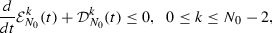
• (1) Taking $k=0,1,2,\ldots , N_0-2$, it follows that

  $$\begin{aligned} \mathcal {E}^k_{N_0}(t)\lesssim Y^2_0(1+t)^{-(\varrho +k)}. \end{aligned}$$

  (1.23)

• (2) Let $0\le i\le k\le N_0-3$ be an integer, if we take $l^*$ in Theorem 1.1 as $l^*=l'+\frac{3(\gamma +2s)}{2\gamma }+\chi _{N_0\ge 4}\left( 1-\frac{2s-1}{\gamma }\right) \left( N_0-4\right)$ and if we set $l_{0,0}=l_{0,1}=l_0$, $l_{0,k}+1+\frac{2s-1}{\gamma }= l_{0,k-1}$ and $l_{0,k}+\frac{(\gamma +2s)(k+2)}{2}\ge N_0$ for $2\le k\le N_0-3$, one has

  $$\begin{aligned} \mathcal {E}^k_{N_0,l_{0,k}+\frac{\gamma +2s}{2\gamma }i}(t) \lesssim Y^2_0(1+t)^{-k-\varrho +i}, \quad \quad i=0,1,\ldots ,k. \end{aligned}$$

  (1.24)

  furthermore, when $\varrho \in [1,\frac{3}{2})$,

  $$\begin{aligned} \mathcal {E}^k_{N_0,l_{0,k}+\frac{(\gamma +2s)(k+1)}{2\gamma }}(t) \lesssim Y^2_0(1+t)^{1-\varrho }.\quad \quad \quad \quad \quad \quad \quad \end{aligned}$$

  (1.25)

• (3) When $N_0+1\le |\alpha |\le N-1$, we have

  $$\begin{aligned} \Vert \partial ^\alpha f\Vert ^2 \lesssim Y^2_0(1+t)^{-\frac{(N-|\alpha |)(N_0-2+\varrho )}{N-N_0}}, \end{aligned}$$

  (1.26)

Remark 1.4

In fact, compared with the results in [5], the main results obtained in this manuscript show that:

• The smallness of $\Vert w_\ell f_0\Vert _{Z^1}$ and $\Vert (E_0,B_0)\Vert _{L^1}$ can be replaced by the weaker assumption that $\Vert (E_0,B_0)\Vert ^2_{\dot{H}^{-s}}+\Vert f_0\Vert ^2_{\dot{H}^{-s}}$ $(\frac{1}{2}<s<\frac{3}{2})$ is small.

• The minimal regularity index 14 is reduced into $N=7$ for $s\in (\frac{1}{2},1]$ and $N=6$ for $s\in (1,\frac{3}{2})$.

• The restriction on $\vartheta =\frac{1}{4}$ is relaxed to $0<\vartheta \le \frac{\varrho }{2}-\frac{1}{4}$, $\varrho \in (\frac{1}{2},\frac{3}{2})$ for $N_0\ge 4$ and $0<\vartheta \le \frac{\varrho }{2}-\frac{1}{2}, \varrho \in (1,\frac{3}{2})$ for $N_0=3$.

• The time decay rates of the higher-order spatial derivatives of solutions are obtained.

Let’s review some former results on the construction of global smooth solutions to the Vlasov–Maxwell–Boltzmann system (1.1) near Maxwellians. Guo in [9] firstly constructed periodic classical solutions near Maxwellian for the (non-relativistic) two-species Vlasov–Maxwell–Boltzmann system for hard sphere, which was extended to the whole space $\mathbb {R}^3_x$ by Strain in [18]. The large-time behavior of classical solutions to the Vlasov–Maxwell–Boltzmann system for hard sphere in the whole space was studied by Duan-Strain [6]. Recently, Duan-Liu-Yang-Zhao in [5] deal with the Vlasov–Maxwell–Boltzmann system for non-cutoff soft potentials in the whole space $\mathbb {R}^3_x$.

As pointed out in [5], to overcome the mathematical difficulties, which are produced by the velocity-growth of the nonlinear term with the velocity-growth rate |v| and the regularity-loss of the electromagnetic field, the main arguments used in [5] are as follows:

• They introduce the exponential time-velocity weight $w_\ell (t,v)$ to generate the extra dissipation corresponding to the last term in the energy dissipation rate functional $\mathcal {\bar{D}}_{N,l}(t)$;

• Motivated by the argument developed in [13] to deduce the decay property of solutions to nonlinear equations of regularity-loss type, a time-weighted energy estimate is designed to close the analysis, which implies that although the $L^2$-norm of terms with the highest order derivative with respect to x of the solutions of the Vlasov–Maxwell–Boltamann system may can only be bounded by some function of t which increases as time evolves, the $L^2$-norm of terms with lower order derivatives with respect to x still enjoy some decay rates.

Based on the above arguments and combining the decay of solutions to the corresponding linearized system with the Duhamel principle, Duan–Liu–Yang–Zhao [5] can indeed close the analysis provided that the regularity index imposed on the initial perturbation is 14, i.e. $N\ge 14$ and certain norms of the initial perturbation, especially $\Vert w_\ell f_0\Vert _{Z^1}$ and $\Vert (E_0,B_0)\Vert _{L^1}$, are assumed to be sufficiently small, meanwhile the choice of $\vartheta =\frac{1}{4}$ is critical in their proof.

Inspired by the work [11], the main purpose of our present manuscript is trying to study such a problem by a different method, which does not rely on the decay analysis of the corresponding linearized system and the Duhamel principle.

Now we sketch the main ideas to deduce our main results:

• As in [5], we apply the exponential time-velocity weight $w_\ell (t,v)$, which can deduce the extra dissipation $(1+t)^{-1-\vartheta }\Vert \langle v\rangle ^{\frac{1}{2}} w_\ell (\alpha ,\beta )\partial ^\alpha _\beta \{\mathbf{I-P}\}f\Vert ^2$, to control the term $\Vert E\Vert _{L^\infty }\Vert \langle v\rangle ^{\frac{1}{2}} w_\ell (\alpha ,\beta )\partial ^\alpha _\beta \{\mathbf{I-P}\}f\Vert ^2$. The key point of the above argument rests with the fact that the time decay rates of $\Vert E\Vert _{L^\infty }$ is greater than $1+\vartheta$. Unlike the techniques to obtain the time decay of $\Vert E\Vert _{L^\infty }$ in [5], which heavily rely on linear analysis and Duhamel principle, to deduce such a result, we hope that the following estimates

  

  (1.27)

  and

  

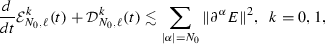  (1.28)

  hold for $0\le t<T$.

• In the proof of (1.27), the terms like $(\nabla ^k(v\cdot E {\mathbf P}f),\nabla ^k f)$ and $(\nabla ^k(v\times B\cdot \nabla _v {\mathbf P}f),\nabla ^k f)$ ask us to use the interpolation techniques between negative Sobolev norms i.e. $\Vert \Lambda ^{-\varrho }(f,E,B)\Vert$ and positive Sobolev norms i.e. $\Vert \nabla ^k\{\mathbf{I-P}\}f\Vert$ or $\Vert \nabla ^{k+1}({\mathbf P}f, E,B)\Vert$, and when we deal with the terms such as $(\nabla ^k(v\times B \nabla _v \{\mathbf{I- P}\}f),\nabla ^k \{\mathbf{I-P}\}f)$, even we have to apply the interpolation techniques with respect to velocity derivatives. In a word, the terms including electric–magnetic field (E,B) directly cause us to use the above techniques, which is mainly different from what Guo in [11] used to get the estimates like (1.27) with respect to Boltzmann equation (1.28) can be obtained in a similar way.

• With the help of the interpolation techniques between negative or the higher order Sobolev norms and corresponding dissipation functions introduced by [11], we deduce from (1.27) and (1.28) the time decay of $\mathcal {E}^k_{N_0}(t)$ and $\mathcal {E}^k_{N_0,\ell }(t)$. We notice that $\Vert E\Vert _{L^\infty }$ can be dominated by $\mathcal {E}^k_{N_0}(t)$ for $k=0,1,2$. Therefore, combing the time decay rates of $\Vert E\Vert _{L^\infty }$ and $\mathcal {E}^1_{N_0,\ell }(t)$ with other energy estimates, we can then close the a priori assumption given in (3.1) and then the global solvability result follows immediately from the continuation argument. It is worth pointing out that (1.27) and (1.28) play an essential role in the proof of Theorem 1.1.

The rest of this paper is organized as follows. In Sect. 2, we list some basic lemmas for the later proof. Section 3 is devoted to deducing the desired energy estimates for the energy functionals and the proofs of Theorems 1.1 and 1.3 will be given in the end of Sect. 3. For brevity, the detail proofs of some lemmas in Sect. 3 will be given in the Appendix.

2 Preliminary

In this section, we will cite some fundamental results for later use. The first lemma is concerned with the estimates of the linear operator L.

Lemma 2.1

(cf.[3, 5]) (i) It holds that

$$\begin{aligned} (Lg,g)\gtrsim \Vert \{{\mathbf {I}}-{\mathbf {P}}\}g\Vert _D^2. \end{aligned}$$

(2.1)

(ii) Let $\ell \in \mathbb {R}$, $\lambda \ge 0$, $0<s<1$ and $-3<\gamma <-2s$, it holds that

$$\begin{aligned} \sum _{|\beta |\le N}(w_{\ell }^{2}\partial _\beta Lg,\partial _\beta g)\gtrsim \Vert w_{\ell }\partial _\beta g\Vert _D^2-C\Vert g\Vert ^2_{L^2_{B_C}}. \end{aligned}$$

(2.2)

The second and third lemma concern the estimates on the nonlinear collision operator $\Gamma$.

Lemma 2.2

(cf. [3, 5]) For all $0<s<1$, $\max \big \{-3,-\frac{3}{2}-2s\big \}<\gamma <-2s$, $\lambda _0>0$ , $\ell \ge 0$ and for some $\bar{\lambda }>0$, then one has

$$\begin{aligned} \begin{aligned}&|\langle \partial _\beta ^\alpha \Gamma (f,g), w^2_{\ell }(\alpha ,\beta )\partial _\beta ^\alpha h\rangle |\\&\quad \lesssim \sum \left\{ \left| w_{\ell ,\lambda _0}\partial ^{\alpha _1}_{\beta _1}f\right| _{L^2_{s+\gamma /2}} \left| \partial ^{\alpha _2}_{\beta _2}g\right| _D+\left| \partial ^{\alpha _2}_{\beta _2}g\right| _{L^2_{s+\gamma /2}} \left| w_\ell (\alpha ,\beta )\partial ^{\alpha _1}_{\beta _1}f\right| _D\right\} \left| w_\ell (\alpha ,\beta )\partial ^{\alpha }_{\beta }h\right| _D\\&\qquad +\min \left\{ \left| w_\ell (\alpha ,\beta )\partial ^{\alpha _1}_{\beta _1}f\right| _{L^2} \left| \partial ^{\alpha _2}_{\beta _2}g\right| _{L^2_{s+\gamma /2}},\left| \partial ^{\alpha _2}_{\beta _2}g\right| _{L^2} \left| w_\ell (\alpha ,\beta )\partial ^{\alpha _1}_{\beta _1}f\right| _{L^2_{s+\gamma /2}}\right\} \left| w_\ell (\alpha ,\beta )\partial ^{\alpha }_{\beta }h\right| _D\\&\qquad +\sum \left| e^{\frac{\lambda _0\langle v\rangle }{(1+t)^{\vartheta }}}\partial ^{\alpha _2}_{\beta _2}g\right| _{L^2} \left| w_\ell (\alpha ,\beta )\partial ^{\alpha _1}_{\beta _1}f\right| _{L^2_{\gamma /2}} \left| w_\ell (\alpha ,\beta )\partial ^{\alpha }_{\beta }h\right| _D\\&\qquad +\sum \left| \mu ^{\frac{\bar{\lambda }}{128}}\partial ^{\alpha _2}_{\beta _2}g\right| _{L^2} \left| w_\ell (\alpha ,\beta )\partial ^{\alpha _1}_{\beta _1}f\right| _{L^2_{\gamma /2+1/2}} \left| w_\ell (\alpha ,\beta )\partial ^{\alpha }_{\beta }h\right| _{L^2_{\gamma /2+1/2}}\\&\qquad +\sum (1+t)^{-\vartheta }\left| \mu ^{\frac{\bar{\lambda }}{128}}\partial ^{\alpha _2}_{\beta _2}g\right| _{L^2} \left| w_\ell (\alpha ,\beta )\partial ^{\alpha _1}_{\beta _1}f\right| _{L^2_{\gamma /2+1}} \left| w_\ell (\alpha ,\beta )\partial ^{\alpha }_{\beta }h\right| _{L^2_{\gamma /2+s}}\\&\qquad +\sum (1+t)^{-2\vartheta }\left| \mu ^{\frac{\bar{\lambda }}{128}}\partial ^{\alpha _2}_{\beta _2}g\right| _{L^2} \left| w_\ell (\alpha ,\beta )\partial ^{\alpha _1}_{\beta _1}f\right| _{L^2_{\gamma /2+1}} \left| w_\ell (\alpha ,\beta )\partial ^{\alpha }_{\beta }h\right| _{L^2_{\gamma /2+1}}, \end{aligned} \end{aligned}$$

(2.3)

where the summation $\sum$ is taken over $\alpha _1+\alpha _2\le \alpha$ and $\beta _1+\beta _2\le \beta$. Furthermore, from [3],

$$\begin{aligned} |\langle \Gamma (f,g), h\rangle |\lesssim \left\{ |f|_{L^2_{\gamma /2+s}}|g|_D+|g|_{L^2_{\gamma /2+s}}|f|_D+\min \left\{ |f|_{L^2}|g|_{L^2_{\gamma /2+s}},|g|_{L^2}|f|_{L^2_{\gamma /2+s}}\right\} \right\} |h|_D.\nonumber \\ \end{aligned}$$

(2.4)

Lemma 2.3

(cf. [19]) Let $\ell >0$, $\gamma >-3$ with $\gamma +2s>-\frac{3}{2}$ and $s\in [\frac{1}{2},1)$, it holds that

$$\begin{aligned} |w_\ell \Gamma (f,f)|_{L^2}\lesssim |w_\ell f|^2_{L^2_{\gamma /2+s}}|w_\ell f|^2_{H^2_{\gamma /2+s}}. \end{aligned}$$

(2.5)

The following lemma concerns the trillion estimates on the nonlinear term $\Gamma (f,f)$.

Lemma 2.4

For all $\frac{1}{2}\le s<1$, $\max \big \{-3,-\frac{3}{2}-2s\big \}<\gamma <-2s$, and assume $\ell \ge N$, $0<\vartheta \le \frac{1}{3}$, one has the following estimates:

$$\begin{aligned} \sum _{|\alpha |\le N}\left| \left( \partial ^\alpha \Gamma (f,f), \partial ^\alpha \mathbf{\{I-P\}}f\right) \right|\lesssim & {} \mathcal {E}^{1/2}_{N_0,N_0}(t)\mathcal {D}_{N}(t),\end{aligned}$$

(2.6)

$$\begin{aligned} \left| \left( w^2_\ell (0,0)\Gamma (f,f), \mathbf{\{I-P\}}f\right) \right|\lesssim & {} (1+t)^{\frac{1-3\vartheta }{2}}\big \{\mathcal {E}^1_{N_0,\ell -N_0+2}(t)\big \}^{1/2}\mathcal {D}_{N,\ell }(t)\nonumber \\&+\,\mathcal {E}^{1/2}_{N_0,N_0}(t)\mathcal {D}_{N,\ell }(t),\end{aligned}$$

(2.7)

$$\begin{aligned} \sum _{0<|\alpha |\le N_0}\left| \left( w^2_\ell (\alpha ,0)\partial ^\alpha \Gamma (f,f), \partial ^\alpha f\right) \right|\lesssim & {} (1+t)^{\frac{1-3\vartheta }{2}}\big \{\mathcal {E}^1_{N_0,\ell -N_0+2}(t)\big \}^{1/2}\mathcal {D}_{N,\ell }(t)\nonumber \\&+\,\mathcal {E}^{1/2}_{N_0,N_0}(t)\mathcal {D}_{N,\ell }(t), \end{aligned}$$

(2.8)

and

$$\begin{aligned} \sum _{\begin{array}{c} {|\alpha |+|\beta |\le N_0},\\ {|\beta |\ge 1} \end{array}}\left| \left( w^2_\ell (\alpha ,\beta )\partial ^\alpha _\beta \Gamma (f,f), \partial ^\alpha _\beta \mathbf{\{I-P\}}f\right) \right|\lesssim & {} (1+t)^{\frac{1-3\vartheta }{2}}\big \{\mathcal {E}^1_{N_0,\ell -N_0+2}(t)\big \}^{1/2}\mathcal {D}_{N,\ell }(t)\nonumber \\&+\,\mathcal {E}^{1/2}_{N_0,N_0}(t)\mathcal {D}_{N,\ell }(t). \end{aligned}$$

(2.9)

Proof

For brevity, we only prove (4.3),

$$\begin{aligned} \begin{aligned}&|\left( \partial ^\alpha \Gamma (f,f), w_\ell (\alpha ,0)^2\partial ^\alpha f\right) |\\&\quad \lesssim \int _{\mathbb {R}^3}\sum \left\{ \left| w_\ell (\alpha ,0)\partial ^{\alpha _1}f\right| _{L^2_{s+\gamma /2}} \left| \partial ^{\alpha _2}f\right| _D+\left| \partial ^{\alpha _2}f\right| _{L^2_{s+\gamma /2}} \left| w_\ell (\alpha ,0)\partial ^{\alpha _1}f\right| _D\right\} \\&\qquad \times \left| w_\ell (\alpha ,0)\partial ^{\alpha }f\right| _D dx\\&\qquad +\int _{\mathbb {R}^3}\min \left\{ \left| w_\ell (\alpha ,0)\partial ^{\alpha _1}f\right| _{L^2} \left| \partial ^{\alpha _2}f\right| _{L^2_{s+\gamma /2}},\left| \partial ^{\alpha _2}f\right| _{L^2} \left| w_\ell (\alpha ,0)\partial ^{\alpha _1}f\right| _{L^2_{s+\gamma /2}}\right\} \\&\qquad \times \left| w_\ell (\alpha ,0)\partial ^{\alpha }f\right| _Ddx\\&\qquad +\int _{\mathbb {R}^3}\sum \left| e^{\frac{\lambda _0\langle v\rangle }{(1+t)^{\vartheta }}}\partial ^{\alpha _2}f\right| _{L^2} \left| w_\ell (\alpha ,0)\partial ^{\alpha _1}f\right| _{L^2_{\gamma /2}} \left| w_\ell (\alpha ,0)\partial ^{\alpha }f\right| _Ddx\\&\qquad +\int _{\mathbb {R}^3}\sum \left| \mu ^{\frac{\bar{\lambda }}{128}}\partial ^{\alpha _2}f\right| _{L^2} \left| w_\ell (\alpha ,0)\partial ^{\alpha _1}f\right| _{L^2_{\gamma /2+1/2}} \left| w_\ell (\alpha ,0)\partial ^{\alpha }f\right| _{L^2_{\gamma /2+1/2}}dx\\&\qquad +\int _{\mathbb {R}^3}\sum (1+t)^{-\vartheta }\left| \mu ^{\frac{\bar{\lambda }}{128}}\partial ^{\alpha _2}f\right| _{L^2} \left| w_\ell (\alpha ,0)\partial ^{\alpha _1}f\right| _{L^2_{\gamma /2+1}} \left| w_\ell (\alpha ,0)\partial ^{\alpha }f\right| _{L^2_{\gamma /2+s}}dx\\&\qquad +\int _{\mathbb {R}^3}\sum (1+t)^{-2\vartheta }\left| \mu ^{\frac{\bar{\lambda }}{128}}\partial ^{\alpha _2}f\right| _{L^2} \left| w_\ell (\alpha ,0)\partial ^{\alpha _1}f\right| _{L^2_{\gamma /2+1}} \left| w_\ell (\alpha ,0)\partial ^{\alpha }f\right| _{L^2_{\gamma /2+1}}dx\\&\qquad \equiv \sum _{i=1}^6R_i, \end{aligned} \end{aligned}$$

(2.10)

where we should notice the summation $\sum$ is taken over $\alpha _1+\alpha _2\le \alpha$. We only prove the last term on right hand of (2.10) since the estimates for the other terms on the right hand of (2.10) are more simple than the last term. Since $\gamma \le -2s$ and $1/2\le s<1$, we see that $\gamma +2\le 1$. Therefore,

$$\begin{aligned} (1+t)^{-(1+\vartheta )}\Vert \langle v\rangle ^{\gamma /2+1}w_\ell (\alpha ,\beta )\partial ^\alpha _\beta \mathbf{\{I-P\}}f\Vert ^2\lesssim \mathcal {D}_{N,\ell }(t). \end{aligned}$$

(2.11)

When $\alpha _2=\alpha$ with $|\alpha |\ge N_0+1$, we use $L^2-L^\infty -L^2$,

$$\begin{aligned} \begin{aligned}&\int _{\mathbb {R}^3}(1+t)^{-2\vartheta }\left| \mu ^{\frac{\bar{\lambda }}{128}}\partial ^{\alpha }f\right| _{L^2} \left| w_\ell (\alpha ,0)f\right| _{L^2_{\gamma /2+1}} \left| w_\ell (\alpha ,0)\partial ^{\alpha }f\right| _{L^2_{\gamma /2+1}}dx\\&\quad \lesssim \,(1+t)^{-2\vartheta }\Vert \mu ^\delta \partial ^{\alpha }f\Vert \left\| w_\ell (\alpha ,0)\nabla f\right\| _{H^1_xL^2_{\gamma /2+1}}\left\| w_\ell (\alpha ,0)\partial ^{\alpha }f\right\| _{L^2_{\gamma /2+1}}\\&\quad \lesssim \,(1+t)^{\frac{1-3\vartheta }{2}}\big \{\mathcal {E}_{N_0,\ell -N_0+2}(t)\big \}^{1/2}\mathcal {D}_{N,\ell }(t). \end{aligned} \end{aligned}$$

(2.12)

When $N_0+1\le |\alpha _2|\le |\alpha |-1$ with $|\alpha |\ge N_0+2$, we use $L^3-L^6-L^2$,

$$\begin{aligned} \begin{aligned}&\int _{\mathbb {R}^3}(1+t)^{-2\vartheta }\left| \mu ^{\frac{\bar{\lambda }}{128}}\partial ^{\alpha _2}f\right| _{L^2} \left| w_\ell (\alpha ,0)\partial ^{\alpha _1}f\right| _{L^2_{\gamma /2+1}} \left| w_\ell (\alpha ,0)\partial ^{\alpha }f\right| _{L^2_{\gamma /2+1}}dx\\&\quad \lesssim \,(1+t)^{-2\vartheta }\Vert \mu ^\delta \partial ^{\alpha _2}f\Vert \left\| w_\ell (\alpha ,0)\nabla \partial ^{\alpha _1}f\right\| _{L^2_{\gamma /2+1}}\left\| w_\ell (\alpha ,0)\partial ^{\alpha }f\right\| _{L^2_{\gamma /2+1}}\\&\quad \lesssim \,(1+t)^{\frac{1-3\vartheta }{2}}\big \{\mathcal {E}_{N_0,\ell -N_0+2}(t)\big \}^{1/2}\mathcal {D}_{N,\ell }(t). \end{aligned} \end{aligned}$$

(2.13)

Collecting the above estimates yields $R_6\lesssim (1+t)^{\frac{1-3\vartheta }{2}}\{\mathcal {E}_{N_0,\ell -N_0+2}(t)\}^{1/2} \mathcal {D}_{N,\ell }(t)+\{\mathcal {E}_{N_0,N_0}(t)\}^{1/2}\mathcal {D}_{N,\ell }(t).$

For other terms $R_1\sim R_5$, noticing that $0<\vartheta \le \frac{1}{3}$, we can obtain easily by the similar way as $R_6$

$$\begin{aligned} \begin{aligned} \sum _{i=1}^{5}R_i\lesssim (1+t)^{\frac{1-3\vartheta }{2}}\big \{\mathcal {E}^1_{N_0,\ell -N_0+2}(t)\big \}^{1/2}\mathcal {D}_{N,\ell }(t) +\mathcal {E}^{1/2}_{N_0,N_0}(t)\mathcal {D}_{N,\ell }(t). \end{aligned} \end{aligned}$$

Collecting the above estimates gives (4.3) for the case $N_0+1\le |\alpha |\le N$. While for the case $|\alpha |\le N_0$, (4.3) can be obtained in a similar way. Thus we have completed the proof of this lemma. $\square$

In what follows, we will collect the analytic tools which will be used in this paper. The Sobolev interpolation among the spatial regularity is

Lemma 2.5

(cf. [21]) Let $2\le p<\infty$ and $k,\ell , m\in \mathbb {R}$; then we have

$$\begin{aligned} \Vert \nabla ^k f\Vert _{L^p}\lesssim \Vert \nabla ^\ell f\Vert ^{\theta }_{L^2}\Vert \nabla ^m f\Vert ^{1-\theta }_{L^2}. \end{aligned}$$

(2.14)

where $0\le \theta \le 1$ and $\ell$ satisfy

$$\begin{aligned} \frac{1}{p}-\frac{k}{3}=\left( \frac{1}{2}-\frac{\ell }{3}\right) \theta +\left( \frac{1}{2}-\frac{m}{3}\right) (1-\theta ). \end{aligned}$$

(2.15)

Also we have that

$$\begin{aligned} \Vert \nabla ^k f\Vert _{L^\infty }\lesssim \Vert \nabla ^\ell f\Vert ^{\theta }_{L^2}\Vert \nabla ^m f\Vert ^{1-\theta }_{L^2}. \end{aligned}$$

(2.16)

where $0\le \theta \le 1$ and $\ell$ satisfy

$$\begin{aligned} -\frac{k}{3}=\left( \frac{1}{2}-\frac{\ell }{3}\right) \theta +\left( \frac{1}{2}-\frac{m}{3}\right) (1-\theta ), \end{aligned}$$

(2.17)

here we require $\ell \le k+1$ and $m\ge k+2$.

In this paper, we should estimate $\Vert \Lambda ^{-\varrho }f\Vert$, we need the following $L^p$ inequality for $\Lambda ^{-\varrho }$.

Lemma 2.6

(cf. [11, 17]) Let $0<\varrho <3$, $1<p<q<\infty$, $\frac{1}{q}+\frac{\varrho }{3}=\frac{1}{p}$, then

$$\begin{aligned} \Vert \Lambda ^{-\varrho }f\Vert _{L^q}\lesssim \Vert f\Vert _{L^p}. \end{aligned}$$

(2.18)

In many places, we will use Minkowski’s integral inequality to interchange the orders of integration over x and v.

Lemma 2.7

(cf. [21]) For $1\le p\le q\le \infty$, we have

$$\begin{aligned} \Vert f\Vert _{L^q_zL^p_y}\le \Vert f\Vert _{L^p_yL^q_z}. \end{aligned}$$

(2.19)

3 The Proofs of Our Main Results

This section is devoted to proving our main results based on the continuation argument. For this purpose, suppose that the Cauchy problem (1.4) and (1.5) admits a unique local solution f(t, x, v) defined on the time interval $0\le t\le T$ for some $0<T<\infty$ and the solution f(t, x, v) satisfies the a priori assumption

$$\begin{aligned} \begin{aligned} X(t)=\sup _{0\le \tau \le t}\left\{ \bar{\mathcal {E}}_{N_0,l_0+l^*}(\tau )+\mathcal {E}_{N}(\tau )+\mathcal {E}_{N-1,l}(\tau )+(1+\tau )^{-\frac{1+\epsilon _0}{2}}\mathcal {E}_{N,l}(\tau )\right\} \le M, \end{aligned} \end{aligned}$$

(3.1)

where the parameters $N_0,N,l, l_0,$ and $l^*$ are given in Theorem 1.1 and M is a sufficiently small positive constant. Then use the continuation argument to extend such a solution step by step to a global one, one only need to deduce certain uniform-in-time energy type estimates on f(t, x, v) such that the a priori assumption (3.1) can be closed.

For this purpose, we first deduce the temporal decay of the energy functional $\mathcal {E}^k_{N_0}(t)$ in the following lemma.

Lemma 3.1

Let $N_0$ and N satisfy (1.21), $n\ge \frac{2}{3} N_0-\frac{5}{3}$, and take $k=0,1,2,\ldots , N_0-2$, then one has

(3.2)

provided that

$$\begin{aligned} (H_1) \quad \quad&\max \left\{ \displaystyle \sup _{0\le \tau \le T}\mathcal {E}_{N_0+n}(\tau ), \sup _{0\le \tau \le T}\mathcal {E}_{N-1,N-1}(\tau ), \sup _{0\le \tau \le T}\mathcal {\overline{E}}_{N_0,N_0+l'}(\tau )\right\} \\&\quad \ is\ \ sufficiently\ \ small. \end{aligned}$$

Furthermore, as a consequence of (3.2), we can get that

$$\begin{aligned} \mathcal {E}^k_{N_0}(t)\lesssim \max \left\{ \sup _{0\le \tau \le t}\mathcal {\overline{E}}_{N_0,N_0+\frac{\gamma +2s}{2\gamma }}(\tau ),\sup _{0\le \tau \le t}\mathcal {E}_{N_0+k+\varrho }(\tau )\right\} (1+t)^{-(k+\varrho )} \end{aligned}$$

(3.3)

holds for $0\le t\le T$.

Proof

Under the smallness assumption $(H_1)$, one can deduce that

which is a immediately consequence of Lemma 4.1 and Lemma 4.2 whose proofs are postponed to the next section for simplicity, where we used the fact that $\overline{m}$ of Lemma 4.1 is less or equal to $N-1$.

To get (3.3), for the macroscopic component ${\mathbf P}f(t,x,v)$ and the electromagnetic field [E(t, x), B(t, x)] one has by Lemma 2.5 that

$$\begin{aligned} \begin{aligned} \left\| \nabla ^k({\mathbf P}f,B)\right\| \le \left\| \nabla ^{k+1}({\mathbf P}f,B)\right\| ^{\frac{k+\varrho }{k+\varrho +1}}\left\| \Lambda ^{-\varrho }({\mathbf P}f,B)\right\| ^{\frac{1}{k+\varrho +1}} \end{aligned} \end{aligned}$$

and

$$\begin{aligned} \left\| \nabla ^{N_0}(E,B)\right\| \lesssim \left\| \nabla ^{N_0-1}(E,B)\right\| ^\frac{k+\varrho }{k+\varrho +1} \left\| \nabla ^{N_0+k+\varrho }(E,B)\right\| ^\frac{1}{k+\varrho +1}, \end{aligned}$$

while for the microscopic component $\{\mathbf{I}-\mathbf{P}\}f(t,x,v)$, employing the Hölder inequality gives

$$\begin{aligned} \begin{aligned} \sum _{k\le |\alpha |\le N_0}\left\| \partial ^\alpha \mathbf{\{I-P\}}f\right\| \le&\left\| \partial ^\alpha \mathbf{\{I-P\}}f\langle v\rangle ^{\frac{\gamma +2s}{2}}\right\| ^{\frac{k+\varrho }{k+\varrho +1}} \left\| \partial ^\alpha \mathbf{\{I-P\}}f\langle v\rangle ^{-\frac{{(\gamma +2s)}(k+\varrho )}{2}}\right\| ^{\frac{1}{k+\varrho +1}}\\ \le&\left\| \partial ^\alpha \mathbf{\{I-P\}}f\right\| _\nu ^{\frac{k+\varrho }{k+\varrho +1}} \left\| w_{|\alpha |+\frac{\gamma +2s}{2\gamma }}\partial ^\alpha \mathbf{\{I-P\}}f\right\| ^{\frac{1}{k+\varrho +1}}. \end{aligned} \end{aligned}$$

Thus, we have

$$\begin{aligned} \begin{aligned} \mathcal {E}^k_{N_0}(t)\le \left\{ \mathcal {D}^k_{N_0}(t)\right\} ^\frac{k+\varrho }{k+\varrho +1}\left\{ \max \left\{ \sup _{0\le \tau \le t}\mathcal {\overline{E}}_{N_0,N_0+\frac{\gamma +2s}{2\gamma }}(\tau ),\sup _{0\le \tau \le t}\mathcal {E}_{N_0+k+\varrho }(\tau )\right\} \right\} ^\frac{1}{k+\varrho +1}, \end{aligned} \end{aligned}$$

which combing with (3.2) yields that

Solving the above inequality directly gives

$$\begin{aligned} \mathcal {E}^k_{N_0}(t)\lesssim \max \left\{ \sup _{0\le \tau \le t}\mathcal {\overline{E}}_{N_0,N_0+\frac{\gamma +2s}{2\gamma }}(\tau ),\sup _{0\le \tau \le t}\mathcal {E}_{N_0+k+\varrho }(\tau )\right\} (1+t)^{-(k+\varrho )}. \end{aligned}$$

This completes the proof of Lemma 3.1. $\square$

Lemma 3.2

Let $\ell \ge N_0$, $n\ge \frac{2}{3} N_0-\frac{5}{3}$ and suppose that

$$\begin{aligned} (H_2) \quad \quad \max \left\{ \sup \limits _{0\le \tau \le t}\mathcal {E}_{N_0+n}(\tau ), \sup \limits _{0\le \tau \le t}\mathcal {E}_{N_0,\ell }(\tau )\right\} \ \ is\ \ sufficiently\ \ small \end{aligned}$$

with $\widetilde{l}$ being given in Lemma 3.1,

(3.4)

for any $0\le t\le T$, where $k=0,1,\ldots ,N_0-3$. Furthermore, based on (3.4), if we set $l_{0,0}=l_{0,1}=\ell$, $l_{0,k}+1+\frac{2s-1}{\gamma }= l_{0,k-1}$ and $l_{0,k}+\frac{(\gamma +2s)(k+2)}{2}\ge N_0$ for $2\le k\le N_0-3$, we can deduce

$$\begin{aligned} \mathcal {E}^k_{N_0,l_{0,k}+\frac{\gamma +2s}{2\gamma }i}(t) \lesssim X(t)(1+t)^{-k-\varrho +i}, \quad \quad i=0,1,\ldots ,k, \end{aligned}$$

(3.5)

while for $\varrho \in [1,3/2)$,

$$\begin{aligned} \mathcal {E}^k_{N_0,l_{0,k}+\frac{(\gamma +2s)(k+1)}{2\gamma }}(t) \lesssim X(t)(1+t)^{1-\varrho }, \end{aligned}$$

(3.6)

Proof

Since the proof of (3.4) is nearly same to (3.2), we only point out the main difference between the proof of (3.4) and (3.2). For instance, when $|\alpha |= N_0$, one has

$$\begin{aligned} \begin{aligned}&(v\times \partial ^{e_i}B \partial ^{\alpha -e_i}\nabla _v\{\mathbf{I-P}\}f, w_\ell (\alpha ,0)^2 \partial ^{\alpha }\{\mathbf{I-P}\}f)\\&\quad \lesssim \Vert \nabla B\Vert ^2_{L^\infty }\Vert w_\ell (\alpha ,0)\partial ^{\alpha -e_i}\nabla _v\{\mathbf{I-P}\}f\langle v\rangle ^{1-\frac{\gamma }{2}-s}\Vert ^2+\varepsilon \Vert w_\ell (\alpha ,\beta )\partial ^{\alpha }\{\mathbf{I-P}\}f\Vert _D^2 \end{aligned} \end{aligned}$$

(3.7)

which will be included on the right hand side of (3.4) for $k\ge 2$.

For $k=0,1$, multiplying (3.4) with $\ell =l_0+\frac{\gamma +2s}{2\gamma }i$ by $(1+t)^{k+\varrho -i+\epsilon }$ gives

(3.8)

where $\epsilon$ is taken as a sufficiently small positive constant. When $\varrho \in (1/2,1)$, we take $\ell =l_{0,k}+\frac{(\gamma +2s)(k+1)}{2\gamma }$ in (3.4), it holds that

(3.9)

Using the relation between the energy functional $\mathcal {E}^k_{N_0,\ell }(t)$ and its dissipation rate $\mathcal {D}^k_{N_0,\ell }(t)$, the proper linear combination of (3.8) and (3.9) yields

(3.10)

Lemma 3.1 tells us that

$$\begin{aligned} \begin{aligned} \sum _{|\alpha |=N_0}(1+t)^{k+\varrho +\epsilon }\Vert \partial ^\alpha E\Vert ^2\,+\,&(1+t)^{k+\varrho -1+\epsilon }\Vert \nabla ^k({\mathbf P}f,E,B)\Vert ^2\lesssim X(t)(1+t)^{-1+\epsilon }. \end{aligned} \end{aligned}$$

(3.11)

Plugging (3.11) into (3.10) and taking the time integration, it follows that

$$\begin{aligned} \begin{aligned}&\sum _{i=0}^k(1+t)^{k+\varrho -i+\epsilon }\mathcal {E}^k_{N_0,l_{0,k}+\frac{\gamma +2s}{2\gamma }i}(t)+\mathcal {E}^k_{N_0,l_{0,k}+\frac{(\gamma +2s)(k+1)}{2\gamma }}(t)\\&\quad +\int _0^t\left( \sum _{i=0}^k(1+t)^{k+\varrho -i+\epsilon }\mathcal {D}^k_{N_0,l_{0,k}+\frac{\gamma +2s}{2\gamma }i}(\tau )+\mathcal {D}^k_{N_0,l_{0,k}+\frac{(\gamma +2s)(k+1)}{2\gamma }}(\tau )\right) d\tau \lesssim X(t)(1+t)^{\epsilon }. \end{aligned} \end{aligned}$$

(3.12)

Using this, it follows that

$$\begin{aligned} \mathcal {E}^k_{N_0,l_{0,k}+\frac{\gamma +2s}{2\gamma }i}(t) \lesssim X(t)(1+t)^{-k-\varrho +i}, \quad \quad i=0,1,\ldots ,k. \end{aligned}$$

(3.13)

When $\varrho \in [1,3/2)$, multiplying (3.4) with $\ell =l_{0,k}+\frac{(\gamma +2s)(k+1)}{2\gamma }$ by $(1+t)^{\varrho -1+\epsilon }$ gives

(3.14)

we take $\ell =l_{0,k}+\frac{(\gamma +2s)(k+2)}{2\gamma }$ in (3.4), it holds that

(3.15)

As in the case $\varrho \in (\frac{1}{2},1)$, the proper linear combination of (3.8), (3.14) and (3.14) yields

(3.16)

By the same way as (3.5), it follows that

$$\begin{aligned} \begin{aligned}&\sum _{i=0}^{k+1}(1+t)^{k+\varrho -i+\epsilon }\mathcal {E}^k_{N_0,l_{0,k}+\frac{\gamma +2s}{2\gamma }i}(t)+\mathcal {E}^k_{N_0,l_{0,k}+\frac{(\gamma +2s)(k+2)}{2\gamma }}(t)\\&\quad +\int _0^t\left( \sum _{i=0}^{k+1}(1+t)^{k+\varrho -i+\epsilon }\mathcal {D}^k_{N_0,l_{0,k}+\frac{\gamma +2s}{2\gamma }i}(\tau )+\mathcal {D}^k_{N_0,l_{0,k}+\frac{(\gamma +2s)(k+2)}{2\gamma }}(\tau )\right) d\tau \lesssim X(t)(1+t)^{\epsilon }. \end{aligned} \end{aligned}$$

(3.17)

Combining (3.12) and (3.17) yields (3.5) and (3.6).

When $k\ge 2$, we let $l_{0,0}=l_{0,1}=\ell$, by using the principle of mathematical induction, we can get that

$$\begin{aligned} \mathcal {E}^k_{N_0,l_{0,k}+\frac{\gamma +2s}{2\gamma }i}(t) \lesssim X(t)(1+t)^{-k-\varrho +i}, \quad \quad \varrho \in \left( 1/2,3/2\right) \quad \quad i=0,1,\ldots ,k. \end{aligned}$$

(3.18)

especially, when $\varrho \in [1,3/2)$,

$$\begin{aligned} \mathcal {E}^k_{N_0,l_{0,k}+\frac{(\gamma +2s)(k+1)}{2\gamma }}(t) \lesssim X(t)(1+t)^{1-\varrho },\quad \quad \quad \quad \end{aligned}$$

(3.19)

where $l_{0,k}+1+\frac{2s-1}{\gamma }=l_{0,k-1}$. This completes the proof of Lemma 3.2. $\square$

Bases on the time decay estimates on $\mathcal {E}^k_{N_0}(t)$ and $\mathcal {E}^k_{N_0,\ell }(t)$, and suppose $\displaystyle \max \left\{ \sup \nolimits _{0\le t\le T}\mathcal {E}_{N_0,N_0}(t),\sup \nolimits _{0\le t\le T}\mathcal {E}_{N}(t)\right\}$ is sufficiently small, we will have the following three lemmas for $\mathcal {E}_{N}(t),\mathcal {E}_{N,l}(t),\mathcal {E}_{N-1,l}(t)$ and $\mathcal {\bar{E}}_{N_0,l_0+l*}(t)$ respectively:

Lemma 3.3

Let $N_0, N$ and $\vartheta$ satisfy (1.21) and (1.10) respectively, under the assumptions of Lemma 3.1 and $l\ge N$, $l_0\ge N-N_0+\frac{1}{2}-\frac{1-s}{\gamma }$, we can deduce that

(3.20)

holds for all $0\le t\le T$.

Proof

First of all, it is straightforward to establish the energy identities

$$\begin{aligned}&\frac{1}{2}\frac{d}{dt}\sum \limits _{N_0+1\le |\alpha |\le N}\left( \left\| \partial ^\alpha f\right\| ^2+ \left\| \partial ^\alpha (E,B)\right\| ^2\right) +\sum \limits _{N_0+1\le |\alpha |\le N}\left( L\partial ^\alpha f,\partial ^\alpha f\right) \nonumber \\&\quad =\underbrace{\sum \limits _{N_0+1\le |\alpha |\le N}\left( \partial ^\alpha \left( \frac{q_0}{2}E\cdot vf\right) ,\partial ^\alpha f\right) }_{J_1}-\underbrace{\sum \limits _{N_0+1\le |\alpha |\le N}\left( \partial ^\alpha \left( q_0(E+v\times B)\cdot \nabla _vf\right) ,\partial ^\alpha f\right) }_{J_2}\nonumber \\&\quad +\underbrace{\sum \limits _{N_0+1\le |\alpha |\le N}\left( \partial ^\alpha \Gamma (f,f),\partial ^\alpha f\right) }_{J_3}. \end{aligned}$$

(3.21)

For the $\partial ^\alpha$ derivative term related to (E, B) with $N_0+1\le |\alpha |\le N$, i.e., the estimates on $J_1$ and $J_2$, one has

$$\begin{aligned} \begin{aligned} J_1&\lesssim \Vert E\Vert _{L^\infty } \left\| \langle v\rangle ^{1/2}\partial ^{\alpha }f\right\| \left\| \langle v\rangle ^{1/2}\partial ^\alpha f\right\| \\&\quad +\sum _{1\le |\alpha _1|\le N_0-1}\left\| \partial ^{\alpha _1}E\right\| _{L^6} \left\| \langle v\rangle ^{1/2}\partial ^{\alpha -\alpha _1}f\right\| _{L^3} \left\| \langle v\rangle ^{1/2}\partial ^\alpha f\right\| \\&\quad +\sum _{|\alpha _1|= N_0}\left\| \partial ^{\alpha _1}E\right\| \left\| \langle v\rangle ^{1/2}\partial ^{\alpha -\alpha _1}f\right\| _{L^\infty } \left\| \langle v\rangle ^{1/2}\partial ^\alpha f\right\| \\&\quad +\sum _{|\alpha _1|\ge N_0+1,\alpha _1\ne \alpha }\left\| \partial ^{\alpha _1}E\right\| _{L^6} \left\| \langle v\rangle ^{1-s-\frac{\gamma }{2}}\partial ^{\alpha -\alpha _1}f\right\| _{L^3} \left\| \partial ^\alpha f\right\| _D\\&\quad +\left\| \partial ^{\alpha }E\right\| \left\| \langle v\rangle ^{1-s-\frac{\gamma }{2}}f\right\| _{L^\infty } \left\| \partial ^\alpha f\right\| _D\\ \lesssim&\left( \Vert E\Vert _{L^{\infty }}+\left\| \nabla ^2E\right\| _{H^{ N_0-2}}\right) \mathcal {D}_{N,l}(t) +\mathcal {E}_N(t)\mathcal {E}^1_{N_0,l_0}(t)+\varepsilon \mathcal {D}_{N}(t). \end{aligned} \end{aligned}$$

(3.22)

For $J_2$, due to $\left( (E+v\times B)\cdot \partial ^\alpha \nabla _vf,\partial ^\alpha f\right) =0,$ we can deduce by employing the same argument to deal with $J_1$ that

$$\begin{aligned} J_2\lesssim \left\| \nabla ^2(E,B)\right\| _{H^{ N_0-2}}\mathcal {D}_{N,l}(t) +\mathcal {E}_N(t)\mathcal {E}^1_{N_0,l_0}(t) +\varepsilon \mathcal {D}_{N}(t). \end{aligned}$$

Here we choose $l_0\ge N-N_0+\frac{1}{2}-\frac{1-s}{\gamma }$ and $N\le 2N_0$. It follows from Lemma 2.2 that $J_3\lesssim (\mathcal {E}_N(t)+\varepsilon )\mathcal {D}_N(t).$

Plugging the estimates of $J_1,\ J_2,\ J_3$ into (3.21) yields

(3.23)

which combining with (3.2) and (4.35) give the proof of (3.20) under the assumptions (1.10). $\square$

Lemma 3.4

Let $N_0, N$ and $\vartheta$ satisfy (1.21) and (1.10) respectively,, we can deduce that

(3.24)

holds for all $0\le t\le T$.

Proof

The proof of this lemma is divided into two steps. The first step is to deduce the desired energy type estimates on the derivatives of f(t, x, v) with respect to the x-variable only. For this purpose, the standard energy estimate on $\partial ^\alpha f$ with $1\le |\alpha |\le N$ weighted by the time-velocity dependent function $w_{l}(\alpha ,0)=w_l(\alpha ,0)(t,v)$ gives

(3.25)

As to the estimates on $J_4$, $J_5$, and $J_6$, we can deduce by following exactly the argument used above to control $J_1$, $J_2$, and $J_3$ that

$$\begin{aligned} \begin{aligned} J_4+J_5\lesssim&(1+t)^{1+\vartheta }\left( \Vert E\Vert _{L^{\infty }} +\left\| \nabla ^2_x(E,B)\right\| _{H^{ N_0-2}}\right) \mathcal {D}_{N,l}(t) +\mathcal {E}_N(t)\mathcal {E}^1_{N_0,l_0}(t)+\varepsilon \mathcal {D}_{N,l}(t), \end{aligned} \end{aligned}$$

(3.26)

and using Lemma 2.2 gives

$$\begin{aligned} \begin{aligned}&J_6\lesssim (1+t)^{\frac{1-3\vartheta }{2}}\mathcal {E}^1_{N_0,l-N_0+2}(t)^{1/2}\mathcal {D}_{N,l}(t) +\mathcal {E}^{1/2}_{N_0,N_0}(t)\mathcal {D}_{N,l}(t), \end{aligned} \end{aligned}$$

(3.27)

Here we choose that $l_0\ge l+\frac{1}{2}-\frac{1-s}{\gamma }-N_0$ and $N\le 2N_0$ in the estimates on the term $J_4$ and $J_5$ . Collecting the above estimates gives the desired weighted energy type estimates on the derivatives of f(t, x, v) with respect to the x-variables only as follows

(3.28)

Next, by applying the microscopic projection $\{\mathbf{I-P}\}$ to the first equation of (1.4), we can get that

$$\begin{aligned} \partial _t\{\mathbf{I-P}\}f+v\cdot \nabla _x\{\mathbf{I-P}\}f-&E\cdot v\mu ^{1/2}q_1+Lf =\{\mathbf{I-P}\}g+{\mathbf P}(v\cdot \nabla _x f)-v\cdot \nabla _x{\mathbf P}f.\nonumber \\ \end{aligned}$$

(3.29)

From (3.29) , one has the weighted energy estimate on $\{\mathbf{I-P}\}f$

(3.30)

By the similar way, for the weighted energy estimate on $\{\mathbf{I-P}\}\partial ^\alpha _\beta f$ with $|\alpha |+|\beta |\le N$ and $|\beta |\ge 1$, we have

(3.31)

Here we used the fact that $\left( (v\times B)\cdot \partial ^\alpha _\beta \nabla _v \{\mathbf{I-P} \}f,w^2_{l-|\beta |}\partial _\beta ^\alpha \{\mathbf{I-P} \}f\right) =0.$ In addition, the estimate on the term $(\partial ^\alpha _\beta (v\cdot \{\mathbf{I-P}\}f),\partial ^\alpha _\beta \{\mathbf{I-P}\}f)$ can be seen [5], that is why we restrict $\frac{1}{2}\le s\le 1$. The above other estimates are similar as (3.28), we omit it. Therefore, a proper linear combination of (4.35), (3.28), (3.30) and (3.31) implies (3.24). $\square$

Similar with Lemma 3.4, we also have

Lemma 3.5

It holds that

(3.32)

for all $0\le t\le T$.

The following lemma is concerned with the weighted energy estimates on $\mathcal {\bar{E}}_{N_0,\ell }(t)$.

Lemma 3.6

For any $\ell$ with $\ell =l_0+l^*$ with $l^*=l'+\frac{3(\gamma +2s) }{2\gamma }+\chi _{N_0\ge 4}\left( \frac{1}{2}-\frac{1-s}{\gamma }\right) \left( N_0-4\right)$ with $l'$ being given in Lemma 4.1, if the assumptions of Lemma 3.1 hold, we have

(3.33)

Furthermore,

$$\begin{aligned} \sup _{0\le \tau \le t}\mathcal {\bar{E}}_{N_0,l_0+l^*}(\tau )\lesssim Y^2_0+\varepsilon \int _{0}^t\Vert \nabla ^{N_0}E\Vert ^2ds. \end{aligned}$$

(3.34)

Proof

From the completely same procedure to obtain the energy inequality (3.24) for $\mathcal {E}_{N,l}(t)$, we notice the derivatives of the electromagnetic field of order up to $N_0$ decays in time, and use the Cauchy inequality, the weighted estimate on the highest order $N_0$ for the term $E\cdot v\mu ^{1/2}$ can be dominated by

$$\begin{aligned} \sum _{|\alpha |=N_0}(\partial ^{\alpha }E\cdot v\mu ^{1/2}, w^2_{\ell }(\alpha ,0)\partial ^\alpha f)\lesssim \sum _{|\alpha |=N_0}(\varepsilon \Vert \partial ^\alpha E\Vert ^2+C_\varepsilon \Vert \mu ^\delta \partial ^\alpha f\Vert ), \end{aligned}$$

it follows that

(3.35)

The proper linear combination of (5.1) ,(5.6), (5.8) and (3.35) gives (3.33), therefore (3.34) follows by the time integration of (3.33). This completes the proof of Lemma 3.6. $\square$

Now we are ready to obtain the closed estimates on $\mathcal {E}_N(t)$ and $\mathcal {E}_{N,l}(t)$ of the time-weighted energy norm X(t) in the following:

Lemma 3.7

It holds that

$$\begin{aligned} \sup _{0\le s\le t}\left\{ \mathcal {E}_{N}(s)+(1+s)^{-\frac{1+\epsilon _0}{2}}\mathcal {E}_{N,l}(t) \right\} +\int _{0}^t\mathcal {D}_N(s)ds\lesssim Y^2_0. \end{aligned}$$

(3.36)

Proof

Multiplying (3.20) by $(1+t)^{-\epsilon _0}$ gives

(3.37)

Multiplying (3.24) by $(1+t)^{-(1+\epsilon _0)/2}$ yields that

(3.38)

The proper linear combination of (3.20), (3.37) and (3.38) and taking the time integration yield

$$\begin{aligned} \begin{aligned}&\mathcal {E}_N(t)+(1+t)^{-\frac{\epsilon _0+1}{2}}\mathcal {E}_{N,l}(t)+\int ^t_0\left\{ (1+s)^{-1-\epsilon _0}\mathcal {E}_N(s)+\mathcal {D}_N(s)\right\} ds\\&\quad +\int ^t_0\left\{ (1+s)^{-\frac{\epsilon _0+3}{2}}\mathcal {E}_{N,l}(s)+(1+s)^{-\frac{\epsilon _0+1}{2}}\mathcal {D}_{N,l}(s)\right\} ds \lesssim Y_0^2. \end{aligned} \end{aligned}$$

Here we used the fact that if $\varrho \in (\frac{1}{2},1]$, we have taken $l_0=l_{0,1}= l_{0,0}$ such that

$$\begin{aligned} \mathcal {E}^1_{N_0,l_0}(t)=\mathcal {E}^1_{N_0,l_{0,1}}(t)\lesssim (1+t)^{-1-\varrho }X(t), \end{aligned}$$

while for the case of $\varrho \in \left( 1,\frac{3}{2}\right)$, we have taken $l_0=l_{0,0}$ such that

$$\begin{aligned} \mathcal {E}^1_{N_0,l_0}(t)\lesssim \mathcal {E}^0_{N_0,l_{0,0}}(t)\lesssim (1+t)^{-\varrho }X(t). \end{aligned}$$

This completes the proof of Lemma 3.7. $\square$

3.1 The Proof of Theorem 1.1

Recall X(t)-norm, combining Lemma 3.6 with Lemma 3.7 yields that

$$\begin{aligned} X(t)\lesssim Y_0^2. \end{aligned}$$

The global existence follows further from the local existence and the continuity argument in the usual way. This completes the proof of Theorem 1.1.

3.2 The Proof of Theorem 1.3

Based on Theorem 1.1, it follows from Lemma 3.1 that

$$\begin{aligned} \mathcal {E}^k_{N_0}(t)\lesssim Y^2_0(1+t)^{-(k+\varrho )},\ \ k=0,1,2,\ldots , N_0-2 \end{aligned}$$

which gives (1.23). From Lemma 3.2, let $0\le i\le k\le N_0-3$ be an integer, it holds that

$$\begin{aligned} \mathcal {E}^k_{N_0,l_{0,k}+\frac{\gamma +2s}{2\gamma }i}(t) \lesssim Y^2_0(1+t)^{-k-\varrho +i}, \quad \quad i=0,1,\ldots ,k. \end{aligned}$$

Furthermore, when $\varrho \in [1,3/2)$,

$$\begin{aligned} \mathcal {E}^k_{N_0,l_{0,k}+\frac{(\gamma +2s)(k+1)}{2\gamma }}(t) \lesssim Y^2_0(1+t)^{1-\varrho }.\quad \quad \quad \quad \quad \quad \quad \end{aligned}$$

(1.24) and (1.25) follow from the above two inequalities. To prove (1.26), by using the interpolation method, when $N_0+1\le |\alpha |\le N-1$, combining the time decay of $\Vert \nabla ^{N_0}f\Vert$ and the bound of $\Vert \nabla ^{N}f\Vert$ gives

$$\begin{aligned} \begin{aligned} \Vert \partial ^\alpha f\Vert ^2\lesssim&\Vert \nabla ^Nf\Vert ^{\frac{|\alpha |-N_0}{N-N_0}}\Vert \nabla ^{N_0}f\Vert ^{\frac{N-|\alpha |}{N-N_0}} \lesssim Y^2_0(1+t)^{-\frac{(N-|\alpha |)(N_0-2+\varrho )}{N-N_0}}. \end{aligned} \end{aligned}$$

Thus we have completed the proof of Theorem 1.3.

Appendices

Appendix 1: The Proof of (3.2)

To obtain the temporal decay estimates on the energy functional $\mathcal {E}^{k}_{N_0}(t)$, we need the following two lemmas:

Lemma 4.1

Let $N_0\ge 3$ and $\frac{1}{2}<\varrho <\frac{3}{2}$, then there exist positive constants $l'$ and $\overline{m}$ which depend only on $N_0$, s, and $\gamma$ such that the following estimates hold:

• (1) For $k=0,1,\ldots ,N_0-2$, it holds that

  

  (4.1)

  where $1\le j\le k$.

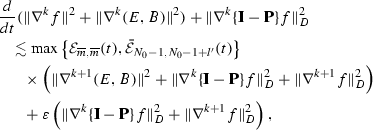
• (2) If $k=N_0-1$, it holds that

  $$\begin{aligned} \begin{aligned}&\frac{d}{dt}(\Vert \nabla ^{N_0-1}f\Vert ^2+\Vert \nabla ^{N_0-1}(E,B)\Vert ^2)+\Vert \nabla ^{N_0-1}\{\mathbf{I-P}\}f\Vert _D^2\\&\quad \lesssim \max \left\{ \mathcal {E}_{3,\frac{7}{2}+\frac{s-1}{\gamma }}(t),\mathcal {E}_{\overline{m},\overline{m}}(t),\mathcal {\bar{E}}_{N_0-1,N_0-1+l'}(t) \right\} \\&\qquad \times \big (\Vert \nabla ^{N_0-1}(E,B)\Vert ^2+\Vert \nabla ^{N_0-2}\{\mathbf{I-P}\}f\Vert _D^2+\Vert \nabla ^{N_0-1}f\Vert _D^2\big )+\varepsilon \Vert \nabla ^{N_0-1}f\Vert _D^2. \end{aligned} \end{aligned}$$

  (4.2)

• (3) For $k=N_0\ge 3$, if we take $n>\frac{2}{3}N_0-\frac{5}{3}$, one has

  $$\begin{aligned} \begin{aligned}&\frac{d}{dt}(\Vert \nabla ^{N_0}f\Vert ^2+\Vert \nabla ^{N_0}(E,B)\Vert ^2)+\Vert \nabla ^{N_0}\{\mathbf{I-P}\}f\Vert ^2_{D}\\&\quad \lesssim \max \left\{ \mathcal {E}_{N_0+n}(t),\mathcal {E}_{\overline{m},\overline{m}}(t), \mathcal {\bar{E}}_{N_0,N_0+l'}(t)\right\} \\&\qquad \times \left( \Vert \nabla ^{N_0-1}E\Vert ^2+\Vert \nabla ^{N_0-2}{\mathbf \{I-P\}}f\Vert _D^2+\Vert \nabla ^{N_0-1}f\Vert _D^2+\Vert \nabla ^{N_0}f\Vert _D^2\right) \\&\qquad +\varepsilon \left\{ \Vert \nabla ^{N_0-1}B\Vert ^2+\left\| \nabla ^{N_0-2}{\mathbf \{I-P\}}f\right\| ^2_{H^1_xL^2_D}+\left\| \nabla ^{N_0}f\right\| ^2_D\right\} . \end{aligned} \end{aligned}$$

  (4.3)

  Here $\overline{m}=\max \left\{ \frac{2\varrho +5}{2\varrho +3}N_0-\frac{6}{2\varrho +3},3+\frac{N_0-2+\varrho }{(\varrho +1)n+3-N_0}\right\}$ and $l'\ge \max \left\{ \frac{1}{2}+\frac{s-1}{\gamma },\frac{\hat{l}}{-\gamma }\right\}$ where $\hat{l}=\max \left\{ \hat{l}_1,\hat{l}_{2},\ldots ,\hat{l}_{19}\right\}$ where $\hat{l}_i$ will be specified in the proofs of Lemma 4.1.

Proof

For the case $k=0$, multiplying (1.4) by f and integrating the resulting identity with respect to x and v over $\mathbb {R}_x^3\times \mathbb {R}_v^3$, we have that

$$\begin{aligned} \begin{aligned} \frac{d}{dt}(\Vert f\Vert ^2+\Vert (E,B)\Vert ^2)+\Vert \{\mathbf{I-P}\}f\Vert ^2_{D}\lesssim |(v\cdot E f,f)|+|({\Gamma }(f,f),\{\mathbf{I-P}\}f)|, \end{aligned} \end{aligned}$$

(4.4)

For the first term on the right hand of (4.4), we have

$$\begin{aligned} \begin{aligned}&|(v\cdot E f,f)|\\&\quad \lesssim |(v\cdot E f,{\mathbf P}f)|+|(v\cdot E f,\{\mathbf{I-P}\}f)|\\&\quad \lesssim \Vert E\Vert _{L^2_x}\Vert \mu ^{\delta }f\Vert _{L^3_xL^2_v}\Vert \mu ^{\delta }f\Vert _{L^6_xL^2_v}+\Vert E\Vert _{L^6_x}\Vert \langle v\rangle ^{-\frac{\gamma }{2}-s+1}\{\mathbf{I-P}\}f\Vert _{L^3_xL^2_v}\\&\qquad \times \Vert \langle v\rangle ^{\frac{\gamma }{2}+s}\{\mathbf{I-P}\}f\Vert _{L^2_xL^2_v}\\&\quad \lesssim \Vert E\Vert \Vert \mu ^{\delta }f\Vert _{L^2_vL^3_x}\Vert \mu ^{\delta }f\Vert _{L^2_vL^6_x}+\Vert E\Vert _{L^2_vL^6_x}\Vert \langle v\rangle ^{-\frac{\gamma }{2}-s+1}\{\mathbf{I-P}\}f\Vert _{L^2_vL^3_x}\Vert \{\mathbf{I-P}\}f\Vert _D\\&\quad \lesssim \Vert \Lambda ^{-\frac{1}{2}}E\Vert ^{\frac{2}{3}}\Vert \nabla _xE\Vert ^{\frac{1}{3}}\Vert \Lambda ^{-\frac{1}{2}}f\Vert ^{\frac{1}{3}}\Vert \nabla _xf\Vert _D^{\frac{2}{3}}\Vert \nabla _xf\Vert _{D}+\Vert \nabla _xE\Vert \Vert \langle v\rangle ^{-\frac{\gamma }{2}-s+1}\{\mathbf{I-P}\}f\Vert _{H^1_x}\\&\qquad \times \Vert \{\mathbf{I-P}\}f\Vert _D\\&\quad \lesssim \mathcal {\bar{E}}_{1,\frac{3}{2}+\frac{s-1}{\gamma }}(t)(\Vert \nabla _xE\Vert ^2+\Vert \nabla _xf\Vert ^2_{D})+\varepsilon (\Vert \nabla _xf\Vert ^2_{D}+\Vert \{\mathbf{I-P}\}f\Vert ^2_{D}). \end{aligned} \end{aligned}$$

The other term can be estimated as follows

$$\begin{aligned} \begin{aligned}&|({\mathbf \Gamma }(f,f),\{\mathbf{I-P}\}f)|\\&\quad \lesssim \varepsilon \Vert \{\mathbf{I-P}\}f\Vert ^2_{D}+\Vert | f|_{L^2_{\gamma /2+s}}|f|_{L^2_D}\Vert ^2+\Vert | f|_{L^2_v}|f|_{L^2_{\gamma /2+s}}\Vert ^2\\&\quad \lesssim \varepsilon \Vert \{\mathbf{I-P}\}f\Vert ^2_{D}+\Vert f\Vert ^2_{L^3_x}\Vert f\Vert ^2_{L^6_xL^2_D} \,\lesssim \,\varepsilon \Vert \{\mathbf{I-P}\}f\Vert ^2_{D}+\Vert f\Vert ^2_{H^1_x}\Vert \nabla _xf\Vert ^2_D.\\ \end{aligned} \end{aligned}$$

Collecting the above estimates gives

$$\begin{aligned} \begin{aligned} \frac{d}{dt}(\Vert f\Vert ^2+\Vert (E,B)\Vert ^2)+\Vert \{\mathbf{I-P}\}f\Vert ^2_{D}\,\lesssim \,\mathcal {\bar{E}}_{1,\frac{3}{2}+\frac{s-1}{\gamma }}(t)(\Vert \nabla _xE\Vert ^2+\Vert \nabla _xf\Vert ^2_{D})+\varepsilon \Vert \nabla _xf\Vert ^2_{D} \end{aligned} \end{aligned}$$

(4.5)

which gives (4.1) with $k=0$.

For $k=1,2,\ldots ,N_0-2$, applying $\nabla ^k$ to (1.4), multiplying the resulting identity by $\nabla ^kf$, and then integrating the final result with respect to x and v over $\mathbb {R}_x^3\times \mathbb {R}_v^3$, we have that

$$\begin{aligned} \begin{aligned}&\frac{d}{dt}\left( \left\| \nabla ^kf\right\| ^2+\left\| \nabla ^k(E,B)\right\| ^2\right) +\left\| \nabla ^k\{\mathbf{I-P}\}f\right\| ^2_{\sigma }\\&\quad \lesssim \underbrace{\left| \left( \nabla ^k(v\cdot Ef),\nabla ^kf\right) \right| }_{I_1} +\underbrace{\left| \left( \nabla ^k(E\cdot \nabla _vf),\nabla ^kf\right) \right| }_{I_2}\\&\quad +\underbrace{\left| \left( \nabla ^k(v\times B\cdot \nabla _vf),\nabla ^kf\right) \right| }_{I_3}+\underbrace{\left| \left( \nabla ^k{\varvec{\Gamma }}(f,f),\nabla ^kf\right) \right| }_{I_4}. \end{aligned} \end{aligned}$$

(4.6)

By applying the macro-micro decomposition, one can deduce that

(4.7)

Applying Lemma 2.5, $I_{1,1}$ and $I_{1,2}$ can be dominated by

$$\begin{aligned} \begin{aligned} I_{1,1}+I_{1,2}&\lesssim \sum _{j\le k-1}\left\| \nabla ^jE\right\| _{L^6_x} \left\| \nabla ^{k-1-j}\left( \mu ^{\delta }f\right) \right\| _{L^3_xL^2_v}\left\| \nabla ^{k+1}\left( \mu ^{\delta }f\right) \right\| \\&\lesssim \sum _{j\le k-1}\left\| \Lambda ^{-\frac{1}{2}}E\right\| ^{\frac{2k-2j}{2k+3}} \left\| \nabla ^{k+1}E\right\| ^{\frac{2j+3}{2k+3}} \left\| \Lambda ^{-\frac{1}{2}}\left( \mu ^{\delta }f\right) \right\| ^{\frac{2j+3}{2k+3}} \left\| \nabla ^{k+1}\left( \mu ^{\delta }f\right) \right\| ^{\frac{2k-2j}{2k+3}}\\&\quad \times \left\| \nabla ^{k+1}\left( \mu ^{\delta }f\right) \right\| \\&\lesssim \mathcal {\bar{E}}_{0,0}(t)\left( \left\| \nabla ^{k+1}E\right\| ^2+\left\| \nabla ^{k+1}f\right\| _D^2\right) +\varepsilon \left\| \nabla ^{k+1}f\right\| _D^2. \end{aligned} \end{aligned}$$

For $I_{1,3}$, it holds from the Cauchy inequality and Holder inequalities that

$$\begin{aligned} \begin{aligned} I_{1,3} \lesssim&\sum _{j\le k}\left\| \nabla ^jE \nabla ^{k-j}\{\mathbf{I-P}\}f\langle v\rangle ^{1-\frac{\gamma +2s}{2}}\right\| \left\| \nabla ^k\{\mathbf{I-P}\}f\langle v\rangle ^{\frac{\gamma +2s}{2}}\right\| \\ \lesssim&\underbrace{\sum _{j\le k}\left\| \nabla ^jE \nabla ^{k-j}\{\mathbf{I-P}\}f\langle v\rangle ^{1-\frac{\gamma +2s}{2}}\right\| ^2}_{I_{1,3,1}}+\varepsilon \left\| \nabla ^k\{\mathbf{I-P}\}f\right\| ^2_D. \end{aligned} \end{aligned}$$

To deal with $I_{1,3,1}$, when $j=0$, we have from Lemma 2.5 that

$$\begin{aligned} \begin{aligned} I_{1,3,1}&\lesssim \left( \Vert E\Vert _{L^\infty _x}\left\| \nabla ^{k}\{\mathbf{I-P}\}f\langle v\rangle ^{1-\frac{\gamma +2s}{2}}\right\| \right) ^2\\&\lesssim \left( \left\| \Lambda ^{-\varrho }E\right\| ^{1-\theta }\left\| \nabla ^{k+1}E\right\| ^{\theta } \left\| \nabla ^{k}\{\mathbf{I-P}\}f\langle v\rangle ^{\frac{\gamma +2s}{2}}\right\| ^{1-\theta } \left\| \nabla ^{k}\{\mathbf{I-P}\}f\langle v\rangle ^{\hat{l}_1}\right\| ^{\theta }\right) ^2\\&\lesssim \, \mathcal {\bar{E}}_{k,k-\frac{\hat{l}_1}{\gamma }}(t)\left( \left\| \nabla ^{k+1}E\right\| ^2 +\left\| \nabla ^{k}\{\mathbf{I-P}\}f\right\| ^2_D\right) . \end{aligned} \end{aligned}$$

Here $\theta =\frac{3+2\varrho }{2(k+1+\varrho )}$ and $\hat{l}_1=\frac{1-\gamma -2s}{\theta }+\frac{\gamma +2s}{2}=\frac{2(1-\gamma -2s)(k+1+\varrho )}{3+2\varrho }+\frac{\gamma +2s}{2}.$

While for the case $j\ne 0$, we can deduce from Lemma 2.5 that

$$\begin{aligned} \begin{aligned} I_{1,3,1}&\lesssim \sum _{1\le j\le k}\left( \left\| \nabla ^jE\right\| _{L^6_x}\left\| \nabla ^{k-j}\{\mathbf{I-P}\}f\langle v\rangle ^{1-\frac{\gamma +2s}{2}}\right\| _{L^2_vL^3_x}\right) ^2\\&\lesssim \sum _{1\le j\le k}\left( \left\| \Lambda ^{-\varrho }E\right\| ^{1-\theta _j}\left\| \nabla ^{k+1}E\right\| ^{\theta _j} \left\| \{\mathbf{I-P}\}f\langle v\rangle ^{1-\frac{\gamma +2s}{2}}\right\| ^{1-\alpha _j}\right. \\&\quad \times \left. \left\| \nabla ^{k}\{\mathbf{I-P}\}f\langle v\rangle ^{1-\frac{\gamma +2s}{2}}\right\| ^{\alpha _j} \right) ^2\\&\lesssim \sum _{1\le j\le k}\left( \left\| \Lambda ^{-\varrho }E\right\| ^{1-\theta _j}\left\| \nabla ^{k+1}E\right\| ^{\theta _j} \left\| \{\mathbf{I-P}\}f\langle v\rangle ^{1-\frac{\gamma +2s}{2}}\right\| ^{1-\alpha _j}\right. \\&\quad \times \left. \left( \left\| \nabla ^{k}\{\mathbf{I-P}\}f\langle v\rangle ^{\hat{l}_{2j}}\right\| ^{1-\beta _j}\left\| \nabla ^{k}\{\mathbf{I-P}\}f\langle v\rangle ^{\frac{\gamma +2s}{2}}\right\| ^{\beta _j}\right) ^{\alpha _j}\right) ^2\\&\lesssim \sum _{1\le j\le k}\left( \left\| \Lambda ^{-\varrho }E\right\| ^{1-\theta _j} \left\| \{\mathbf{I-P}\}f\langle v\rangle ^{1-\frac{\gamma +2s}{2}}\right\| ^{1-\alpha _j}\left\| \nabla ^{k}\{\mathbf{I-P}\}f\langle v\rangle ^{\hat{l}_{2j}}\right\| ^{\alpha _j(1-\beta _j)}\right. \\&\quad \left. \times \left\| \nabla ^{k}\{\mathbf{I-P}\}f\langle v\rangle ^{\frac{\gamma +2s}{2}}\right\| ^{{\alpha _j}\beta _j}\left\| \nabla ^{k+1}E\right\| ^{\theta _j}\right) ^2\\&\lesssim \mathcal {\bar{E}}_{k,k-\frac{\hat{l}_{2}}{\gamma }}(t)\left( \left\| \nabla ^{k+1}E\right\| ^2+\left\| \nabla ^{k}\{\mathbf{I-P}\}f\right\| ^2_D\right) . \end{aligned} \end{aligned}$$

Here we can deduce from Lemma 2.5 that $\theta _j=\frac{j+\varrho +1}{k+1+\varrho },\ \alpha _j=\frac{2k-2j+1}{2k},\ \frac{\gamma +2s}{2}\cdot \beta _j+\hat{l}_{2j}(1-\beta _j)=1-\frac{\gamma +2s}{2}.$ If we set $\alpha _j\beta _j=1-\theta _j$, then we can get that $\hat{l}_{2j}=\frac{\gamma +2s}{2}+\frac{1-\gamma -2s}{1-\beta _j}=\frac{\gamma +2s}{2}+\frac{(1-\gamma -2s)(2k-2j+1)(k+1+\varrho )}{(2k-2j+1)(k+1+\varrho )-2k(k-j)}$ and we take $\hat{l}_2=\displaystyle \max \nolimits _{1\le j\le k}\left\{ \hat{l}_{2j}\right\}$.

Consequently

$$\begin{aligned} I_1\lesssim & {} \mathcal {\bar{E}}_{k,k-\frac{\max \{\hat{l}_1,\hat{l}_{2}\}}{\gamma }}(t)\left( \left\| \nabla ^{k+1}E\right\| ^2+\left\| \nabla ^{k+1}f\right\| _D^2 +\left\| \nabla ^{k} \{\mathbf{I-P}\}f\right\| ^2_D\right) + \varepsilon \left( \left\| \nabla ^{k+1}f\right\| _D^2\right. \\&\left. +\left\| \nabla ^k\{\mathbf{I-P}\}f\right\| ^2_D\right) . \end{aligned}$$

For $I_3$ on the right-hand side of (4.6), we can get

$$\begin{aligned} \begin{aligned} I_3\lesssim&\sum _{1\le j\le k}\left| \left( v\times \nabla ^{j}B\cdot \nabla _v\nabla ^{k-j}f,\nabla ^kf\right) \right| \\ =&\underbrace{ \sum _{1\le j\le k}\left| \left( v\times \nabla ^{j}B\cdot \nabla _v\nabla ^{k-j}{\mathbf P}f,\nabla ^kf\right) \right| }_{I_{3,1}}\\&+\underbrace{\sum _{1\le j\le k} \left| \left( v\times \nabla ^{j}B\cdot \nabla _v\nabla ^{k-j}\mathbf{\{I- P\}}f,\nabla ^k{\mathbf P}f\right) \right| }_{I_{3,2}}\\&+\underbrace{\sum _{1\le j\le k} \left| \left( v\times \nabla ^{j}B\cdot \nabla _v\nabla ^{k-j}\mathbf{\{I- P\}}f,\nabla ^k\mathbf{\{I- P\}}f\right) \right| }_{I_{3,3}}. \end{aligned} \end{aligned}$$

(4.8)

Applying the same trick as the estimate on $I_{1,1}$, $I_{3,1}$ and $I_{3,2}$ can be bounded by

$$\begin{aligned} \mathcal {\bar{E}}_{0,0}(t)\left( \left\| \nabla ^{k+1}B\right\| ^2+\left\| \nabla ^{k+1}f\right\| _D^2\right) +\varepsilon \left\| \nabla ^{k+1}f\right\| _D^2. \end{aligned}$$

For $I_{3,3}$, when $j=k$,

$$\begin{aligned} \begin{aligned} I_{3,3} \lesssim&\left\| \nabla ^{k}B\right\| _{L^6_x}\left\| \langle v\rangle ^{1-\frac{\gamma }{2}-s}\nabla _v\mathbf{\{I- P\}}f\right\| _{L^2_v L^3_x}\left\| \langle v\rangle ^{\frac{\gamma }{2}+s}\nabla ^k\mathbf{\{I- P\}}f\right\| _{L^2_vL^2_x} \\ \lesssim&\left\| \langle v\rangle ^{1-\frac{\gamma }{2}-s}\nabla _v\mathbf{\{I- P\}}f\right\| _{L^2_v L^3_x}\left\| \nabla ^{k+1}B\right\| \left\| \nabla ^{k}\mathbf{\{I- P\}}f\right\| _{D} \\ \lesssim&\,\mathcal {\bar{E}}_{2,\frac{5}{2}+\frac{s-1}{\gamma }}(t)\left\| \nabla ^{k+1}B\right\| ^2+\varepsilon \left\| \nabla ^k\{\mathbf{I-P}\}f\right\| ^2_{D}. \end{aligned} \end{aligned}$$

(4.9)

While for the case $1\le j\le k-1$,

$$\begin{aligned} \begin{aligned} I_{3,3} \lesssim&\sum _{1\le j\le k-1}\left\| \nabla ^{j}B\right\| _{L^\infty _x}\left\| \nabla _v\nabla ^{k-j}\mathbf{\{I- P\}}f\right\| \left\| \langle v\rangle \nabla ^k\mathbf{\{I- P\}}f\right\| \\ \lesssim&\sum _{1\le j\le k-1}\left\| \Lambda ^{-{\varrho }}B\right\| ^{\frac{2k-2j-1}{2(k+1+\varrho )}}\left\| \nabla ^{k+1}B\right\| ^{\frac{2j+2\varrho +3}{2(k+1+\varrho )}} \left\| \nabla ^{m_{1j}+1}_v\nabla ^{k-j}\mathbf{\{I- P\}}f\right\| ^{\frac{1}{m_{1j}+1}}\\&\times \left\| \nabla ^{k-j}\mathbf{\{I- P\}}f\right\| ^{\frac{m_{1j}}{m_{1j}+1}}\left\| \langle v\rangle \nabla ^k\mathbf{\{I- P\}}f\right\| \\ \lesssim&\sum _{1\le j\le k-1}\left\| \Lambda ^{-{\varrho }}B\right\| ^{\frac{2k-2j-1}{2(k+1+\varrho )}}\left\| \nabla ^{k+1}B\right\| ^{\frac{2j+2\varrho +3}{2(k+1+\varrho )}} \left\| \nabla ^{m_{1j}+1}_v\nabla ^{k-j}\mathbf{\{I- P\}}f\right\| ^{\frac{1}{m_{1j}+1}}\\&\times \left\| \Lambda ^{-{\varrho }}\mathbf{\{I- P\}}f\right\| ^{\frac{m_{1j}j}{(m_{1j}+1)(k+\varrho )}}\left\| \nabla ^{k}\mathbf{\{I- P\}}f\right\| ^{\frac{m_{1j}(k-j+\varrho )}{(m_{1j}+1)(k+\varrho )}}\left\| \langle v\rangle \nabla ^k\mathbf{\{I- P\}}f\right\| \\ \lesssim&\sum _{1\le j\le k-1}\left\| \Lambda ^{-{\varrho }}B\right\| ^{\frac{2k-2j-1}{2(k+1+\varrho )}}\left\| \nabla ^{k+1}B\right\| ^{\frac{2j+2\varrho +3}{2(k+1+\varrho )}} \left\| \nabla ^{m_{1j}+1}_v\nabla ^{k-j}\mathbf{\{I- P\}}f\right\| ^{\frac{1}{m_{1j}+1}}\\&\times \left\| \Lambda ^{-{\varrho }}\mathbf{\{I- P\}}f\right\| ^{\frac{m_{1j}j}{(m_{1j}+1)(k+\varrho )}}\left\| \langle v\rangle ^{\frac{\gamma +2s}{2}}\nabla ^{k}\mathbf{\{I- P\}}f\right\| ^{\frac{m_{1j}(k-j+\varrho )\beta _j}{(m_{1j}+1)(k+\varrho )}}\\&\times \left\| \langle v\rangle ^{\hat{l}_{3j}}\nabla ^{k}\mathbf{\{I- P\}}f\right\| ^{\frac{m_{1j}(k-j+\varrho )(1-\beta _j)}{(m_{1j}+1)(k+\varrho )}}\left\| \langle v\rangle ^{\frac{\gamma +2s}{2}}\nabla ^k\mathbf{\{I- P\}}f\right\| ^{\beta _j}\\&\times \left\| \langle v\rangle ^{\hat{l}_{4j}}\nabla ^k\mathbf{\{I- P\}}f\right\| ^{1-\beta _j} \\ \lesssim&\max \left\{ \mathcal {\bar{E}}_{k+m_{1},1+m_{1}}(t),\mathcal {\bar{E}}_{k,-\frac{\hat{l}_{4}}{\gamma }}(t)\right\} \left( \left\| \nabla ^{k+1}B\right\| ^2+\left\| \nabla ^k\{\mathbf{I-P}\}f\right\| ^2_{D}\right) \\&+\varepsilon \left\| \nabla ^k\{\mathbf{I-P}\}f\right\| ^2_{D}. \end{aligned} \end{aligned}$$

(4.10)

Here we have used the fact that there exists a positive constant $\beta _j\in (0,1)$ such that

$$\begin{aligned} \frac{2j+2\varrho +3}{2(k+1+\varrho )}+\frac{m_{1j}(k-j+\varrho )\beta _j}{(m_{1j}+1)(k+\varrho )}+\beta _j=2 \end{aligned}$$

holds for $1\le j\le k-1$. A necessary and sufficient condition to guarantee the existence of such a $\beta$ is

$$\begin{aligned} \frac{2j+2\varrho +3}{2(k+1+\varrho )}+\frac{m_{1j}(k-j+\varrho )}{(m_{1j}+1)(k+\varrho )}+1>2,\quad 1\le j\le k-1, \end{aligned}$$

from which one can deduce that $m_{1j}> \frac{2k^2+2\varrho k-2jk-k-2j\varrho -\varrho }{2k\varrho +3k+2\varrho ^2+3\varrho -2j}$ holds for $1\le j\le k-1$. Noticing that $\frac{1}{2}<\varrho <\frac{3}{2}$, it is easy to see that we can take

$$\begin{aligned} m_1=\max _{1\le j\le k-1}m_{1j}=\frac{2k}{2\varrho +3}+\frac{2\varrho -3}{2\varrho +3}>\frac{2k^2+2\varrho k-3k-3\varrho }{2k\varrho +3k+2\varrho ^2+3\varrho -2}. \end{aligned}$$

Consequently, $k-j+1+m_{1j}\le k+m_{1}=\frac{2\varrho +5}{2\varrho +3}k+\frac{2\varrho -3}{2\varrho +3}\le \frac{2\varrho +5}{2\varrho +3}N_0-\frac{2\varrho +13}{2\varrho +3}$ with $N_0\ge 4$.

Moreover, since $\hat{l}_{3j}$ and $\hat{l}_{4j}$ satisfy $\frac{\gamma +2s}{2}\beta _j+\hat{l}_{3j}(1-\beta _j)=0$ and $\frac{\gamma +2s}{2}{\beta _j}+\hat{l}_{4j}(1-\beta _j)=1$ with $0<\beta _j<1$ respectively, one can deduce that $\hat{l}_{3j}=\frac{\gamma +2s}{2}-\frac{\gamma +2s}{2(1-\beta _j)}$ and $\hat{l}_{4j}=\frac{\gamma +2s}{2}-\frac{\gamma +2s-2}{2(1-\beta _j)}$, from which we can see that $\hat{l}_{4j}>\hat{l}_{3j}$ where

$$\begin{aligned} \beta _j=\frac{(4k+1+2\varrho -2j)(m_{1j}+1)(k+\varrho )}{(k+2+2\varrho )(k+\varrho +2km_{1j}+2\varrho m_{1j}-jm_{1j})}. \end{aligned}$$

Here we take $\hat{l}_{4}=\displaystyle \max \nolimits _{1\le j\le k-1}\left\{ \hat{l}_{4j}\right\}$.

Consequently,

$$\begin{aligned} \begin{aligned} I_{3}&\lesssim \max \left\{ \mathcal {\bar{E}}_{k+m_{1},1+m_{1}}(t),\mathcal {\bar{E}}_{k,-\frac{\hat{l}_{4}}{\gamma }}(t),\mathcal {\bar{E}}_{2,\frac{5}{2}+\frac{s-1}{\gamma }}(t)\right\} \\&\quad \times \left( \left\| \nabla ^{k+1}B\right\| ^2 +\left\| \nabla ^k\{\mathbf{I-P}\}f\right\| ^2_{D}+\Vert \nabla ^{k+1}f\Vert _D^2\right) \\&\quad +\varepsilon \left( \Vert \nabla ^k\{\mathbf{I-P}\}f\Vert ^2_D+\Vert \nabla ^{k+1}f\Vert _D^2\right) . \end{aligned} \end{aligned}$$

By the same way as the estimate on $I_3$, the term $I_2$ containing E on the right-hand side of (4.6) can be bounded by

$$\begin{aligned} \begin{aligned} I_{2}&\lesssim \max \left\{ \mathcal {\bar{E}}_{k+m_{1},1+m_{1}}(t),\mathcal {\bar{E}}_{k,-\frac{\hat{l}_{4}}{\gamma }}(t),\mathcal {\bar{E}}_{2,\frac{5}{2}+\frac{s-1}{\gamma }}(t)\right\} \\&\quad \times \left( \left\| \nabla ^{k+1}E\right\| ^2 +\left\| \nabla ^k\{\mathbf{I-P}\}f\right\| ^2_{D}+\Vert \nabla ^{k+1}f\Vert _D^2\right) \\&\quad +\varepsilon \left( \Vert \nabla ^k\{\mathbf{I-P}\}f\Vert ^2_D+\Vert \nabla ^{k+1}f\Vert _D^2\right) . \end{aligned} \end{aligned}$$

For the last term $I_4$ on the right-hand side of (4.6), it follows that

$$\begin{aligned} \begin{aligned} I_4\lesssim&\sum _{j\le k}|({\Gamma }(\nabla ^{j}f,\nabla ^{k-j}f),\nabla ^k\{\mathbf{I-P}\}f)|\\ \lesssim&\sum _{j\le k}\int _{\mathbb {R}^3_x}\Big \{|\nabla ^jf|_{L^2_{\gamma +s/2}}|\nabla ^{k-j}f|_D+|\nabla ^{k-j}f|_{L^2_{\gamma +s/2}}|\nabla ^jf|_D\\&+\min \Big \{|\nabla ^jf|_{L^2}|\nabla ^{k-j}f|_{L^2_{\gamma +s/2}},|\nabla ^{k-j}f|_{L^2}|\nabla ^jf|_{L^2_{\gamma +s/2}}\Big \}\Big \}|\{\mathbf{I-P}\}f|_Ddx\\ \lesssim&\underbrace{\sum _{j\le k}\int _{\mathbb {R}^3_x}|\nabla ^j{\mathbf P}f|_{L^2}|\nabla ^{k-j}f|_D|\{\mathbf{I-P}\}f|_Ddx}_{I_{4,1}}\\&+\underbrace{\sum _{j\le k}\int _{\mathbb {R}^3_x}|\nabla ^j\{\mathbf{I-P}\}f|_{L^2}|\nabla ^{k-j}f|_D|\{\mathbf{I-P}\}f|_Ddx}_{I_{4,2}}\\ \end{aligned} \end{aligned}$$

(4.11)

The first term $I_{4,1}$ on the right-hand side of (4.11) can be estimated as follows:

$$\begin{aligned} \begin{aligned} I_{4,1} \lesssim&\sum _{j\le k}\Vert \nabla ^j {\mathbf P}f\Vert _{L^2_vL^6_x}\Vert \nabla ^{k-j}f\Vert _{L^2_D L^3_x}\Vert \nabla ^k\{\mathbf{I-P}\}f\Vert _D\\ \lesssim&\sum _{j\le k}\Vert \nabla ^{m'}{\mathbf P}f\Vert ^{1-\theta }\Vert \nabla ^{k+1} {\mathbf P}f\Vert ^{\theta }\Vert f\Vert _D^{\theta }\Vert \nabla ^{k+1}f\Vert _D^{1-\theta }\Vert \nabla ^k\{\mathbf{I-P}\}f\Vert _D\\ \lesssim&\max \left\{ \mathcal {E}_{N_0-1}(t),\mathcal {E}_{1,1}(t)\right\} \Vert \nabla ^{k+1} f\Vert _D^2+\varepsilon \Vert \nabla ^k\{\mathbf{I-P}\}f\Vert _D^2. \end{aligned} \end{aligned}$$

(4.12)

From Lemma 2.5, we can obtain

$$\begin{aligned} \theta =\frac{2j+1}{2(k+1)}, \quad m'=\frac{k+1}{2j+1}\le k+1\le N_0-1. \end{aligned}$$

When $j\le k-1$, the second term $I_{4,2}$ on the right-hand side of (4.11) can be bounded by

$$\begin{aligned} \begin{aligned} I_{4,2} \lesssim&\sum _{j\le k-1}\Vert \nabla ^j \{\mathbf{I- P}\}f\Vert _{L^2_vL^6_x}\Vert \nabla ^{k-j}f\Vert _{L^2_D L^3_x}\Vert \nabla ^k\{\mathbf{I-P}\}f\Vert _D\\ \lesssim&\sum _{j\le k-1}\Vert \{\mathbf{I- P}\}f\Vert ^{\frac{k-j-1}{k}}\Vert \nabla ^{k} \{\mathbf{I- P}\}f\Vert ^{\frac{j+1}{k}}\Vert f\Vert _D^{\frac{2j+1}{2(k+1)}}\Vert \nabla ^{k+1}f\Vert _D^{\frac{2k-2j}{2(k+1)}}\Vert \nabla ^k\{\mathbf{I-P}\}f\Vert _D\\ \lesssim&\sum _{j\le k-1}\Vert \{\mathbf{I- P}\}f\Vert ^{\frac{k-j-1}{k}}\Vert \nabla ^{k} \{\mathbf{I- P}\}f\langle v\rangle ^{\frac{\gamma }{2}+s}\Vert ^{\frac{j+1}{k}\beta }\Vert \nabla ^{k} \{\mathbf{I- P}\}f\langle v\rangle ^{\hat{l}_{5j}}\Vert ^{\frac{j+1}{k}(1-\beta )}\\&\times \Vert f\Vert _D^{\frac{2j+1}{2(k+1)}}\Vert \nabla ^{k+1}f\Vert _D^{\frac{2k-2j}{2(k+1)}}\Vert \nabla ^k\{\mathbf{I-P}\}f\Vert _D\\ \lesssim&\max \left\{ \mathcal {E}_{N_0-1,N_0-1-\frac{\hat{l}_{5}}{\gamma }}(t),\mathcal {E}_{1,1}(t)\right\} \Vert \nabla ^{k+1} f\Vert _D^2+\varepsilon \Vert \nabla ^k\{\mathbf{I-P}\}f\Vert _D^2. \end{aligned} \end{aligned}$$

(4.13)

Here $\frac{\gamma +2s}{2}\cdot \beta _j+\hat{l}_{5j}(1-\beta _j)=0.$ If we set $\frac{j+1}{k}\beta _j=\frac{2j+1}{2(k+1)}$, then we can get that $\hat{l}_{5j}=\frac{\gamma +2s}{2}+\frac{-\gamma -2s}{2(1-\beta _j)}=\frac{\gamma +2s}{2}+\frac{(-\gamma -2s)(k+1)(j+1)}{2(k+1)(j+1)-k(2j+1)}$ and we take $\hat{l}_{5}=\displaystyle \max \nolimits _{j\le k-1}\hat{l}_{5j}$.

When $j=k$,

$$\begin{aligned} \begin{aligned} I_{4,2} \lesssim&\sum _{j= k}\Vert \nabla ^k \{\mathbf{I- P}\}f\Vert _{L^2_vL^2_x}\Vert f\Vert _{L^2_D L^\infty _x}\Vert \nabla ^k\{\mathbf{I-P}\}f\Vert _D\\ \lesssim&\sum _{j= k}\Vert \nabla ^{k} \{\mathbf{I- P}\}f\langle v\rangle ^{\frac{\gamma }{2}+s}\Vert ^{\theta }\Vert \nabla ^{k} \{\mathbf{I- P}\}f\langle v\rangle ^{\hat{l}_6}\Vert ^{1-\theta }\Vert f\Vert _D^{\theta }\Vert \nabla ^{k+1}f\Vert _D^{1-\theta }\Vert \nabla ^k\{\mathbf{I-P}\}f\Vert _D\\ \lesssim&\max \left\{ \mathcal {E}_{N_0-1,N_0-1-\frac{\hat{l}_6}{\gamma }}(t),\mathcal {E}_{1,1}(t)\right\} \left( \Vert \nabla ^{k+1} f\Vert _D^2+\Vert \nabla ^k \{\mathbf{I- P}\}f\Vert _D^2\right) +\varepsilon \Vert \nabla ^k\{\mathbf{I-P}\}f\Vert _D^2. \end{aligned} \end{aligned}$$

Here $\theta =\frac{2k-1}{2(k+1)},$ $\frac{\gamma +2s}{2}\cdot \theta +\hat{l}_6(1-\theta )=0$ from Lemma 2.5 which deduce that $\hat{l}_6=-\frac{(2k-1)(\gamma +2s)}{6}$.

Consequently,

$$\begin{aligned} I_4\lesssim & {} \max \left\{ \mathcal {E}_{N_0-1,N_0-1-\frac{\max \{\hat{l}_5,\hat{l}_6\}}{\gamma }}(t),\mathcal {E}_{1,1}(t)\right\} \left( \Vert \nabla ^{k+1} f\Vert _D^2+\Vert \nabla ^k \{\mathbf{I- P}\}f\Vert _D^2\right) \nonumber \\&+\,\varepsilon \Vert \nabla ^k\{\mathbf{I-P}\}f\Vert _D^2. \end{aligned}$$

(4.14)

Collecting the above estimate gives (4.1). When $k=N_0-1\ge 2$, (4.6) tells us that

$$\begin{aligned} \begin{aligned}&\frac{d}{dt}\left( \left\| \nabla ^{N_0-1}f\right\| ^2+\left\| \nabla ^{N_0-1}(E,B)\right\| ^2\right) +\left\| \nabla ^{N_0-1}\{\mathbf{I-P}\}f\right\| ^2_{\sigma }\\&\quad \lesssim \underbrace{\left| \left( \nabla ^{N_0-1}(E\cdot vf),\nabla ^{N_0-1}f\right) \right| }_{I_5} +\underbrace{\left| \left( \nabla ^{N_0-1}(E\cdot \nabla _vf),\nabla ^{N_0-1}f\right) \right| }_{I_{6}}\\&\qquad +\underbrace{\left| \left( \nabla ^{N_0-1}(v\times B\cdot \nabla _vf),\nabla ^{N_0-1}f\right) \right| }_{I_{7}}+\underbrace{\left| \left( \nabla ^{N_0-1}{\Gamma }(f,f),\nabla ^{N_0-1}f\right) \right| }_{I_{8}}. \end{aligned} \end{aligned}$$

(4.15)

To estimate $I_5$, due to

$$\begin{aligned} \begin{aligned} I_5&\lesssim \underbrace{\left| \left( E\cdot v\nabla ^{N_0-1}f,\nabla ^{N_0-1}f\right) \right| }_{I_{5,1}} +\underbrace{\left| \left( \nabla ^{N_0-1} E\cdot vf,\nabla ^{N_0-1}f\right) \right| }_{I_{5,2}}\\&\quad +\underbrace{\sum _{1\le j\le N_0-2}\left| \left( \nabla ^{j} E\cdot v\nabla ^{N_0-1-j}f,\nabla ^{N_0-1}f\right) \right| }_{I_{5,3}}, \end{aligned} \end{aligned}$$

(4.16)

From Lemma 2.5, using $L^\infty -L^2-L^2$ Soblev inequality implies that

$$\begin{aligned} \begin{aligned} I_{5,1}&\lesssim \Vert E\Vert _{L^\infty _x}\left\| \nabla ^{N_0-1}f\langle v\rangle ^{1-\frac{\gamma +2s}{2}}\right\| \left\| \nabla ^{N_0-1}f\right\| _D\\&\lesssim \left\| \Lambda ^{-\varrho }E\right\| ^{1-\theta }\left\| \nabla ^{N_0-1}E\right\| ^{\theta }\left\| \nabla ^{N_0-1}f\langle v\rangle ^{\hat{l}_7}\right\| ^{\theta }\left\| \nabla ^{N_0-1}f\langle v\rangle ^{\frac{\gamma +2s}{2}}\right\| ^{1-\theta }\left\| \nabla ^{N_0-1}f\right\| _D\\&\lesssim \mathcal {\bar{E}}_{N_0-1,N_0-1-\frac{\hat{l}_7}{\gamma }}(t)\left( \left\| \nabla ^{N_0-1}E\right\| ^2+\left\| \nabla ^{N_0-1}f\right\| _D^2\right) +\varepsilon \left\| \nabla ^{N_0-1}f\right\| _D^2, \end{aligned} \end{aligned}$$

where $\theta =\frac{3+2\varrho }{2(N_0-1+\varrho )}$ and $\hat{l}_7=\frac{\gamma +2s}{2}+\frac{1-\gamma -2s}{\theta }=\frac{\gamma +2s}{2}+\frac{2(N_0-1+\varrho )(1-\gamma -2s)}{3+2\varrho },$

$$\begin{aligned} \begin{aligned} I_{5,2}\,\lesssim&\,\Vert \nabla ^{N_0-1} E\Vert \Vert f\langle v\rangle ^{-\gamma /2-s+1}\Vert _{L^\infty _x}\Vert \nabla ^{N_0-1}f\Vert _D\\ \lesssim&\,\,\mathcal {E}_{2,\frac{5}{2}+\frac{s-1}{\gamma }}(t)\Vert \nabla ^{N_0-1}E\Vert ^2+\varepsilon \Vert \nabla ^{N_0-1}f\Vert _D^2. \end{aligned} \end{aligned}$$

Applying $L^6-L^3-L^2$ Soblev inequality yields that

$$\begin{aligned} \begin{aligned} I_{5,3}&\lesssim \sum _{1\le j\le N_0-2}\Vert \nabla ^{j} E\Vert _{L^6_x}\Vert \nabla ^{N_0-1-j} f\langle v\rangle ^{-\gamma /2-s+1}\Vert _{L^3_x}\Vert \nabla ^{N_0-1}f\Vert _{D}\\&\lesssim \sum _{1\le j\le N_0-2}\Vert \Lambda ^{-\varrho }E\Vert ^{1-\theta _j}\Vert \nabla ^{N_0-1}E\Vert ^{\theta _j}\Vert \nabla ^{N_0-1}f\langle v\rangle ^{-\gamma /2-s+1}\Vert ^{\alpha _j}\Vert f\langle v\rangle ^{-\gamma /2-s+1}\Vert ^{1-\alpha _j}\\&\quad \times \Vert \nabla ^{N_0-1}f\Vert _D\\&\lesssim \sum _{1\le j\le N_0-2}\Vert \Lambda ^{-\varrho }E\Vert ^{1-\theta _j}\Vert \nabla ^{N_0-1}E\Vert ^{\theta _j}[\Vert \nabla ^{N_0-1}f\langle v\rangle ^{\hat{l}_{8j}}\Vert ^{1-\beta _j}\Vert \nabla ^{N_0-1}f\langle v\rangle ^{\frac{\gamma }{2}+s}\Vert ^{\beta _j}]^{\alpha _j}\\&\quad \times \Vert f\langle v\rangle ^{-\gamma /2-s+1}\Vert ^{1-\alpha _j}\Vert \nabla ^{N_0-1}f\Vert _D\\&\lesssim \sum _{1\le j\le N_0-2}\Vert \Lambda ^{-\varrho }E\Vert ^{1-\theta _j}\Vert f\langle v\rangle ^{-\gamma /2}\Vert ^{1-\alpha _j}\Vert \nabla ^{N_0-1}f\langle v\rangle ^{\hat{l}_{8j}}\Vert ^{\alpha _j-\alpha _j\beta _j}\Vert \nabla ^{N_0-1}E\Vert ^{\theta _j}\\&\quad \times \Vert \nabla ^{N_0-1}f\langle v\rangle ^{\frac{\gamma }{2}+s}\Vert ^{\alpha _j\beta _j}\Vert \nabla ^{N_0-1}f\Vert _D\\&\lesssim \mathcal {\bar{E}}_{N_0-1,N_0-1-\frac{\hat{l}_{8}}{\gamma }}(t)\left( \Vert \nabla ^{N_0-1}E\Vert ^2+\Vert \nabla ^{N_0-1}f\Vert _D^2\right) +\varepsilon \Vert \nabla ^{N_0-1}f\Vert _D^2.\\ \end{aligned} \end{aligned}$$

(4.17)

Here $\theta _j=\frac{j+\varrho +1}{N_0-1+\varrho }$ and $\alpha _j=\frac{2N_0-1-j}{2(N_0-1)}$ by using Lemma 2.5. Meanwhile, we set $\alpha _j\beta _j=1-\theta _j$ and $\hat{l}_{8j}$ satisfies

$$\begin{aligned} \frac{\gamma +2s}{2}\cdot \beta _j+\hat{l}_{8j}(1-\beta _j)=-\frac{\gamma }{2}-s+1, \end{aligned}$$

it is easy to obtain that $\hat{l}_{8j}=\frac{1-\gamma -2s}{1-\beta _j}+\frac{\gamma +2s}{2}$ where $\beta _j=\frac{2(N_0-j-2)(N_0-1)}{(N_0-1+\varrho )(2N_0-1-j)}$. We take $\hat{l}_{8}=\displaystyle \max \nolimits _{1\le j\le N_0-2}\left\{ \hat{l}_{8j}\right\}$.

Consequently,

$$\begin{aligned} I_5\lesssim & {} \max \left\{ \mathcal {E}_{2,\frac{5}{2}+\frac{s-1}{\gamma }}(t),\mathcal {\bar{E}}_{N_0-1,N_0-1-\frac{\max \{\hat{l}_{7},\hat{l}_{8}\}}{\gamma }}(t)\right\} \left( \Vert \nabla ^{N_0-1}E\Vert ^2+\Vert \nabla ^{N_0-1}f\Vert _D^2\right) \nonumber \\&+\,\varepsilon \Vert \nabla ^{N_0-1}f\Vert _D^2 \end{aligned}$$

(4.18)

The third term $I_{7}$ on the right-hand side of (4.15) can be estimated as follows:

$$\begin{aligned} \begin{aligned} I_{7}\lesssim&\underbrace{|(v\times \nabla ^{N_0-1}B\cdot \nabla _vf,\nabla ^{N_0-1}f)|}_{I_{7,1}}+\underbrace{|(v\times \nabla ^{N_0-2} B\cdot \nabla _x\nabla _vf,\nabla ^{N_0-1}f)|}_{I_{7,2}}\\&+\underbrace{\sum _{1\le j\le N_0-3}|(\nabla ^j E\cdot \nabla ^{N_0-1-j}\nabla _vf,\nabla ^{N_0-1}f)|}_{I_{7,3}}. \end{aligned} \end{aligned}$$

(4.19)

$I_{7,1}$ and $I_{7,2}$ on the right-hand side of (4.19) can be bounded by

$$\begin{aligned} \begin{aligned} I_{7,1}+I_{7,2} \lesssim&\,\left\| \nabla _v\nabla f\langle v\rangle ^{1-\gamma /2-s}\right\| _{H^1}\left\| \nabla ^{N_0-1}B\right\| \left\| \nabla ^{N_0-1}f\right\| _D\\ \lesssim&\;\mathcal {E}_{3,\frac{7}{2}+\frac{s-1}{\gamma }}(t)\left\| \nabla ^{N_0-1}B\right\| ^2+\varepsilon \left\| \nabla ^{N_0-1}f\right\| _D^2.\\ \end{aligned} \end{aligned}$$

(4.20)

$I_{7,3}$ on the right-hand side of (4.19) can be bounded by

$$\begin{aligned} \begin{aligned} I_{7,3}&\lesssim \sum _{1\le j\le N_0-3}\left| \left( v\times \nabla ^j B\cdot \nabla ^{N_0-1-j} \nabla _v{\mathbf P}f,\nabla ^{N_0-1}f\right) \right| \\&\quad +\sum _{1\le j\le N_0-3}\left| \left( v\times \nabla ^j B\cdot \nabla ^{N_0-1-j}\nabla _v\{\mathbf{I-P}\}f,\nabla ^{N_0-1}f\right) \right| \\&\lesssim \mathcal {\bar{E}}_{0,0}(t)\left( \left\| \nabla ^{N_0-1}B\right\| ^2+\left\| \nabla ^{N_0-1}f\right\| _D^2\right) +\varepsilon \left\| \nabla ^{N_0-1}f\right\| _D^2\\&\quad + \sum _{1\le j\le N_0-3}\left\| \Lambda ^{-{\varrho }}B\right\| ^{\frac{2N_0-2j-5}{2(N_0-1+\varrho )}}\left\| \nabla ^{N_0-1}B\right\| ^{\frac{2j+2\varrho +3}{2(N_0-1+\varrho )}} \left\| \nabla ^{m_{2j}+1}_v\nabla ^{N_0-1-j}\{\mathbf{I-P}\}f\right\| ^{\frac{1}{m_{2j}+1}} \\&\quad \times \left\| \nabla ^{N_0-1-j}\{\mathbf{I-P}\}f\right\| ^{\frac{m_{2j}}{m_{2j}+1}}\left\| \langle v\rangle \nabla ^{N_0-1}f\right\| \\&\lesssim \mathcal {\bar{E}}_{0,0}(t)\left( \left\| \nabla ^{N_0-1}B\right\| ^2+\left\| \nabla ^{N_0-1}f\right\| _D^2\right) +\varepsilon \left\| \nabla ^{N_0-1}f\right\| _D^2\\&\quad +\sum _{1\le j\le N_0-3}\left\| \Lambda ^{-{\varrho }}B\right\| ^{\frac{2N_0-2j-5}{2(N_0-1+\varrho )}}\left\| \nabla ^{N_0-1}B\right\| ^{\frac{2j+2\varrho +3}{2(N_0-1+\varrho )}} \left\| \nabla ^{m_{2j}+1}_v\nabla ^{N_0-1-j}\{\mathbf{I-P}\}f\right\| ^{\frac{1}{m_{2j}+1}}\\&\quad \times \left\| \Lambda ^{-\varrho }\{\mathbf{I-P}\}f\right\| ^{\frac{m_{2j}j}{(m_{2j}+1)(N_0-1+\varrho )}}\left\| \nabla ^{N_0-1}\{\mathbf{I-P}\}f\right\| ^{\frac{m_{2j}(N_0-1+\varrho -j)}{(m_{2j}+1)(N_0-1+\varrho )}}\left\| \langle v\rangle \nabla ^{N_0-1}f\right\| \\&\lesssim \mathcal {\bar{E}}_{0,0}(t)\left( \left\| \nabla ^{N_0-1}B\right\| ^2+\left\| \nabla ^{N_0-1}f\right\| _D^2\right) +\varepsilon \left\| \nabla ^{N_0-1}f\right\| _D^2\\&\quad +\sum _{1\le j\le N_0-3}\left\| \Lambda ^{-{s}}B\right\| ^{\frac{2N_0-2j-5}{2(N_0-1+\varrho )}}\left\| \nabla ^{N_0-1}B\right\| ^{\frac{2j+2\varrho +3}{2(N_0-1+\varrho )}} \left\| \nabla ^{m_{2j}+1}_v\nabla ^{N_0-1-j}\{\mathbf{I-P}\}f\right\| ^{\frac{1}{m_{2j}+1}}\\&\quad \times \left\| \Lambda ^{-\varrho }\{\mathbf{I-P}\}f\right\| ^{\frac{m_{2j}j}{(m_{2j}+1)(N_0-1+\varrho )}}\left\| \langle v\rangle ^{\hat{l}_{9j}}\nabla ^{N_0-1}\{\mathbf{I-P}\}f\right\| ^{\frac{m_{2j}(N_0-1+\varrho -j)(1-\beta _j)}{(m_{2j}+1)(N_0-1+\varrho )}}\\&\quad \times \left\| \langle v\rangle ^{\frac{\gamma +2s}{2}}\nabla ^{N_0-1}\{\mathbf{I-P}\}f\right\| ^{\frac{m_{2j}(N_0-1+\varrho -j)\beta _j}{(m_{2j}+1)(N_0-1+\varrho )}}\left\| \langle v\rangle ^{\hat{l}_{10j}}\nabla ^{N_0-1}f\right\| ^{1-\beta _j}\left\| \langle v\rangle ^{\frac{\gamma +2s}{2}}\nabla ^{N_0-1}f\right\| ^{\beta _j}\\&\lesssim \max \left\{ \mathcal {E}_{3,\frac{7}{2}+\frac{s-1}{\gamma }}(t),\mathcal {E}_{N_0-1+m_{2},m_{2}+1}(t),\mathcal {\bar{E}}_{N_0-1,N_0-1-\frac{\hat{l}_{10}}{\gamma }}(t) \right\} \\&\quad \times \left( \left\| \nabla ^{N_0-1}B\right\| ^2+\left\| \nabla ^{N_0-1}f\right\| _D^2\right) +\varepsilon \left\| \nabla ^{N_0-1}f\right\| _D^2. \end{aligned} \end{aligned}$$

(4.21)

Here we have used the fact that there exists a positive constant $\beta _j\in (0,1)$ such that

$$\begin{aligned} \frac{2j+2\varrho +3}{2(N_0-1+\varrho )}+\frac{m_{2j}(N_0-1+\varrho -j)\beta _j}{(m_{2j}+1)(N_0-1+\varrho )}+\beta _j=2 \end{aligned}$$

holds for $1\le j\le N_0-3$. A necessary and sufficient condition to guarantee the existence of such a $\beta$ is

$$\begin{aligned} \frac{2j+2\varrho +3}{2(N_0-1+\varrho )}+\frac{m_{2j}(N_0-1+\varrho -j)}{(m_{2j}+1)(N_0-1+\varrho )}+1>2,\quad 1\le j\le N_0-3, \end{aligned}$$

from which one can deduce that $m_{2j}>\frac{2N_0-5-2j}{2\varrho +3}$ holds for $1\le j\le N_0-3$. Noticing that $\frac{1}{2}<\varrho <\frac{3}{2}$, it is easy to see that we can take

$$\begin{aligned} m_2=\max _{1\le j\le k-1}m_{2j}=\frac{2N_0}{2\varrho +3}-\frac{6}{2\varrho +3}>\max _{1\le j\le k-1}\frac{2N_0-5-2j}{2\varrho +3}. \end{aligned}$$

Consequently, $N_0-j+m_{2j}\le N_0+m_{2}=\frac{2\varrho +5}{2\varrho +3}N_0-\frac{6}{2\varrho +3}$ with $N_0\ge 4$.

Moreover, since $\hat{l}_{9j}$ and $\hat{l}_{10j}$ satisfy $\frac{\gamma +2s}{2}\beta _j+\hat{l}_{9j}(1-\beta _j)=0$ and $\frac{\gamma +2s}{2}{\beta _j}+\hat{l}_{10j}(1-\beta _j)=1$ with $0<\beta _j<1$ respectively, one can deduce that $\hat{l}_{9j}=\frac{\gamma +2s}{2}-\frac{\gamma +2s}{2(1-\beta )}$ and $\hat{l}_{10j}=\frac{\gamma +2s}{2}-\frac{\gamma +2s-2}{2(1-\beta _j)}$, from which we can see that $\hat{l}_{10j}>\hat{l}_{9j}$ where

$$\begin{aligned} \beta _j=\frac{(m_{2j}+1)(4N_0+2\varrho -2j-7)}{2\left( N_0-1+\varrho +m_{2j}\left( 2N_0-2+2\varrho -j\right) \right) }. \end{aligned}$$

Here we take $\hat{l}_{10}=\displaystyle \max \nolimits _{1\le j\le N_0-3}\left\{ \hat{l}_{10j}\right\}$. Consequently,

$$\begin{aligned} I_7\lesssim & {} \max \left\{ \mathcal {E}_{N_0-1+m_{2},m_{2}+1}(t),\mathcal {\bar{E}}_{N_0,N_0-\frac{\hat{l}_{10}}{\gamma }}(t) \right\} \left( \left\| \nabla ^{N_0-1}E\right\| ^2+\left\| \nabla ^{N_0-1}f\right\| _D^2\right) \\&+\,\varepsilon \left\| \nabla ^{N_0-1}f\right\| _D^2. \end{aligned}$$

Applying the same trick as $I_7$ by replacing $v\times B$ with E, one can obtain

$$\begin{aligned} I_6\lesssim & {} \max \left\{ \mathcal {E}_{N_0-1+m_{2},m_{2}+1}(t),\mathcal {\bar{E}}_{N_0,N_0-\frac{\hat{l}_{10}}{\gamma }}(t) \right\} \left( \left\| \nabla ^{N_0-1}B\right\| ^2+\left\| \nabla ^{N_0-1}f\right\| _D^2\right) \\&+\,\varepsilon \left\| \nabla ^{N_0-1}f\right\| _D^2. \end{aligned}$$

For the last term $I_{8}$ on the right hand side of (4.15), as (4.11), one has

$$\begin{aligned} \begin{aligned} I_{8}&\lesssim |({\Gamma }(f,\nabla ^{N_0-1}f),\nabla ^{N_0-1}f)|+|({\Gamma }(\nabla ^{N_0-1}f,f),\nabla ^{N_0-1}f)|\\&\quad +|({\Gamma }(\nabla f,\nabla ^{N_0-2}f),\nabla ^{N_0-1}f)|+|({\Gamma }(\nabla ^{N_0-2}f,\nabla f),\nabla ^{N_0-1}f)|\\&\quad +\sum _{2\le j\le N_0-3}|({\Gamma }(\nabla ^j f,\nabla ^{N_0-1-j}f),\nabla ^{N_0-1}f)|\\&\lesssim \mathcal {E}_{N_0-1,N_0-1+l'}(t)\left( \Vert \nabla ^{N_0-2}\{\mathbf{I-P}\}f\Vert _D^2+\Vert \nabla ^{N_0-1}f\Vert _D^2\right) +\varepsilon \Vert \nabla ^{N_0-1}f\Vert _D^2. \end{aligned} \end{aligned}$$

(4.22)

Collecting the above estimates gives (4.2). Now we turn to the last case $k=N_0\ge 3$, we have

$$\begin{aligned} \begin{aligned}&\frac{d}{dt}(\Vert \nabla ^{N_0}f\Vert ^2+\Vert \nabla ^{N_0}(E,B)\Vert ^2)+\Vert \nabla ^{N_0}\{\mathbf{I-P}\}f\Vert ^2_{D}\\&\quad \lesssim \underbrace{\left| \left( \nabla ^{N_0}(E\cdot vf),\nabla ^{N_0}f\right) \right| }_{{I_{9}}}+\underbrace{\left| \left( \nabla ^{N_0}(E\cdot \nabla _vf),\nabla ^{N_0}f\right) \right| }_{I_{10}}\\&\qquad +\underbrace{\left| \left( \nabla ^{N_0}(v\times B\cdot \nabla _vf),\nabla ^{N_0}f\right) \right| }_{I_{11}}+\underbrace{\left| \left( \nabla ^{N_0}{\Gamma }(f,f),\nabla ^{N_0}f\right) \right| }_{I_{12}}. \end{aligned} \end{aligned}$$

(4.23)

For the first term $I_{9}$ on the right hand of the above inequality,

$$\begin{aligned} \begin{aligned} I_{9}&\lesssim \underbrace{|(E\cdot v\nabla ^{N_0}f,\nabla ^{N_0}f)|}_{I_{9,1}}+\underbrace{|(\nabla E\cdot v\nabla ^{N_0-1}f,\nabla ^{N_0}f)|}_{I_{9,2}} +\underbrace{|(\nabla ^{N_0-1} E\cdot v\nabla f,\nabla ^{N_0}f)|}_{I_{9,3}}\\&\quad +\underbrace{|(\nabla ^{N_0} E\cdot vf,\nabla ^{N_0}f)|}_{I_{9,4}}+\underbrace{\sum _{2\le j\le N_0-2}|(\nabla ^{j} E\cdot v\nabla ^{N_0-j}f,\nabla ^{N_0}f)|}_{I_{9,5}}. \end{aligned} \end{aligned}$$

(4.24)

$I_{9,1}$ and $I_{9,2}$ can be bounded by

$$\begin{aligned} \begin{aligned} I_{9,1}+I_{9,2}&\lesssim \Vert E\Vert _{L^\infty }\Vert \nabla ^{N_0}f\langle v\rangle ^{-\frac{\gamma }{2}-s+1}\Vert \Vert \nabla ^{N_0}f\Vert _D+\Vert \nabla E\Vert _{L^3}\Vert \nabla ^{N_0-1}f\langle v\rangle ^{-\frac{\gamma }{2}}\Vert _{L^6}\Vert \nabla ^{N_0}f\Vert _D\\&\lesssim \Vert \Lambda ^{-\varrho }E\Vert ^{1-\theta }\Vert \nabla ^{N_0-1}E\Vert ^{\theta }\Vert \nabla ^{N_0}f\langle v\rangle ^{\hat{l}_{11}}\Vert ^\theta \Vert \nabla ^{N_0}f\langle v\rangle ^{\frac{\gamma }{2}+s}\Vert ^{1-\theta }\Vert \nabla ^{N_0}f\Vert _D\\&\lesssim \mathcal {\bar{E}}_{N_0,N_0-\frac{\hat{l}_{11}}{\gamma }}(t)(\Vert \nabla ^{N_0-1}E\Vert ^2+\Vert \nabla ^{N_0}f\Vert _D^2)+\varepsilon \Vert \nabla ^{N_0}f\Vert _D^2. \end{aligned} \end{aligned}$$

Here we can deduce that $\theta =\frac{3+2\varrho }{2(N_0-1+\varrho )}$ from Lemma 2.5, and $\hat{l}_{11}$ satisfies the following equation $\hat{l}_{11}\theta +\frac{\gamma +2s}{2}(1-\theta )=-\frac{\gamma }{2}-s+1$ which deduces that $\hat{l}_{11}=\frac{\gamma +2s}{2}-\frac{\gamma +2s-1}{\theta }=\frac{\gamma +2s}{2}-\frac{2(N_0-1+\varrho )(\gamma +2s-1)}{3+2\varrho }$.

Using $L^2-L^\infty -L^2$ gives

$$\begin{aligned} \begin{aligned} I_{9,3}\lesssim&\, \Vert \nabla ^{N_0-1} E\Vert \Vert \nabla f\langle v\rangle ^{1-\frac{\gamma }{2}-s}\Vert _{L^\infty _x}\Vert \nabla ^{N_0}f\Vert _D\\ \lesssim&\,\mathcal {E}_{3,\frac{7}{2}-\frac{1-s}{\gamma }}(t)\Vert \nabla ^{N_0-1}E\Vert ^2+\varepsilon \Vert \nabla ^{N_0}f\Vert _D^2.\\ \end{aligned} \end{aligned}$$

Applying the similar method as (4.17), the last term $I_{9,5}$ on the right-hand side of (4.24) can be dominated by

$$\begin{aligned} \begin{aligned} I_{9,5}&\lesssim \sum _{2\le j\le N_0-2}\Vert \nabla ^{j} E\Vert _{L^6}\Vert \nabla ^{N_0-j}f\langle v\rangle ^{-\frac{\gamma }{2}-s+1}\Vert _{L^3}\Vert \nabla ^{N_0}f\Vert _{D}\\&\lesssim \sum _{2\le j\le N_0-2}\Vert \Lambda ^{-\varrho }E\Vert ^{1-\theta _j}\Vert \nabla ^{N_0-1}E\Vert ^{\theta _j}\Vert \nabla ^{N_0-1}f\langle v\rangle ^{-\frac{\gamma }{2}-s+1}\Vert ^{\alpha _j}\Vert f\langle v\rangle ^{-\frac{\gamma }{2}-s+1}\Vert ^{1-\alpha _j}\\&\quad \times \Vert \nabla ^{N_0}f\Vert _D\\&\lesssim \sum _{2\le j\le N_0-2}\Vert \Lambda ^{-\varrho }E\Vert ^{1-\theta _j}\Vert \nabla ^{N_0-1}E\Vert ^{\theta _j}[\Vert \nabla ^{N_0-1}f\langle v\rangle ^{\hat{l}_{12j}}\Vert ^{1-\beta _j}\Vert \nabla ^{N_0-1}f\langle v\rangle ^{\frac{\gamma }{2}+s}\Vert ^{\beta _j}]^{\alpha _j}\\&\quad \times \Vert f\langle v\rangle ^{-\frac{\gamma }{2}-s+1}\Vert ^{1-\alpha _j}\Vert \nabla ^{N_0}f\Vert _D\\&\lesssim \sum _{2\le j\le N_0-2}\Vert \Lambda ^{-\varrho }E\Vert ^{1-\theta _j}\Vert f\langle v\rangle ^{-\frac{\gamma }{2}-s+1}\Vert ^{1-\alpha _j}\Vert \nabla ^{N_0-1}f\langle v\rangle ^{\hat{l}_{12j}}\Vert ^{\alpha _j-\alpha _j\beta _j}\Vert \nabla ^{N_0-1}E\Vert ^{\theta _j}\\&\quad \times \Vert \nabla ^{N_0-1}f\langle v\rangle ^{\frac{\gamma }{2}+s}\Vert ^{\alpha _j\beta _j}\Vert \nabla ^{N_0}f\Vert _D\\&\lesssim \mathcal {\bar{E}}_{N_0-1,N_0-1-\frac{\hat{l}_{12}}{\gamma }}(t)(\Vert \nabla ^{N_0-1}E\Vert ^2+\Vert \nabla ^{N_0-1}f\Vert _D^2)+\varepsilon \Vert \nabla ^{N_0}f\Vert _D^2.\\ \end{aligned} \end{aligned}$$

(4.25)

Here $\theta _j=\frac{j+1+\varrho }{N_0-1+\varrho }$ and $\alpha _j=\frac{2N_0-2j+1}{2(N_0-1)}$ by using Lemma 2.5. Meanwhile, we set $\alpha _j\beta _j=1-\theta _j$ and $\hat{l}_{12j}$ satisfies

$$\begin{aligned} \frac{\gamma +2s}{2}\cdot \beta _j+\hat{l}_{12j}(1-\beta _j)=-\frac{\gamma }{2}-s+1, \end{aligned}$$

it is easy to obtain that $\hat{l}_{12j}=-\frac{\gamma +2s-1}{1-\beta _j}+\frac{\gamma +2s}{2}$ where $\beta _j=\frac{2(N_0-2-j)(N_0-1)}{(2N_0-2j+1)(N_0-1+\varrho )}$. Here we take $\hat{l}_{12}=\displaystyle \max \nolimits _{2\le j\le N_0-2}\hat{l}_{12j}$.

For the most important term $I_{9,4}$, if $n>\frac{2}{3}N_0-\frac{5}{3}$, we have from Lemma 2.5 that

$$\begin{aligned} \begin{aligned} I_{9,4}&\lesssim \Vert \nabla ^{N_0-1}E\Vert ^{\frac{n}{n+1}}\Vert \nabla ^{N_0+n}\Vert ^{\frac{1}{n+1}}\Vert \langle v\rangle ^{-\frac{\gamma }{2}-s+1}f\Vert ^\frac{2N_0-5}{2N_0-2}\Vert \langle v\rangle ^{-\frac{\gamma }{2}-s+1}\nabla ^{N_0-1}f\Vert ^{\frac{3}{2N_0-2}}\\&\quad \times \Vert \nabla ^{N_0}f\Vert _{D}\\&\lesssim \Vert \nabla ^{N_0-1}E\Vert ^{\frac{n}{n+1}}\Vert \nabla ^{N_0+n}\Vert ^{\frac{1}{n+1}}\big [\Vert \langle v\rangle ^{\hat{l}_{13}}\nabla ^{N_0-1}f\Vert ^{1-\alpha }\Vert \langle v\rangle ^{\frac{\gamma +2s}{2}}\nabla ^{N_0-1}f\Vert ^{\alpha }\big ]^{\frac{3}{2N_0-2}}\\&\quad \times \Vert \langle v\rangle ^{-\frac{\gamma }{2}-s+1}f\Vert ^\frac{2N_0-5}{2N_0-2}\Vert \nabla ^{N_0}f\Vert _{D}\\&\lesssim \Vert \nabla ^{N_0-1}E\Vert ^{\frac{n}{n+1}}\Vert \nabla ^{N_0+n}\Vert ^{\frac{1}{n+1}}\Vert \langle v\rangle ^{\frac{\gamma +2s}{2}}\nabla ^{N_0-1}f\Vert ^{\frac{3\alpha }{2N_0-2}}\Vert \langle v\rangle ^{\hat{l}_{13}}\nabla ^{N_0-1}f\Vert ^{\frac{3(1-\alpha )}{2N_0-2}}\\&\quad \times \Vert \langle v\rangle ^{-\frac{\gamma }{2}-s+1}f\Vert ^\frac{2N_0-5}{2N_0-2}\Vert \nabla ^{N_0}f\Vert _{D}\\&\lesssim \Vert \nabla ^{N_0-1}E\Vert ^{\frac{n}{n+1}}\Vert \nabla ^{N_0+n}\Vert ^{\frac{1}{n+1}}\Vert \langle v\rangle ^{\frac{\gamma +2s}{2}}\nabla ^{N_0-1}f\Vert ^{\frac{3\alpha }{2N_0-2}}\Vert \langle v\rangle ^{\hat{l}_{13}}\nabla ^{N_0-1}f\Vert ^{\frac{3(1-\alpha )}{2N_0-2}}\\&\quad \times \Vert \langle v\rangle ^{-\frac{\gamma }{2}-s+1}f\Vert ^\frac{2N_0-5}{2N_0-2}\Vert \nabla ^{N_0}f\Vert _{D}\\&\lesssim \Vert \nabla ^{N_0-1}E\Vert ^{\frac{n}{n+1}}\Vert \nabla ^{N_0+n}\Vert ^{\frac{1}{n+1}}\Vert \langle v\rangle ^{\frac{\gamma +2s}{2}}\nabla ^{N_0-1}f\Vert ^{\frac{1}{n+1}}\Vert \langle v\rangle ^{\hat{l}_{13}}\nabla ^{N_0-1}f\Vert ^{\frac{3(1-\alpha )}{2N_0-2}}\\&\quad \times \Vert \langle v\rangle ^{-\frac{\gamma }{2}-s+1}f\Vert ^\frac{2N_0-5}{2N_0-2}\Vert \nabla ^{N_0}f\Vert _{D}\\&\lesssim \max \{\mathcal {E}_{N_0+n}(t),\mathcal {\bar{E}}_{N_0-1,N_0-1-\frac{\hat{l}_{13}}{\gamma }}(t)\}\left( \Vert \nabla ^{N_0-1}E\Vert ^2+\Vert \nabla ^{N_0-1}f\Vert _D^2\right) +\varepsilon \Vert \nabla ^{N_0}f\Vert _D^2. \end{aligned} \end{aligned}$$

(4.26)

Here we require that $\frac{3\alpha }{2N_0-2}=\frac{1}{n+1}$ which deduces that $\alpha =\frac{2N_0-2}{3(n+1)}$. We set $\frac{\gamma +2s}{2}\cdot \alpha +\hat{l}_{13}(1-\alpha )=1-\frac{\gamma }{2}-s$ which yields that $\hat{l}_{13}=\frac{1-\frac{\gamma }{2}-s-\frac{\gamma +2s}{2}\cdot \alpha }{1-\alpha }=\frac{\gamma +2s}{2}+\frac{1-\gamma -2s}{1-\alpha }=\frac{\gamma +2s}{2}+\frac{3(1-\gamma -2s)(n+1)}{3n-2 N_0+1}.$

Consequently, one has

$$\begin{aligned} I_{9}\lesssim & {} \max \left\{ \mathcal {E}_{3,\frac{7}{2}-\frac{1-s}{\gamma }}(t),\mathcal {E}_{N_0+n}(t),\mathcal {\bar{E}}_{N_0-1,N_0-\frac{\max \{\hat{l}_{11},\hat{l}_{12},\hat{l}_{13}\}}{\gamma }}(t)\right\} \\&\times \left( \Vert \nabla ^{N_0-1}E\Vert ^2+\Vert \nabla ^{N_0-1}f\Vert _D^2\right) +\varepsilon \Vert \nabla ^{N_0}f\Vert _D^2. \end{aligned}$$

For the second term $I_{11}$ on the right-hand side of (4.23),

$$\begin{aligned} \begin{aligned} I_{11}&\lesssim \underbrace{\sum _{1\le j\le N_0}\left| \left( v\times \nabla ^{j}B\cdot \nabla _v\nabla ^{N_0-j} {\mathbf P}f, \nabla ^{N_0}f\right) \right| }_{I_{11,1}}+\underbrace{(v\times \nabla ^{N_0-2}B\cdot \nabla _v\nabla ^2_x\{\mathbf{I-P}\}f, \nabla ^{N_0}f)}_{I_{11,2}}\\&\quad +\underbrace{(v\times \nabla ^{N_0-1}B\cdot \nabla _v\nabla _x \{\mathbf{I-P}\}f, \nabla ^{N_0}f)}_{I_{11,3}}\,+\,\underbrace{(v\times \nabla ^{N_0}B\cdot \nabla _v\{\mathbf{I-P}\}f, \nabla ^{N_0}f)}_{I_{11,4}}\\&\quad +\underbrace{\sum _{1\le j\le N_0-3}(v\times \nabla ^{j}B\cdot \nabla _v\nabla ^{N_0-j} \{\mathbf{I-P}\}f, \nabla ^{N_0}f)}_{I_{11,5}} \end{aligned} \end{aligned}$$

(4.27)

By the similar way as (4.24), $I_{11,1}$ can be bounded by

$$\begin{aligned} C\mathcal {\bar{E}}_{N_0+n}(t)\{\Vert \nabla ^{N_0-1}B\Vert ^2+\Vert \nabla ^{N_0-1}f\Vert _D^2+\Vert \nabla ^{N_0}f\Vert _D^2\}+\varepsilon \Vert \nabla ^{N_0}f\Vert _D^2. \end{aligned}$$

For the second term $I_{11,2}$ and $I_{11,3}$ on the right-hand side of (4.23),

$$\begin{aligned} \begin{aligned} I_{11,2}+I_{11,3}&\lesssim \Vert \nabla ^{N_0-1}B\Vert \Vert \nabla _v\nabla _x\{\mathbf{I-P}\}f\Vert _{L^2_vL^\infty _x}\Vert \langle v\rangle \nabla ^{N_0}f\Vert \\&\quad +\Vert \nabla ^{N_0-2}B\Vert _{L^6_x}\Vert \nabla _v\nabla ^2_x\{\mathbf{I-P}\}f\Vert _{L^2_vL^3_x}\Vert \langle v\rangle \nabla ^{N_0}f\Vert \\&\lesssim \Vert \nabla ^{N_0-1}B\Vert \Vert \nabla _v\nabla ^2_x\{\mathbf{I-P}\}f\Vert _{L^2_vH^1_x}\Vert \langle v\rangle \nabla ^{N_0}f\Vert \\&\lesssim \Vert \nabla ^{N_0-1}B\Vert \Vert \nabla ^{2}_v\nabla ^2_x\{\mathbf{I-P}\}f\Vert ^{1/2}_{L^2_vH^1_x}\Vert \nabla ^2_x\{\mathbf{I-P}\}f\Vert ^{1/2}_{L^2_vH^1_x}\Vert \langle v\rangle \nabla ^{N_0}f\Vert \\&\lesssim \Vert \nabla ^{N_0-1}B\Vert \Vert \nabla ^{2}_v\nabla ^2_x\{\mathbf{I-P}\}f\Vert ^{1/2}_{L^2_vH^1_x}\Vert \Lambda ^{-\varrho }\{\mathbf{I-P}\}f\Vert ^{\frac{N_0-2+s}{2(N_0-1+s)}}_{L^2_vH^1_x}\\&\quad \times \Vert \nabla ^{N_0-1}_x\{\mathbf{I-P}\}f\Vert ^{\frac{1}{2(N_0-1+s)}}_{L^2_vH^1_x}\Vert \langle v\rangle \nabla ^{N_0}f\Vert \\&\lesssim \Vert \nabla ^{N_0-1}B\Vert \Vert \nabla ^{2}_v\nabla ^2_x\{\mathbf{I-P}\}f\Vert ^{1/2}_{L^2_vH^1_x}\Vert \Lambda ^{-\varrho }\{\mathbf{I-P}\}f\Vert ^{\frac{N_0-2+s}{2(N_0-1+s)}}_{L^2_vH^1_x}\\&\quad \times \Vert \langle v\rangle ^{\hat{l}_{14}}\nabla ^{N_0-1}_x\{\mathbf{I-P}\}f\Vert ^{\frac{1-\beta }{2(N_0-1+s)}}_{L^2_vH^1_x}\Vert \langle v\rangle ^{\frac{\gamma }{2}+s}\nabla ^{N_0-1}_x\{\mathbf{I-P}\}f\Vert ^{\frac{\beta }{2(N_0-1+s)}}_{L^2_vH^1_x}\\&\quad \times \Vert \langle v\rangle ^{\hat{l}_{15}}\nabla ^{N_0}f\Vert ^{1-\beta }\Vert \langle v\rangle ^{\hat{l}_{15}}\nabla ^{N_0}f\Vert ^{\beta }\\&\lesssim \mathcal {\bar{E}}_{N_0,N_0-\frac{\hat{l}_{15}}{\gamma }}(t)\{\Vert \nabla ^{N_0-1}\mathbf{\{I-P\}}f\Vert ^2_D+\Vert \nabla ^{N_0}f\Vert ^2_D\}+\varepsilon \Vert \nabla ^{N_0-1}B\Vert ^2 \end{aligned} \end{aligned}$$

(4.28)

Here we can get $\hat{l}_{14}=\frac{\gamma +2s}{2}-\frac{\gamma +2s}{2(1-\beta )}$ and $\hat{l}_{15}=\frac{\gamma +2s}{2}-\frac{\gamma +2s-2}{2(1-\beta _j)}$ from $\frac{\gamma +2s}{2}\cdot \beta +\hat{l}_{14}(1-\beta )=0$ and $\frac{\gamma +2s}{2}\cdot \beta +\hat{l}_{15}(1-\beta )=1$. Moreover we require that $\frac{\beta }{2(N_0-1+s)}+\beta =1$ which yields that $\beta =\frac{2(N_0-1+s)}{2N_0-1+2s}$.

As the estimate on $I_{9,4}$, we have

$$\begin{aligned} I_{11,4}\lesssim & {} \left\| \nabla ^{N_0+n}B\right\| ^{\frac{1}{1+n}}\left\| \nabla ^{N_0-1}B\right\| ^{\frac{n}{1+n}}\left\| \nabla _v\mathbf{\{I-P\}}f\right\| _{L^{\infty }_xL^2_v}\left\| \langle v\rangle \nabla ^{N_0}f\right\| \nonumber \\\lesssim & {} \Vert \nabla ^{N_0+n}B\Vert ^{\frac{1}{1+n}}\left\| \nabla ^{N_0-1}B\right\| ^{\frac{n}{1+n}}\left\| \nabla _x\nabla _v\mathbf{\{I-P\}}f\right\| _{H^1_xL^2_v}\left\| \langle v\rangle \nabla ^{N_0}f\right\| \nonumber \\\lesssim & {} \left\| \nabla ^{N_0+n}B\right\| ^{\frac{1}{1+n}}\left\| \nabla ^{N_0-1}B\right\| ^{\frac{n}{1+n}}\left\| \nabla _x\nabla ^{m_3+1}_v\mathbf{\{I-P\}}f\right\| ^{\frac{1}{1+m_3}}_{H^1_xL^2_v}\nonumber \\&\times \left\| \nabla _x\mathbf{\{I-P\}}f\right\| ^{\frac{m_3}{1+m_3}}_{H^1_xL^2_v}\Vert \langle v\rangle \nabla ^{N_0}f\Vert \nonumber \\\lesssim & {} \left\| \nabla ^{N_0+n}B\right\| ^{\frac{1}{1+n}}\left\| \nabla ^{N_0-1}B\right\| ^{\frac{n}{1+n}}\left\| \nabla _x\nabla ^{m_3+1}_v\mathbf{\{I-P\}}f\right\| ^{\frac{1}{1+m_3}}_{H^1_xL^2_v}\nonumber \\&\times \left\| \Lambda ^{-\varrho }\mathbf{\{I-P\}}f\right\| ^{\frac{m_3(N_0-3)}{(1+m_3)(N_0-2+\varrho )}}_{H^1_xL^2_v}\left\| \nabla ^{N_0-2}\mathbf{\{I-P\}}f\right\| ^{\frac{m_3(1+\varrho )}{(1+m_3)(N_0-2+\varrho )}}_{H^1_xL^2_v}\Vert \langle v\rangle \nabla ^{N_0}f\Vert \nonumber \\\lesssim & {} \left\| \nabla ^{N_0+n}B\right\| ^{\frac{1}{1+n}}\left\| \nabla ^{N_0-1}B\right\| ^{\frac{n}{1+n}}\left\| \nabla _x\nabla ^{m_3+1}_v\mathbf{\{I-P\}}f\right\| ^{\frac{1}{1+m_3}}_{H^1_xL^2_v}\nonumber \\&\times \left\| \Lambda ^{-\varrho }\mathbf{\{I-P\}}f\right\| ^{\frac{m_3(N_0-3)}{(1+m_3)(N_0-2+\varrho )}}_{H^1_xL^2_v}\left\| \langle v\rangle ^{\hat{l}_{16}}\nabla ^{N_0-2}\mathbf{\{I-P\}}f\right\| ^{\frac{m_3\beta (1+\varrho )}{(1+m_3)(N_0-2+\varrho )}}_{H^1_xL^2_v}\nonumber \\&\times \left\| \langle v\rangle ^{\frac{\gamma }{2}+s}\nabla ^{N_0-2}\mathbf{\{I-P\}}f\right\| ^{\frac{m_ (1-\beta )(1+\varrho )}{(1+m_ )(N_0-2+\varrho )}}_{H^1_xL^2_v}\left\| \langle v\rangle ^{\hat{l}_{17}}\nabla ^{N_0} f\right\| ^{1-\beta }\left\| \langle v\rangle ^{\frac{\gamma }{2}+s}\nabla ^{N_0} f\right\| ^{\beta }\nonumber \\\lesssim & {} \max \left\{ \mathcal {E}_{N_0+n}(t),\mathcal {E}_{3+m_3,3+m_3}(t),\mathcal {\bar{E}}_{N_0,N_0-\frac{\hat{l}_{17}}{\gamma }}(t)\right\} \nonumber \\&\times \left\{ \Vert \nabla ^{N_0-1}B\Vert ^2+\left\| \nabla ^{N_0-2}\mathbf{\{I-P\}}f\right\| ^2_{H^1_xL^2_D}\right\} \nonumber \\&+\,\varepsilon \left\{ \left\| \nabla ^{N_0-2}\mathbf{\{I-P\}}f\right\| ^2_{H^1_xL^2_D}+\left\| \nabla ^{N_0}f\right\| ^2_D\right\} . \end{aligned}$$

(4.29)

Here we need to ask $\frac{n}{1+n}+\frac{m_3(1+\varrho )\beta }{(1+m_3)(N_0-2+\varrho )}+\beta =2$ which deduces that $m_3>\frac{N_0-2+\varrho }{\varrho n+n+3-N_0},$ we can get $\hat{l}_{19j}=\frac{\gamma +2s}{2}-\frac{\gamma +2s}{2(1-\beta )}$ and $\hat{l}_{20}=\frac{\gamma +2s}{2}-\frac{{\gamma +2s}-2}{2(1-\beta )}$ from $\frac{\gamma +2s}{2}\cdot \beta +\hat{l}_{19j}(1-\beta )=0$ and $\frac{\gamma +2s}{2}\cdot \beta +\hat{l}_{20}(1-\beta )=1$. We can choose $m_3$ suitably such that $3+m_3\le 3+\frac{N_0-2+\varrho }{(\varrho +1)n+3-N_0}$.

While for the case $1\le j\le N_0-3$, one has

$$\begin{aligned} I_{11,5}\lesssim & {} \sum _{1\le j\le N_0-3}\left\| \nabla ^j B\right\| _{L^\infty _x} \left\| \nabla ^{N_0-j}\nabla _v\{\mathbf{I-P}\}f\right\| \left\| \langle v\rangle \nabla ^{N_0}f\right\| \nonumber \\\lesssim & {} \sum _{1\le j\le N_0-3}\left\| \Lambda ^{-{\varrho }}B\right\| ^{\frac{2N_0-2j-5}{2(N_0-1+\varrho )}}\left\| \nabla ^{N_0-1}B\right\| ^{\frac{2j+2\varrho +3}{2(N_0-1+\varrho )}} \left\| \nabla ^{m_{4j}+1}_v\nabla ^{N_0-j}\{\mathbf{I-P}\}f\right\| ^{\frac{1}{m_{4j}+1}}\nonumber \\&\times \left\| \nabla ^{N_0-j}\{\mathbf{I-P}\}f\right\| ^{\frac{m_{4j}}{m_{4j}+1}}\left\| \langle v\rangle \nabla ^{N_0}f\right\| \nonumber \\\lesssim & {} \sum _{1\le j\le N_0-3}\left\| \Lambda ^{-{\varrho }}B\right\| ^{\frac{2N_0-2j-5}{2(N_0-1+\varrho )}}\left\| \nabla ^{N_0-1}B\right\| ^{\frac{2j+2\varrho +3}{2(N_0-1+\varrho )}} \left\| \nabla ^{m_{4j}+1}_v\nabla ^{N_0-j}\{\mathbf{I-P}\}f\right\| ^{\frac{1}{m_{4j}+1}}\nonumber \\&\times \left\| \Lambda ^{-\varrho }\{\mathbf{I-P}\}f\right\| ^{\frac{m_{4j}(j-1)}{(m_{4j}+1)(N_0-1+\varrho )}}\left\| \nabla ^{N_0-1}\{\mathbf{I-P}\}f\right\| ^{\frac{m_{4j}(N_0+\varrho -j)}{(m_{4j}+1)(N_0-1+\varrho )}}\left\| \langle v\rangle \nabla ^{N_0}f\right\| \nonumber \\\lesssim & {} \sum _{1\le j\le N_0-3}\left\| \Lambda ^{-{\varrho }}B\right\| ^{\frac{2N_0-2j-5}{2(N_0-1+\varrho )}}\left\| \nabla ^{N_0-1}B\right\| ^{\frac{2j+2\varrho +3}{2(N_0-1+\varrho )}} \left\| \nabla ^{m_{4j}+1}_v\nabla ^{N_0-j}\{\mathbf{I-P}\}f\right\| ^{\frac{1}{m_{4j}+1}}\nonumber \\&\times \left\| \Lambda ^{-\varrho }\{\mathbf{I-P}\}f\right\| ^{\frac{m_{4j}(j-1)}{(m_{4j}+1)(N_0-1+\varrho )}}\left\| \langle v\rangle ^{\hat{l}_{18j}}\nabla ^{N_0-1}\{\mathbf{I-P}\}f\right\| ^{\frac{m_{4j}(N_0+\varrho -j)(1-\beta _j)}{(m_{4j}+1)(N_0-1+\varrho )}}\nonumber \\&\times \left\| \langle v\rangle ^{\frac{\gamma }{2}+s}\nabla ^{N_0-1}\{\mathbf{I-P}\}f\right\| ^{\frac{m_{4j}(N_0+\varrho -j)\beta _j}{(m_{4j}+1)(N_0-1+\varrho )}}\left\| \langle v\rangle ^{\hat{l}_{19j}}\nabla ^{N_0}f\right\| ^{1-\beta _j}\left\| \langle v\rangle ^{\frac{\gamma }{2}+s}\nabla ^{N_0}f\right\| ^{\beta _j}\nonumber \\\lesssim & {} \max \left\{ \mathcal {E}_{N_0+m_{4},N_0+m_{4}}(t),\mathcal {\bar{E}}_{N_0,N_0-\frac{\hat{l}_{19}}{\gamma }}(t) \right\} \left\{ \left\| \nabla ^{N_0-1}B\right\| ^2+\left\| \nabla ^{N_0}f\right\| ^2_D\right\} \nonumber \\&+\,\varepsilon \left\{ \left\| \nabla ^{N_0-1}\{\mathbf{I-P}\}f\right\| _D^2+\left\| \nabla ^{N_0}f\right\| ^2_D\right\} . \end{aligned}$$

(4.30)

Here we have used the fact that there exist positive constants $m_{8j}$ and $\beta _j\in (0,1)$ such that $\frac{2j+2\varrho +3}{2(N_0-1+\varrho )}+\frac{m_{4j}(N_0+\varrho -j)\beta _j}{(m_{4j}+1)(N_0-1+\varrho )}+\beta _j=2$ holds for $1\le j\le N_0-3$. Similar to the way to determine of $m_{1j}$, it is sufficient to take

$$\begin{aligned} m_4=\max _{1\le j\le N_0-3}m_{4j}=\frac{2}{2\varrho +5}N_0-\frac{6}{2\varrho +5}> \max _{1\le j\le N_0-3}\frac{2N_0-5-2j}{2\varrho +5}. \end{aligned}$$

Consequently, $N_0-j+1+m_{4j}\le N_0+m_{4} = \frac{2\varrho +7}{2\varrho +5}N_0-\frac{6}{2\varrho +3}$ with $N_0\ge 4$. Moreover, since $\hat{l}_{18j}$ and $\hat{l}_{19j}$ satisfy $\frac{\gamma +2s}{2}\beta _j+\hat{l}_{18j}(1-\beta _j)=0$ and $\frac{\gamma +2s}{2}{\beta _j}+\hat{l}_{19j}(1-\beta _j)=1$ with $0<\beta _j<1$ respectively, one can deduce that, $\hat{l}_{18j}=\frac{\gamma +2s}{2}-\frac{\gamma +2s}{2(1-\beta )}$ and $\hat{l}_{19j}=\frac{\gamma +2s}{2}-\frac{{\gamma +2s}-2}{2(1-\beta _j)}$ from which we can see that $\hat{l}_{19j}>\hat{l}_{18j}$ where

$$\begin{aligned} \beta _j=\frac{(m_{4j}+1)(4N_0+2\varrho -2j-7)}{2(N_0-1+\varrho +m_{4j}(2N_0+2\varrho -j-1))}. \end{aligned}$$

Here we take $\hat{l}_{19}=\displaystyle \max \nolimits _{1\le j\le N_0-3}\left\{ \hat{l}_{19j}\right\}$.

Consequently, one has

$$\begin{aligned} \begin{aligned} I_{11}\lesssim&\max \left\{ \mathcal {E}_{N_0+n}(t),\mathcal {E}_{N_0+\max \{m_3,m_{4}\},N_0+\max \{m_3,m_{4}\}}(t),\mathcal {\bar{E}}_{N_0,N_0-\frac{\max \{\hat{l}_{15},\hat{l}_{17},\hat{l}_{19}\}}{\gamma }}(t) \right\} \\&\times \left\{ \Vert \nabla ^{N_0-1}B\Vert ^2+\Vert \nabla ^{N_0-2}{ \{\mathbf{I}-\mathbf{P}\}}f\Vert _D^2+\Vert \nabla ^{N_0-1}f\Vert _D^2+\Vert \nabla ^{N_0}f\Vert _D^2\right\} \\&+\varepsilon \left\{ \Vert \nabla ^{N_0-1}B\Vert ^2+\left\| \nabla ^{N_0-2}\mathbf{\{I-P\}}f\right\| ^2_{H^1_xL^2_D}+\left\| \nabla ^{N_0}f\right\| ^2_D\right\} . \end{aligned} \end{aligned}$$

(4.31)

Applying the same trick as $I_{11}$, we have

$$\begin{aligned} \begin{aligned} I_{10}\lesssim&\max \left\{ \mathcal {E}_{N_0+n}(t),\mathcal {E}_{N_0+\max \{m_3,m_{4}\},N_0+\max \{m_3,m_{4}\}}(t),\mathcal {\bar{E}}_{N_0,N_0-\frac{\max \{\hat{l}_{15},\hat{l}_{17},\hat{l}_{19}\}}{\gamma }}(t) \right\} \\&\times \left\{ \Vert \nabla ^{N_0-1}E\Vert ^2+\Vert \nabla ^{N_0-2}{\{\mathbf{I}-\mathbf{P}\}}f\Vert _D^2+\Vert \nabla ^{N_0-1}f\Vert _D^2+\Vert \nabla ^{N_0}f\Vert _D^2\right\} \\&+\,\varepsilon \left\{ \Vert \nabla ^{N_0-1}E\Vert ^2+\left\| \nabla ^{N_0-2}\mathbf{\{I-P\}}f\right\| ^2_{H^1_xL^2_D}+\left\| \nabla ^{N_0}f\right\| ^2_D\right\} . \end{aligned} \end{aligned}$$

(4.32)

For the last term on the right-hand side of (4.23), by the similar way as (4.22), one has

$$\begin{aligned} I_{12}\lesssim \mathcal {\bar{E}}_{N_0,N_0+l'}(t)\left\{ \Vert \nabla ^{N_0-2}\{\mathbf{I-P}\}f\Vert _D^2+\Vert \nabla ^{N_0-1}{f}\Vert _D^2+\Vert \nabla ^{N_0}f\Vert _D^2\right\} +\varepsilon \Vert \nabla ^{N_0}f\Vert _D^2. \end{aligned}$$

Thus collecting the above estimates gives (4.3). This completes the proof of Lemma 4.1. $\square$

The next lemma is concerned with the macro dissipation $\mathcal {D}_{N,mac}(t)$ defined by

$$\begin{aligned} \mathcal {D}_{N,mac}(t)\sim \left\| \nabla _x(a_\pm ,b,c)\right\| ^2_{H^{N-1}}+\Vert a_+-a_-\Vert ^2+\Vert E\Vert ^2_{H^{N-1}}+\Vert \nabla _xB\Vert ^2_{H^{N-2}}. \end{aligned}$$

Applying the argument of Lemma 3.2 in [15, p 3727] and Lemma 3.3 in [15, p 3731], we easily have the following lemma:

Lemma 4.2

For the macro dissipation estimates on f(t, x, v), we have the following results:

• (i) For $k=0,1,2\ldots ,N_0-2$, there exists interactive energy functionals $G^k_f(t)$ satisfying

  $$\begin{aligned} G^k_f(t)\lesssim \left\| \nabla ^k(f,E,B)\right\| ^2+\left\| \nabla ^{k+1}(f,E,B)\right\| ^2+\left\| \nabla ^{k+2}E\right\| ^2 \end{aligned}$$

  such that

  $$\begin{aligned} \begin{aligned}&\frac{d}{dt}G^k_f(t)+\left\| \nabla ^k(E,a_+-a_-)\right\| _{H^1}^2+\left\| \nabla ^{k+1}({\mathbf P}f,B)\right\| ^2\\&\quad \lesssim \mathcal {\bar{E}}_{N_0-1,0}(t)\left( \left\| \nabla ^{k+1}(E,B)\right\| ^2+\left\| \nabla ^{k+1}f\right\| ^2_D\right) +\left\| \nabla ^k\{\mathbf{I-P}\}f\right\| ^2_D\\&\qquad +\left\| \nabla ^{k+1}\{\mathbf{I-P}\}f\right\| ^2_D +\left\| \nabla ^{k+2}\{\mathbf{I-P}\}f\right\| ^2_D; \end{aligned} \end{aligned}$$

  (4.33)

• (ii) For $k=N_0-1$, there exists an interactive energy functional $G^{N_0-1}_f(t)$ satisfying

  $$\begin{aligned} G^{N_0-1}_f(t)\lesssim \left\| \nabla ^{N_0-2}(f,E,B)\right\| ^2+\left\| \nabla ^{N_0-1}(f,E,B)\right\| ^2 +\left\| \nabla ^{N_0}(f,E)\right\| ^2 \end{aligned}$$

  such that

  $$\begin{aligned} \begin{aligned}&\frac{d}{dt}G^{N_0-1}_f(t) +\left\| \nabla ^{N_0-2}(E,a_+-a_-)\right\| _{H^1}^2+\left\| \nabla ^{N_0-1}B \right\| ^2+\left\| \nabla ^{N_0}{\mathbf P}f\right\| ^2\\&\quad \,\lesssim \mathcal {\bar{E}}_{N_0,0}(t)\left( \left\| \nabla ^{N_0-1}(E,B)\right\| ^2 +\left\| \nabla ^{N_0-1}f\right\| ^2_D\right) +\left\| \nabla ^{N_0-2}\{\mathbf{I-P}\}f\right\| ^2_D\\&\quad \quad +\left\| \nabla ^{N_0-1}\{\mathbf{I-P}\}f\right\| ^2_D +\left\| \nabla ^{N_0}\{\mathbf{I-P}\}f\right\| ^2_D; \end{aligned} \end{aligned}$$

  (4.34)

• (iii) As [4], there exists an interactive energy functional $\mathcal {E}^{int}_N(t)$ satisfying

  $$\begin{aligned} \mathcal {E}^{int}_N(t)\lesssim \sum _{|\alpha |\le N}\left\| \partial ^\alpha (f,E,B)\right\| ^2 \end{aligned}$$

  such that

  $$\begin{aligned} \frac{d}{dt}\mathcal {E}^{int}_N(t)+\mathcal {D}_{N,mac}(t)\lesssim \sum _{|\alpha |\le N}\left\| \partial ^\alpha \{\mathbf{I-P}\}f\right\| _D^2+\mathcal {E}_N(t)\mathcal {D}_N(t) \end{aligned}$$

  (4.35)

  holds for any $t\in [0,T]$.

Appendix 2: The Estimates in the Negative Space

To close the first part of the a priori assumption (3.1), we have the following lemma: the first one is about the estimate of $\Vert (f,E,B)(t)\Vert _{\dot{H}^{-\varrho }}$.

Lemma 5.1

Under the assumptions stated above, we have for $\varrho \in \ (\frac{1}{2}, \frac{3}{2})$ that

(5.1)

Proof

We have by taking Fourier transform of (1.4) with respect to x, multiplying the resulting identity by $|\xi |^{-2{s}}\bar{\hat{f}}_\pm$ with $\bar{\hat{f}}_\pm$ which is the complex conjugate of $\hat{f}_\pm$, and integrating the final result with respect to $\xi$ and v over $\mathbb {R}^3_\xi \times \mathbb {R}^3_v$ that

$$\begin{aligned}&\left( \partial _t\hat{f}_\pm + v \cdot \mathcal {F}[\nabla _xf_\pm ]\pm \mathcal {F}[(E+v\times B)\cdot \nabla _{ v }f_\pm ]\mp \frac{1}{2} v \cdot \mathcal {F}[E f_\pm ]\mp \hat{E}\cdot v {\varvec{\mu }}^{\frac{1}{2}}\right. \nonumber \\&\quad \left. +\,\,\mathcal {F}[{ L}_\pm f]-\mathcal {F}[{ \Gamma }_\pm (f,f)]\mid |\xi |^{-2\varrho }\hat{f}\right) =0. \end{aligned}$$

(5.2)

Recalling that throughout this manuscript, $\mathcal {F}[g](t,\xi ,v)=\hat{g}(t,\xi ,v)$ denotes the Fourier transform of g(t, x, v) with respect to x. (5.2) together with (2.1) yields

$$\begin{aligned} \begin{aligned}&\frac{d}{dt}\left( \left\| \Lambda ^{-\varrho }f\right\| ^2+\left\| \Lambda ^{-\varrho }(E,B)\right\| ^2\right) +\left\| \Lambda ^{-\varrho }\{\mathbf{I-P}\}f\right\| _{\sigma }^2\\&\quad \lesssim \underbrace{\sum _\pm \left| \left( \mathcal {F}[E\cdot \nabla _{ v }f_\pm ]\mid |\xi |^{-2\varrho }\hat{f}_\pm \right) \right| }_{J_7}+\underbrace{\sum _\pm \left| \left( \mathcal {F}[v\times B\cdot \nabla _{ v }f_\pm ]\mid |\xi |^{-2\varrho }\hat{f}_\pm \right) \right| }_{J_8}\\&\qquad +\,\underbrace{\sum _\pm \left| \left( v \cdot \mathcal {F}[E f_\pm ]\mid |\xi |^{-2\varrho }\hat{f}_\pm \right) \right| }_{J_9}+\underbrace{\sum _\pm \left| \left( \mathcal {F}[{ \Gamma }_\pm (f,f)]\mid |\xi |^{-2\varrho }\hat{f}_\pm \right) \right| }_{J_{10}}. \end{aligned} \end{aligned}$$

(5.3)

To estimate $J_j$ $(j=7,8,9)$, we have from Lemmas 2.1, 2.5, and 2.6 that

$$\begin{aligned} \begin{aligned} J_7&\lesssim |(\mathcal {F}[E\cdot \nabla _{ v }f],|\xi |^{-2\varrho }\mathcal {F}[{\mathbf P}f])|+|(\mathcal {F}[E\cdot \nabla _{ v }f],|\xi |^{-2\varrho }\mathcal {F}[{\{\mathbf{I}-\mathbf{P}\}}f])|\\&\lesssim \Vert \Lambda ^{-\varrho }(E\cdot \mu ^{\delta }f)\Vert \Vert \Lambda ^{-\varrho }(\mu ^{\delta }f)\Vert +\Vert \Lambda ^{-\varrho }(E \nabla _vf \langle v\rangle ^{-\frac{\gamma }{2}-s})\Vert \Vert \Lambda ^{-\varrho }\mathbf{\{I-P\}}f\Vert _{D}\\&\lesssim \Vert E\cdot \mu ^{\delta }f\Vert _{L_x^{\frac{6}{3+2\varrho }}}\Vert \Lambda ^{-\varrho }(\mu ^{\delta }f)\Vert +\Vert E \nabla _vf \langle v\rangle ^{-\frac{\gamma }{2}-s}\Vert _{L_x^{\frac{6}{3+2\varrho }}}\Vert \Lambda ^{-\varrho }\mathbf{\{I-P\}}f\Vert _{D}\\&\lesssim \Vert E\Vert _{L_x^{\frac{12}{3+2\varrho }}}\Vert \mu ^{\delta }f\Vert _{L_x^{\frac{12}{3+2\varrho }}}\Vert \Lambda ^{-\varrho }(\mu ^{\delta }f)\Vert +(\Vert E\Vert _{L_x^{\frac{3}{\varrho }}}\Vert \nabla _vf \langle v\rangle ^{-\frac{\gamma }{2}-s}\Vert )^2\\&\quad +\varepsilon \Vert \Lambda ^{-\varrho }\mathbf{\{I-P\}}f\Vert ^2_{D}\\&\lesssim \Vert \Lambda ^{\frac{3}{4}-\frac{\varrho }{2}}E\Vert \Vert \Lambda ^{\frac{3}{4}-\frac{\varrho }{2}}(\mu ^{\delta }f)\Vert \Vert \Lambda ^{-\varrho }(\mu ^{\delta }f)\Vert +\Vert \Lambda ^{\frac{3}{2}-\varrho }E\Vert ^2\Vert \nabla _vf \langle v\rangle ^{-\frac{\gamma }{2}-s}\Vert ^2\\&\quad +\varepsilon \Vert \Lambda ^{-\varrho }\mathbf{\{I-P\}}f\Vert ^2_{D}\\&\lesssim \left( \mathcal {\bar{E}}_{0,0}(t)\right) ^{1/2}(\Vert \Lambda ^{\frac{3}{4}-\frac{\varrho }{2}}E\Vert ^2+\Vert \Lambda ^{\frac{3}{4}-\frac{\varrho }{2}}f\Vert ^2_{D})+\mathcal {\bar{E}}_{1,\frac{3}{2}+\frac{s}{\gamma }}(t)\Vert \Lambda ^{\frac{3}{2}-\varrho }E\Vert ^2\\&\quad +\varepsilon \Vert \Lambda ^{-\varrho }\mathbf{\{I-P\}}f\Vert ^2_{D}. \end{aligned} \end{aligned}$$

For $J_8$ and $J_9$, we have by repeating the argument used in deducing the estimate on $J_7$ that

$$\begin{aligned} \begin{aligned} J_8+J_9\lesssim&\left( \mathcal {\bar{E}}_{0,0}(t)\right) ^{1/2}\Big (\Vert \Lambda ^{\frac{3}{4}-\frac{\varrho }{2}}(E,B)\Vert ^2+\Vert \Lambda ^{\frac{3}{4}-\frac{\varrho }{2}}f\Vert ^2_{D}\Big )\\&+\mathcal {\bar{E}}_{1,\frac{3}{2}+\frac{s-1}{\gamma }}(t)\Vert \Lambda ^{\frac{3}{2}-\varrho }(E,B)\Vert ^2+\varepsilon \Vert \Lambda ^{-\varrho }\mathbf{\{I-P\}}f\Vert ^2_{D}. \end{aligned} \end{aligned}$$

(5.4)

$J_{10}$ can be bounded from Lemma 2.3 by

(5.5)

Substituting the estimates on $J_j (j=7,8,9,10)$ into (5.3) yields

Thus we complete this proof of lemma 5.1. $\square$

For the macro dissipation estimate on $\Vert \Lambda ^{1-\varrho }{\mathbf P}f\Vert ^2$, applying the argument of Lemma 3.2 in [15, page3727] and Lemma 3.3 in [15, page3731], we easily have the following lemma:

Lemma 5.2

Let $\varrho \in \left( \frac{1}{2}, \frac{3}{2}\right)$, there exists an interactive functional $G^{-\varrho }_{f}(t)$ satisfying

such that

(5.6)

holds for any $0\le t\le T$. Moreover, there exists an interactive functional $G_{E,B}(t)$ satisfying

(5.7)

such that

(5.8)

holds for any $0\le t\le T$.

References

Alexandre, R., Morimoto, Y., Ukai, S., Xu, C.-J., Yang, T.: Regularizing effect and local existence for non-cutoff Boltzmann equation. Arch. Ration. Mech. Anal. 198(1), 39–123 (2010)
Alexandre, R., Morimoto, Y., Ukai, S., Xu, C.-J., Yang, T.: Global existence and full regularity of the Boltzmann equation without angular cutoff. Commun. Math. Phys. 304(2), 513–581 (2011)
Alexandre, R., Morimoto, Y., Ukai, S., Xu, C.-J., Yang, T.: The Boltzmann equation without angular cutoff in the whole space: I, global existence for soft potential. J. Funct. Anal. 263(3), 915–1010 (2012)
Duan, R.-J.: Global smooth dynamics of a fully ionized plasma with long-range collisions. Ann. Inst. H. Poincar Anal. Non Linaire 31(4), 751–778 (2014)
Duan, R.-J., Liu, S.-Q., Yang, T., Zhao, H.-J.: Stabilty of the nonrelativistic Vlasov–Maxwell–Boltzmann system for angular non-cutoff potentials. Kinet. Relat. Models 6(1), 159–204 (2013)
Duan, R.-J., Strain, R.M.: Optimal large-time behavior of the Vlasov–Maxwell–Boltzmann system in the whole space. Commun. Pure. Appl. Math. 24(11), 1497–1546 (2011)
Gressman, P.T., Strain, R.M.: Global classical solutions of the Boltzmann equation without angular cut-off. J. Am. Math. Soc. 24(3), 771–847 (2011)
Guo, Y.: The Vlasov–Poisson–Boltzmann system near Maxwellians. Commun. Pure. Appl. Math. 55(9), 1104–1135 (2002)
Guo, Y.: The Vlasov–Maxwell–Boltzmann system near Maxwellians. Invent. Math. 153(3), 593–630 (2003)
Guo, Y.: The Boltzmann equation in the whole space. Indiana Univ. Math. J. 53, 1081–1094 (2004)
Guo, Y., Wang, Y.J.: Decay of dissipative equation and negative sobolev spaces. Commun. Partial Differ. Equ. 37, 2165–2208 (2012)
Helander, P., Sigmar, D.J.: Collisional Transport in Magnetized Plasmas. Cambridge University Press, Cambridge, MA (2002)
Hosono, T., Kawashima, S.: Decay property of regularity-loss type and application to some nonlinear hyperbolic-elliptic system. Math. Models Methods Appl. Sci. 16(11), 1839–1859 (2006)
Krall, N.A., Trivelpiece, A.W.: Principles of Plasma Physics. McGraw-Hill, New York (1973)
Lei, Y.-J., Zhao, H.-J.: Negative Sobolev spaces and the two-species Vlasov–Maxwell–Landau system in the whole space. J. Funct. Anal. 267(10), 3710–3757 (2014)
Liu, T.-P., Yang, T., Yu, S.-H.: Energy method for the Boltzmann equation. Physica D 188, 178–192 (2004)
Stein, E.M.: Singular Integrals and Differentiability Properties of Functions. Princeton University Press, Princeton, NJ (1970)
Strain, R.M.: The Vlasov–Maxwell–Boltzmann system in the whole space. Commun. Math. Phys. 268(2), 543–567 (2006)
Strain, R.M.: Optimal time decay of the non cut-off Boltzmann equation in the whole space. Kinet. Relat. Models 5(3), 583–613 (2012)
Villani, C.: A review of mathematical topics in collisional kinetic theory. In: North-Holland, Amsterdam, Handbook of Mathematical Fluid Dynamics, vol. I, pp. 71–305 (2002)
Wang, Y.-J.: Golobal solution and time decay of the Vlasov–Poisson–Landau system in \({\mathbb{R}}^3_x\). SIAM J. Math. Anal. 44(5), 3281–3323 (2012)
Acknowledgments
The first author was supported by a grant from the National Natural Science Foundation of China under contract 10925103. The second author was supported by a grant from “Ren Cai Yin Jin Ji Jin” of Huazhong University of Science and Technology under contract 2006011107.
Author information
Authors and Affiliations
Corresponding author
Ethics declarations
Conflict of interest
No conflict of interest.