Linkages among fiber content, porosity and local aggregation in fiber-reinforced composites, and their effect on effective properties

Abstract

Adequate micro-modeling for composites is the basic and key precondition for their property prediction. This study takes fiber-reinforced composites (FRCs) as an example and focuses on the linkages among fiber content, porosity and aggregation in the microstructure of composites, as well as their effect on the overall mechanical properties. A novel two-parameter agglomeration model is developed to take both the tightly packed filler assemblies and the porosity into account, in which the fiber weight fraction is used as an independent variable to express the volumetric composition. Meanwhile, an improved two-scale approach based on Mori–Tanaka (M–T) homogenization theory is utilized to predict the effective properties of FRCs. Three typical FRCs: three-dimensional (3D) randomly distributed FRCs, two-dimensional (2D) randomly distributed ones and unidirectionally (UD) distributed ones, are investigated in detail. The proposed model and method are validated by available experimental data. A parametric study reveals that due to the synergistic influence of fiber content, porosity and local aggregation, a maximum stiffness of FRCs can be achieved by making fibers uniformly dispersed in the matrix and setting the fiber weight fraction to be a certain transition value, which is characterized as a best possible condition with high fiber content and low porosity.

Introduction

The architecture of materials microstructure depending on synthesis and manufacturing conditions results in different morphological configurations of constituents, which consequently affects the property and behavior of FRCs [1]. Voids are critical and unavoidable imperfections in composites, the formation of which is influenced by process parameters such as vacuum pressure, cure temperature and matrix viscosity. The process optimization and revealing the mechanisms of voids formation in the composition process exerted a tremendous fascination on a great many of researchers [2,3,4]; meanwhile, investigations on the void content/porosity’s influence on FRCs’ properties have also captured a host of scientists in these years.

Under non-interaction assumption, Nemat-Nasser and Hori [5] proposed a concept by treating voids as inclusions with zero stiffness; in this way, analytical methods based on Eshelby’s equivalent inclusion theory can be applied to examine the porosity effect on mechanical behaviors of composites. Tsukrov and Kachanov [6] derived closed-form effective moduli of a 2D anisotropic solid with elliptical holes having an arbitrary (non-random) orientational distribution under non-interaction assumption, which was rigorous at small defect densities. By means of the generalized method of cells, Herakovich and Baxter [7] studied the influence of pore geometry on the effective elastic properties and inelastic response of porous media. Using “multi-particle unit cell” approach, Sevostianov and Kushch [8] investigated the effect of pore distribution on overall properties and local stress fields in a porous material. Finite element method was also often applied to examine the effects of void microstructures, i.e., void content, geometry and distribution, on the response of FRCs with fibers/particles and voids of simply geometry and special spatial distribution [9,10,11,12]. Additionally, experimental studies have been conducted by many scientists. Zou and Li [13] examined the compressive mechanical property of porous magnesium/carbon nanotube composites, and Maragoni et al. [14] studied the fatigue behavior of glass/epoxy laminates in the presence of voids.

For process-induced voids in FRCs, most theoretical studies were made under the assumption that all voids were isolate in the matrix and of spherical or ellipsoidal sharp [4,5,6,7,8,9,10,11,12]. Actually, there are another parts of voids aggregated in composites [14] or associated with the agglomeration of particles [15]. Based on experimental tests, Madsen and his partners [16,17,18] analyzed the correlation between porosity and volumetric interaction in plant fiber composites and evaluated the influence of porosity on the composite stiffness on the basis of a theoretical study by Mackenzie [19]. The model and method of Madsen et al. [18] were demonstrated to be applicable to composite materials in general.

Apart from porosity, FRC microstructures often contain non-uniformly distributed fibers, especially for composites with fibers/particles of small sizes, which are prone to agglomerate due to their lager surface area and higher particle number than bigger particles at the same mass concentration [20, 21]. Many experimental studies [22, 23] confirmed that the maximum level of effective composite properties can be achieved when fibers/particles were homogeneously distributed in the matrix; nevertheless, it was hard to be satisfied in the fabrication processing in practice, especially when the filler content was high [24]. To consider this effect of the aggregation state on composites’ property, some typical theoretical aggregation models have been developed. The first one is a single-parameter aggregation model of Dzenis [25], in which the aggregation during composite processing was considered. Later, a two-parameter agglomeration model was presented by Dorigato et al. [26], in which the aggregation during the filler manufacturing and the composite processing (studied in Dzenis [25]) were both included, and the composite herein was viewed as an unconstrained matrix (no filler in it) reinforced with composite inclusions formed by the aggregated particles and constrained matrix. Additionally, Shi et al. [27] developed another two-parameter aggregation model for carbon nanotube-reinforced composites, in which the two parameters describing the agglomeration degree of CNTs were in terms of the volume of the constituents. In the recent years, the aggregation model of Shi et al. [27] was mostly used to evaluate the effect of aggregation on behaviors of FRCs’ structures for its effectiveness and convenience [28,29,30]. Recently, Dai et al. [31] put forward a novel form of formula for tensile strength of spherical particle-filled matrix considering the influence of particle aggregation, in which an aggregation factor was introduced to reflect the diminishing degree of tensile strength.

From the discussion made above, it is known that the majority of existing literatures studied the effects of porosity and filler aggregation on composites, respectively. Whereas, experimental observations have already found that the filler aggregation also leaded to decreasing of composite density due to the increase in porosity [16,17,18, 24, 32]. To the knowledge of our authors, a proper description and understanding of correlation among the fiber content, local agglomeration and porosity of FRCs, as well as their influence on the effective properties of composites is still lacking. In this context, the present work proposed a novel aggregation model to describe the relationship among fiber content, local agglomeration and porosity of FRCs, and a two-scale analysis, on the basis of M–T theory, is performed for the effective property prediction, as illustrated in Fig. 1. In this paper, three representative types of FRCs, 3D randomly distributed FRCs, 2D randomly distributed FRCs and UD distributed ones are investigated in detail. The proposed model and method are validated by available experimental data. A parametric study is conducted to uncover the influence of the fiber content and degree of aggregation on porosity, and consequently on the stiffness of FRCs. The threshold of total fiber weight content, which is characterized as a best possible condition with high total fiber content and low porosity, is obtained for FRCs with arbitrary degree of aggregation.

Figure 1

RVE and two-scale micromechanics models for three types of FRCs with fiber aggregation and porosity

Porosity and volumetric interaction of composites

In composites, there are voids associated with the phases (the matrix and fibers), besides, there may be significant porosity associated with the agglomeration of reinforcements, which is developed due to the situation where the available matrix content is insufficient to fill the free space in the local filler assembly [15, 18]. In this paper, three components of porosity in FRCs are considered. They are fiber-correlated porosity (FP), matrix-correlated one (MP) and the structural porosity (SP), as shown in Fig. 2, and there is $v_{\text{p}} = v_{\text{fp}} + v_{\text{mp}} + v_{\text{sp}}$, where $v$ denotes the volume and the subscript ${\text{p}}$,${\text{fp}}$,${\text{mp}}$ and ${\text{sp}}$ represent the total porosity, FP, MP and SP, respectively. In this manner, the volume interaction in composites can be described as functions of fiber weight fraction as [16,17,18]:

Figure 2

Low-magnification images of UD He/PET composites’ cross sections by optical microscopy [17]. The fiber weight fraction is 0.362 and 0.654 in a, b respectively

Region A $(W_{\text{f}} \le W_{\text{f trans}} )$:

$$ \begin{aligned} V_{\text{f}} & = \frac{{W_{\text{f}} \rho_{\text{m}} }}{{W_{\text{f}} \rho_{\text{m}} (1 + \alpha_{\text{pf}} ) + (1 - W_{\text{f}} )\rho_{\text{f}} (1 + \alpha_{\text{pm}} )}} \\ V_{\text{m}} & = \frac{{(1 - W_{\text{f}} )\rho_{\text{f}} }}{{W_{\text{f}} \rho_{\text{m}} (1 + \alpha_{\text{pf}} ) + (1 - W_{\text{f}} )\rho_{\text{f}} (1 + \alpha_{\text{pm}} )}} \\ V_{\text{p}} & = \frac{{W_{\text{f}} \rho_{\text{m}} \alpha_{\text{pf}} + (1 - W_{\text{f}} )\rho_{\text{f}} \alpha_{\text{pm}} }}{{W_{\text{f}} \rho_{\text{m}} (1 + \alpha_{\text{pf}} ) + (1 - W_{\text{f}} )\rho_{\text{f}} (1 + \alpha_{\text{pm}} )}} \\ \end{aligned} $$

(1)

Region B $(W_{\text{f}} \ge W_{\text{f trans}} )$:

$$ \begin{aligned} V_{\text{f}} & = V_{\text{f max}} \\ V_{\text{m}} & = V_{\text{f max}} \frac{{(1 - W_{\text{f}} )\rho_{\text{f}} }}{{W_{\text{f}} \rho_{\text{m}} }} \\ V_{\text{p}} & = 1 - V_{\text{f max}} \left[ {1 + \frac{{(1 - W_{\text{f}} )\rho_{\text{f}} }}{{W_{\text{f}} \rho_{\text{m}} }}} \right] \\ \end{aligned} $$

(2)

where $V_{\text{f}}$, $V_{\text{m}}$ and $V_{\text{p}}$ denote the volume fractions of fiber, matrix and porosity, respectively; $W_{\text{f}}$ is the fiber weight fraction; $V_{{{\text{f }}\hbox{max} }}$ denotes a maximum obtainable fiber volume fraction; $\rho_{\text{f}}$ and $\rho_{\text{m}}$ represent the densities of fibers and matrix, respectively; and $\alpha_{\text{pf}}$ and $\alpha_{\text{pm}}$ are the fiber-correlated and matrix-correlated porosity constants, which are defined as $V_{\text{pf}} = \alpha_{\text{pf}} V_{\text{f}}$ and $V_{\text{pm}} = \alpha_{\text{pm}} V_{\text{m}}$, with $V_{\text{pf}}$ and $V_{\text{pm}}$ the volume fraction of the fiber-correlated porosity and that of the matrix-correlated porosity, respectively; especially, $W_{\text{f trans}}$ is the transition fiber weight fraction separating regions A and B, which can be obtained by setting $V_{\text{f}}$ in region A equal to that in region B as:

$$ W_{\text{f trans}} = \frac{{V_{\text{f max}} \rho_{\text{f}} (1 + \alpha_{\text{pm}} )}}{{V_{\text{f max}} \rho_{\text{f}} (1 + \alpha_{\text{pm}} ) - V_{\text{f max}} \rho_{\text{m}} (1 + \alpha_{\text{pf}} ) + \rho_{\text{m}} }}. $$

(3)

The model parameters $\rho_{\text{f}}$, $\rho_{\text{m}}$, $\alpha_{\text{pf}}$, $\alpha_{\text{pm}}$ and $V_{{{\text{fmax}}}}$ are experimental measured or back-calculated [18]. They are treated as inherent properties of constituents of a composite in this paper, so does $W_{\text{f trans}}$. Taking UD hemp fiber-reinforced polyethylene terephthalate composites (He/PET) as an example, the model parameters are listed in Table 1, and the volumetric composition of the uniformly distributed UD He/PET with respect to fiber weight fraction is displayed in solid lines in Fig. 3, in which the dash line curves are for material models neglecting the porosity effect. From the solid line curves, it is seen that with the increase in fiber weight fraction $W_{\text{f}}$, the fiber volume fraction $V_{\text{f}}$ increases linearly when $W_{\text{f}} \le W_{\text{f trans}}$, while it keeps to be a constant $V_{{{\text{f }}\hbox{max} }}$ when $W_{\text{f}} > W_{\text{f trans}}$, which agrees with the phenomenon observed in compaction tests [16] that there is a limit to the degree of compaction for fiber assemblies; for porosity volume fraction $V_{\text{p}}$, it increases linearly and slowly when $W_{\text{f}} \le W_{\text{f trans}}$ in that $\alpha_{\text{pf}} > 0$ and $\alpha_{\text{pm}} = 0$, but with the continuous increasing of $W_{\text{f}}$, the matrix are prone to be insufficient, which results in the pronounced increase of $V_{\text{p}}$ following a convex curve; thirdly, for matrix volume fraction $V_{\text{m}}$, it decreases linearly when $W_{\text{f}} \le W_{\text{f trans}}$, but it drops more rapidly when $W_{\text{f}} > W_{\text{f trans}}$ due to the development of SP. Those solid line curves make a clear explanation for the phenomenon that the composite density decreases when the concentration of the reinforcements exceeds a critical value [32]. On the other hand, a comparison between the solid line curves and those dash ones shows that when $W_{\text{f}} > W_{\text{f trans}}$, $V_{\text{f}}$ keeps to be $V_{{{\text{f }}\hbox{max} }}$ in porous composites, but it keeps increasing until to 1 in dense composites; meanwhile, $V_{\text{m}}$ of porous composites decreases more rapidly due to the forming of SP; in addition, when $W_{\text{f}} \le W_{\text{f trans}}$, the value of $V_{\text{f}}$ and $V_{\text{m}}$ are lower than those of the corresponding dense composite ($V'_{\text{f}}$ and $V'_{\text{m}}$) on account of the porosity effect.

Table 1 Measured (m), assumed (a) and back-calculated (b) model parameters of three types of composites, He/PET, Fl/PP and Gl/PP, used in the calculation [18]

Figure 3

Volumetric composition of uniformly distributed UD He/PET with respect to fiber weight fraction taking the porosity into account (the solid line) or not (the dashed line)

A novel two-parameter model of agglomeration

Increasing the filler content in composites makes the fillers tend to local gathering, which always leads to an increasing SP content in these regions where there is not enough matrix to fill the free space between the fibers [16,17,18]. To describe the correlation among fiber content, aggregation and porosity, weight quantities are used to develop a novel two-parameter agglomeration model based on the aggregation model of Shi [27].

A representative volume element (RVE) is extracted from a FRC, and the fibers can be divided into two parts: the concentrated ones and the others uniformly distributed in the matrix, as shown in Fig. 1. To simplify, mark the clusters as equivalent inclusions (EIs) and the region outside the clusters as equivalent matrix (EM). Accordingly, the total weight of fibers in the RVE $m_{\text{f}}$ is divided into two parts:

$$ m_{\text{f}} = m_{\text{f}}^{\text{EI}} + m_{\text{f}}^{\text{EM}} $$

(4)

where $m_{\text{f}}^{\text{EI}}$ and $m_{\text{f}}^{\text{EM}}$ denote the weights of the fibers in EIs and EM, respectively.

Define the total weight fraction of fibers in the RVE as:

$$ W_{\text{f}} = \frac{{m_{\text{f}} }}{m} $$

(5)

where $m$ represents the weight of the RVE.

Assuming that the fibers are uniformly distributed not only outside but also inside the clusters, two agglomeration parameters $\xi$ and $\varsigma$ in terms of the weights of each constituent are proposed to describe the degree of agglomeration:

$$ \xi = \frac{{m^{\text{EI}} }}{m},\quad \varsigma = \frac{{m_{\text{f}}^{\text{EI}} }}{{m_{\text{f}} }} $$

(6)

where $m^{\text{EI}}$ denotes the weight of all EIs, and $0 \le \xi \le 1$ and $0 \le \zeta \le 1$. Meanwhile, denote the weight of EM as $m^{\text{EM}}$. In this paper, supposing that the EIs is stiffer than EM, there is $m^{\text{EI}} \le m^{\text{EM}}$.

Physical meanings of $\xi$ and $\varsigma$ are presented in Fig. 4, in which three situations with $1 \ge \varsigma > \xi \ge 0$,$1 \ge \varsigma = \xi \ge 0$ or $0 \le \varsigma < \xi \le 1$ are displayed, respectively, and each weight quantity ($m_{f}$, $m_{f}^{\text{EI}}$,$m_{f}^{\text{EM}}$, $m^{\text{EI}}$, $m^{\text{EM}}$ and $m$) is quantified as the corresponding area. As is clearly observed from Fig. 4 that the weight fractions of $m^{\text{EI}}$ and $m^{\text{EM}}$ are determined by parameter $\xi$, and the weight fractions of $m_{f}^{\text{EI}}$ and $m_{f}^{\text{EM}}$ depend on parameter $\varsigma$. When $\varsigma > \xi$, most of fibers are located in EIs. Due to $m^{\text{EI}} \le m^{\text{EM}}$, the fiber content of EI must be higher than of EM; therefore, the fibers in EI are much compacted than in EM, as shown by Fig. 4a. On the contrary, when $\varsigma < \xi$, the fibers are more tightly packed in EM than in EI, as depicted in Fig. 4c. Particularly, when $\varsigma = \xi$, as seen in Fig. 4b, no matter what the value of $\xi$ or $\varsigma$ is, the fiber content of EI keeps the same with that of EM, which means the fibers are uniformly distributed in the whole composite. Especially, when $\xi = 1$, all fibers are uniformly dispersed in the matrix; $\varsigma = 1$ means all the fibers are located in EIs.

Figure 4

Physical meaning of agglomeration parameters ($\varsigma ,\xi$), and their influence on the fiber distribution

From Eqs. (4–6), the fiber weight fractions in EIs and EM can be derived, respectively, as:

$$ \begin{aligned} W_{\text{f}}^{\text{EI}} & = \frac{{m_{\text{f}}^{\text{EI}} }}{{m^{EI} }} = \frac{\varsigma }{\xi }W_{\text{f}} \\ W_{\text{f}}^{\text{EM}} & = \frac{{m_{\text{f}}^{\text{EM}} }}{{m - m^{EI} }} = \frac{1 - \varsigma }{1 - \xi }W_{\text{f}} . \\ \end{aligned} $$

(7)

It indicates that the fiber weight fraction inside and outside the clusters depend on the two agglomerate parameters $\xi$ and $\varsigma$, together with the fiber weight fraction of the composite $W_{\text{f}}$.

In this paper, $V_{{{\text{f }}\hbox{max} }}$ and $W_{\text{f trans}}$ are material parameters determined by the constituents of the composite themselves, not the degree of the fiber aggregation. As a result, both $V_{{{\text{f }}\hbox{max} }}$ and $W_{\text{f trans}}$ are the same for both EI and EM. Then, according to Eqs. (1–3), the volume fractions of fiber, matrix and porosity in EI and EM yield, respectively:

$$ \begin{aligned} V_{\text{f}}^{\# } = \left\{\begin{array}{ll} \frac{{W_{\text{f}}^{\# } \rho_{\text{m}} }}{{W_{\text{f}}^{\# } \rho_{\text{m}} (1 + \alpha_{\text{pf}} ) + (1 - W_{\text{f}}^{\# } )\rho_{\text{f}} (1 + \alpha_{\text{pm}} )}},& W_{\text{f}}^{\# }\le W_{\text{f trans}} \\ V_{\text{f max}},&W_{\text{f}}^{\# } \ge W_{\text{f trans}} \\ \end{array} \right. \\ V_{\text{m}}^{\# } = \left\{ \begin{array}{ll} \frac{{(1 - W_{\text{f}}^{\# } )\rho_{\text{f}} }}{{W_{\text{f}}^{\# } \rho_{\text{m}} (1+ \alpha_{\text{pf}} ) + (1 - W_{\text{f}}^{\# } )\rho_{\text{f}} (1 + \alpha_{\text{pm}} )}},& W_{\text{f}}^{\# } \le W_{\text{f trans}} \\ V_{\text{f max}} \frac{{(1 - W_{\text{f}}^{\# } )\rho_{\text{f}} }}{{W_{\text{f}}^{\# } \rho_{\text{m}} }},&W_{\text{f}}^{\# } \ge W_{\text{f trans}} \\ \end{array} \right. \\ V_{\text{p}}^{\# } = \left\{ \begin{array}{ll}\frac{{W_{\text{f}}^{\# } \rho_{\text{m}} \alpha_{\text{pf}} + (1 - W_{\text{f}}^{\# } )\rho_{\text{f}} \alpha_{\text{pm}} }}{{W_{\text{f}}^{\# } \rho_{\text{m}} (1 + \alpha_{\text{pf}} ) + (1 - W_{\text{f}}^{\# } )\rho_{\text{f}} (1 + \alpha_{\text{pm}} )}},& W_{\text{f}}^{\# } \le W_{\text{f trans}} \\ 1 - V_{\text{f max}}\left [1 + \frac{{(1 - W_{\text{f}}^{\# })\rho_{\text{f}} }}{{W_{\text{f}}^{\# } \rho_{m} }}\right],& W_{\text{f}}^{\# } \ge W_{\text{f trans}} \\ \end{array} \right. \\\end{aligned} $$

(8)

where the superscript “#” can be replaced by superscripts “EI” or “EM,” and $W_{\text{f trans}}$ is the transition fiber weight fraction, which is a constant obtained from Eq. (3).

Property predication of FRCs

In this paper, the matrix of the FRC is supposed to be isotropic, the spherical inclusion is isotropic and the non-spherical inclusion is transverse isotropic. After obtaining the volume fractions of fiber, matrix and porosity in EIs and EM from Eq. (8), a double-scale homogenization method can be conducted to predict the effective property of FRCs, as illustrated in Fig. 1, including 3D randomly distributed FRPs (Fig. 1a), 2D randomly distributed FRPs (Fig. 1b) and UD distributed FRPs (Fig. 1c). Firstly, homogenize the EIs and EM in the smaller scale, respectively. In this scale, the matrix in EIs and EM is the original isotropic matrix, and the porosity effect is considered here. Secondly, regarding the FRC as EM reinforced by EIs and homogenizing the FRC in the larger scale, the effective properties of the FRP can be obtained. It is worth noting that in the larger homogenization scale, the regions outside the clusters are treated as the equivalent matrix which may be isotropic or transversely isotropic. Some quintessential situations are described explicitly in “Property prediction of three typical FRCs” section.

Porosity-corrected Mori–Tanaka model

Due to the efficiency and convenience of M–T method [33], it is applied in the analysis. For a two-phase composite (fiber and matrix), the effective property can be given as:

$$ {\bar{\mathbf{C}}} = {\mathbf{C}}_{\text{m}} + V_{\text{f}} \left[ {({\mathbf{C}}_{\text{f}} - {\mathbf{C}}_{\text{m}} )^{ - 1} + V_{\text{m}} {\mathbf{S}}:({\mathbf{C}}_{\text{m}} )^{ - 1} } \right] $$

(9)

where ${\mathbf{C}}_{i} \;(i = {\text{f,m}})$ denotes the stiffness tensor of fiber or matrix, ${\bar{\mathbf{C}}}$ denotes the effective stiffness tensor of the composite, $V_{i} \;(i = {\text{f,m}})$ is the volume fraction of fiber or matrix in the composite and ${\mathbf{S}}$ stands for the fourth-order Eshelby tensor of the ellipsoidal reinforcement, the components of which depend on the shape of the reinforcement and the moduli of the outside medium. The expression of Eshelby tensor ${\mathbf{S}}$ for ellipsoidal inclusions in an isotropic matrix was determined by Eshelby [34]; Withers [35] first determined the ${\mathbf{S}}$-tensor for transversely isotropic mediums based on the analytical expressions of Green functions for infinite transversely isotropic mediums derived by Pan and Chou [36]. The closed-form expressions of Eshelby tensors for ellipsoidal inclusions in an isotropic and transversely isotropic medium are displayed in “Appendix 1” and “Appendix 2,” respectively.

In the original M–T model, no porosity exists in composites, which means $V_{\text{f}} + V_{\text{m}} \; = 1$. However, this is unachievable in practice. To take the porosity effect into account, the stiffness of fiber composites was demonstrated to be well approximated by [19]:

$$ {\bar{\mathbf{C}}} = {\bar{\mathbf{C}}}_{\text{d}} \cdot (1 - V_{\text{p}} )^{n} $$

(10)

where the subscript “${\text{d}}$” denotes the fully dense material and $n$ is the porosity efficiency exponent, which is an empirical parameter. $n = 0$ means no porosity in the composites. In this paper, the value of $n$ is set to be 2 [16, 18].

Then, according to Eqs. (9), (10), the porosity-corrected composites property can be written as:

$$ {\bar{\mathbf{C}}} = \left\{ {{\mathbf{C}}_{\text{m}} + V_{\text{f}} \left[ {({\mathbf{C}}_{\text{f}} - {\mathbf{C}}_{\text{m}} )^{ - 1} + (1 - V_{\text{f}} ){\mathbf{S}}:({\mathbf{C}}_{\text{m}} )^{ - 1} } \right]} \right\} \cdot \left( {1 - V_{\text{p}} } \right)^{2} . $$

(11)

In the following, Walpole’s scheme [37,38,39] is adopted to simplify the calculation of fourth-order transversely isotropic tensors. By this means, a fourth-order transversely isotropic tensor turns to be six components, and operations between fourth-order tensors can be converted to simply algebraic manipulations.

In this manner, the stiffness tensor of materials can be written as:

$$ {\mathbf{C}} = (c,g,h,d,e,f) $$

(12)

For transversely isotropic materials with direction 1 the anisotropic axes and plane 2–3 the isotropic plane, there is:

$$ {\mathbf{C}} = (2k,l,l',n,2m,2p) $$

(13)

and

$$ k = \frac{1}{2}(C_{ 2 2 2 2} + C_{2233} ),l = C_{1122} ,l' = C_{2211} ,n = C_{1111} ,m = C_{2323} ,p = C_{1212} $$

(14)

where $C_{ijrt} \;(i,j,r,t = 1,2,3)$ are components of the fourth-order stiffness tensor ${\mathbf{C}}$; parameters $k$, $l = l'$, $n$, $m$ and $p$ are material constants related with the engineering ones:

$$ \begin{aligned} E_{\text{L}} & = n - \frac{{l^{2} }}{k},\quad \frac{1}{{E_{\text{T}} }} = \frac{1}{2}\left( {\frac{n}{{2kn - 2l^{2} }} + \frac{1}{2m}} \right), \\ \frac{{\nu_{\text{L}} }}{{E_{\text{L}} }} & = \frac{l}{{kn - l^{2} }},\quad \frac{{\nu_{\text{L}} }}{{E_{\text{L}} }} = - \frac{1}{2}\left( {\frac{n}{{2kn - 2l^{2} }} - \frac{1}{2m}} \right),\quad G_{\text{T}} = m,\quad G_{\text{L}} = p \\ \end{aligned} $$

(15)

where $E$, $\nu$ and $G$ denote Young modulus, Poisson’s ratio and shear modulus, respectively, and the subscripts “L” and “T” mean the quantity in the longitudinal direction and the transverse direction, respectively.

Specially, for isotropic materials, the stiffness tensor is:

$$ {\mathbf{C}} = \left( {2K + \frac{2}{3}G,K - \frac{2}{3}G,K - \frac{2}{3}G,K + \frac{4}{3}G,2G,2G} \right) $$

(16)

or it can be expressed by two independent material constants as:

$$ {\mathbf{C}} = \left( {3K,\;2G} \right) $$

(17)

where $K$ and $G$ denote the bulk and shear modulus of the isotropic material, respectively.

Property prediction of three typical FRCs

3D randomly distributed FRCs

For 3D randomly distributed FRCs, the effective property is naturally isotropic. As depicted in Fig. 1a, the regions with concentrated fibers are equivalent to spherical EIs ($R_{1} = R_{2} = R_{3}$, where $R_{i} (i = 1,2,3)$ denote the radius in direction $X_{i}$ according to the coordinate system $o - X_{1} X_{2} X_{3}$). Consequently, by using porosity-corrected M–T method according to Eq. (11), and doing angle averaging, the stiffness of EI and the EM can be obtained as:

$$ {\bar{\mathbf{C}}}_{\text{EI}} = \left\langle {\{ {\mathbf{C}}_{\text{m}} + V_{\text{f}}^{\text{inclusion}} [({\mathbf{C}}_{\text{f}} - {\mathbf{C}}_{\text{m}} )^{ - 1} + (1 - V_{\text{f}}^{\text{inclusion}} ){\mathbf{S}}:({\mathbf{C}}_{\text{m}} )^{ - 1} ]\} \cdot (1 - V_{\text{p}} )^{2} } \right\rangle_{\text{angle}} = \left\langle {(c_{\text{EI}}^{ *} ,g_{\text{EI}}^{ *} ,h_{\text{EI}}^{ *} ,d_{\text{EI}}^{ *} ,e_{\text{EI}}^{ *} ,f_{\text{EI}}^{ *} )} \right\rangle_{\text{angle}} = (\bar{c}_{\text{EI}} ,\bar{g}_{\text{EI}} ,\bar{h}_{\text{EI}} ,\bar{d}_{\text{EI}} ,\bar{e}_{\text{EI}} ,\bar{f}_{\text{EI}} ) $$

(18)

and

$$ {\bar{\mathbf{C}}}_{\text{EM}} = \left\langle {\{ {\mathbf{C}}_{\text{m}} + V_{\text{f}}^{\text{matrix}} [({\mathbf{C}}_{\text{f}} - {\mathbf{C}}_{\text{m}} )^{ - 1} + (1 - V_{\text{f}}^{\text{matrix}} ){\mathbf{S}}:({\mathbf{C}}_{\text{m}} )^{ - 1} ]\} \cdot (1 - V_{\text{p}} )^{2} } \right\rangle_{\text{angle}} = \left\langle {(c_{\text{EM}}^{ *} ,g_{\text{EM}}^{ *} ,h_{\text{EM}}^{ *} ,d_{\text{EM}}^{ *} ,e_{\text{EM}}^{ *} ,f_{\text{EM}}^{ *} )} \right\rangle_{\text{angle}} = (\bar{c}_{\text{EM}} ,\bar{g}_{\text{EM}} ,\bar{h}_{\text{EM}} ,\bar{d}_{\text{EM}} ,\bar{e}_{\text{EM}} ,\bar{f}_{\text{EM}} ) $$

(19)

where $\left\langle \bullet \right\rangle_{\text{angle}}$ denotes 3D spatially angle averaging, ${\bar{\mathbf{C}}}_{\text{EI}}$ and ${\bar{\mathbf{C}}}_{\text{EM}}$ denote stiffness tensors of the EI and EM, respectively, with the consideration of the porosity effect, ${\mathbf{S}}$ represents the Eshelby tensor for ellipsoidal inclusions in an isotropic medium, besides, volume fractions $V_{\text{f}}^{\# }$ and V ^#_p (# = inclusion, matrix) are available from Eq. (8).

Since the EI and EM, here, are isotropic, their stiffness tensors can also be written as:

$$ {\bar{\mathbf{C}}}_{j} = (3\bar{K}_{j} ,\;2\bar{G}_{j} ),\quad (j = {\text{EI}},\;{\text{EM}}) $$

(20)

where $\bar{K}_{j}$ and $\bar{G}_{j} \;(j = {\text{EI}},\;{\text{EM}})$ denote the bulk and shear modulus of the EI or EM, respectively, which can be written by:

$$ \begin{aligned} \bar{K}_{j} & = \frac{1}{9}\left( {2\bar{c}_{j} + 2\bar{g}_{j} + 2\bar{h}_{j} + \bar{d}_{j} } \right) \\ \bar{G}_{j} & = \frac{1}{30}\left[ {\bar{c}_{j} - 2(\bar{g}_{j} + \bar{h}_{j} ) + 2\bar{d}_{j} + 6(\bar{e}_{j} + \bar{f}_{j} )} \right],\quad \;(j = {\text{EI}},\;{\text{EM}}). \\ \end{aligned} $$

(21)

Next, in level II, using M–T method for composites with spherical EIs embedded in isotropic EM yields the effective stiffness tensor ${\bar{\bar{\mathbf{C}}}}$:

$$ {\bar{\bar{\mathbf{C}}}} = {\bar{\mathbf{C}}}_{{{\text{EM}}}} + \xi \cdot \left[ {({\bar{\mathbf{C}}}_{{{\text{EI}}}} - {\bar{\mathbf{C}}}_{{{\text{EM}}}} )^{{ - 1}} + (1 - \xi ) \cdot {\mathbf{S}}:({\bar{\mathbf{C}}}_{{{\text{EM}}}} )^{{ - 1}} } \right] = \left( {3\bar{\bar{K}},\;2\bar{\bar{G}}} \right) $$

(22)

with

$$ \begin{aligned} {\bar{K}} = \bar{K}_{\text{EM}} + \frac{{\left( {\bar{K}_{\text{EI}} - \bar{K}_{\text{EM}} } \right)\xi }}{{1 + 9(1 - \xi )K_{\text{P}} (\bar{K}_{\text{EI}} - \bar{K}_{\text{EM}} )}}, \hfill \\ {\bar{G}} = \bar{G}_{\text{EM}} + \frac{{\left( {\bar{G}_{\text{EI}} - \bar{G}_{\text{EM}} } \right)\xi }}{{1 + 4(1 - \xi )G_{\text{P}} \left( {\bar{G}_{\text{EI}} - \bar{G}_{\text{EM}} } \right)}}, \hfill \\ {\text{and }}K_{\text{P}} = \frac{1}{{3\left( {4\bar{G}_{\text{EM}} + 3\bar{K}_{\text{EM}} } \right)}},\quad G_{\text{P}} = \frac{{3\left( {2\bar{G}_{\text{EM}} + \bar{K}_{\text{EM}} } \right)}}{{10\bar{G}_{\text{EM}} \left( {4\bar{G}_{\text{EM}} + 3\bar{K}_{\text{EM}} } \right)}}. \hfill \\ \end{aligned} $$

(23)

2D randomly distributed FRCs

The 2D randomly distributed FRC is one of the common types of FRCs in application. In this paper, it is assumed that the fibers are fully randomly orientated on plane 1–2 for 2D randomly distributed FRC, as illustrated in Fig. 1b; thus the FRC presents transversely isotropic characteristics, being nominally isotropic on plane 1–2, and anisotropic in direction 3. If there are fiber agglomerations in the FRC, the EIs can be assumed as oblate ellipsoids with much shorter axis in direction 3($R_{1} = R_{2} \gg R_{3}$).

Preforming porosity-corrected M–T scheme and doing angle averaging on plane 1–2 to the transversely isotropic EIs and EM can obtain their stiffness tensors, respectively. The expression of the stiffness tensors in level I is as the same form as Eqs. (18), (19), except that $\left\langle \bullet \right\rangle_{\text{angle}}$ here means the angle averaging on plane 1–2. In this level, the matrix is the original isotropic matrix.

However, for this 2D randomly distributed FRC, both the EI and EM are transversely isotropic with axis 3 the symmetric axis. By doing angle averaging, there are:

$$ \begin{aligned} \bar{c}_{j} & = \frac{1}{8}\left[ {2\left( {c_{j}^{*} + f_{j}^{*} } \right) + 4\left( {h_{j}^{*} + g_{j}^{*} + d_{j}^{*} } \right)} \right], \\ \bar{g}_{j} & = \frac{{c_{j}^{*} - f_{j}^{*} }}{4} + \frac{{g_{j}^{*} }}{2},\quad h_{j} \; = \frac{{c_{j}^{*} - f_{j}^{*} }}{4} + \frac{{h_{j}^{*} }}{2}, \\ \bar{d}_{j} & = \frac{{c_{j}^{*} + f_{j}^{*} }}{2},\quad e_{j} \; = \frac{{e_{j}^{*} + f_{j}^{*} }}{2}, \\ \bar{f}_{j} & = \frac{1}{8}\left[ {c_{j}^{*} + f_{j}^{*} - 2\left( {g_{j}^{*} + h_{j}^{*} - d_{j}^{*} } \right) + 4e_{j}^{*} } \right],\quad \;(j = {\text{EI}},\;{\text{EM}}). \\ \end{aligned} $$

(24)

The consideration of the effect of porosity is taken in Eq. (24).

Then, in level II, using M–T method for composites with oblate ellipsoidal EIs 2D randomly embedded in a transversely isotropic EM, as seen in Fig. 1b, the effective stiffness tensor of the 2D randomly distributed composite ${\bar{\bar{\mathbf{C}}}}$ can be got:

$$ {\bar{\bar{\mathbf{C}}}} = {\bar{\mathbf{C}}}_{{{\text{EM}}}} + \xi \cdot \left[ {\left( {{\bar{\mathbf{C}}}_{{{\text{EI}}}} - {\bar{\mathbf{C}}}_{{{\text{EM}}}} } \right)^{{ - 1}} + \left( {1 - \xi } \right) \cdot {\mathbf{S}}:\left( {{\bar{\mathbf{C}}}_{{{\text{EM}}}} } \right)^{{ - 1}} } \right] = \left( {\bar{\bar{c}},\bar{\bar{g}},\bar{\bar{h}},\bar{\bar{d}},\bar{\bar{e}},\bar{\bar{f}}} \right) $$

(25)

where the ${\mathbf{S}}$ tensor denotes the Eshelby tensor not for an isotropic matrix but for a transversely isotropic matrix with plane 1–2 the isotropic plane. Finally, by making corresponding coordinate transformation to Eq. (15), the overall engineering constants of the 2D randomly distributed FRC can be obtained.

UD distributed FRCs

For extruded composites, the UD distributed FRC is discussed here. As depicted in Fig. 1c, the symmetric axis of the UD distributed fiber coincides with direction 1, thus this composite is transversely isotropic with direction 1 anisotropic and plane 2–3 isotropic, so do the ellipsoidal EIs ($R_{1} > R_{2} = R_{3}$) and EM.

In this condition, based on the porosity-corrected M–T approach, the stiffness tensor of the transversely isotropic EI and EM is obtained as:

$$ {\bar{\mathbf{C}}}_{\text{EI}} = \left\{ {{\mathbf{C}}_{\text{m}} + V_{\text{f}}^{\text{inclusion}} \left[ {\left( {{\mathbf{C}}_{\text{f}} - {\mathbf{C}}_{\text{m}} } \right)^{ - 1} + \left( {1 - V_{\text{f}}^{\text{inclusion}} } \right){\mathbf{S}}:({\mathbf{C}}_{\text{m}} )^{ - 1} } \right]} \right\} \cdot \left( {1 - V_{\text{p}} } \right)^{2} = \left( {\bar{c}_{\text{EI}} ,\bar{g}_{\text{EI}} ,\bar{h}_{\text{EI}} ,\bar{d}_{\text{EI}} ,\bar{e}_{\text{EI}} ,\bar{f}_{\text{EI}} } \right) $$

(26)

and

$$ \begin{aligned} {\bar{\mathbf{C}}}_{\text{EM}} = \{ {\mathbf{C}}_{\text{m}} + V_{\text{f}}^{\text{matrix}} [({\mathbf{C}}_{\text{f}} - {\mathbf{C}}_{\text{m}} )^{ - 1} + (1 - V_{\text{f}}^{\text{matrix}} ){\mathbf{S}}:({\mathbf{C}}_{\text{m}} )^{ - 1} ]\} \cdot (1 - V_{\text{p}} )^{2} \hfill \\ \quad \quad = (\bar{c}_{\text{EM}} ,\bar{g}_{\text{EM}} ,\bar{h}_{\text{EM}} ,\bar{d}_{\text{EM}} ,\bar{e}_{\text{EM}} ,\bar{f}_{\text{EM}} ) \hfill \\ \end{aligned} $$

(27)

where the ${\mathbf{S}}$ tensor here is Eshelby tensor for composites with ellipsoidal inclusions in an isotropic matrix. In this case, angle averaging scheme is needless.

After obtaining the property of EI and EM in the smaller scale (level I), the overall property of the FRC with ellipsoidal EIs embedded in a transversely isotropic EM can be predicted by adopting the M–T method in the larger scale (level II) as ${\bar{\bar{\mathbf{C}}}} = {\bar{\mathbf{C}}}_{{{\text{p EM}}}} + \xi \left[ {\left( {{\bar{\mathbf{C}}}_{{{\text{p EI}}}} - {\bar{\mathbf{C}}}_{{{\text{p EM}}}} } \right)^{{ - 1}} + (1 - \xi ){\mathbf{S}}:\left( {{\bar{\mathbf{C}}}_{{{\text{p EM}}}} } \right)^{{ - 1}} } \right] = \left( {\bar{\bar{c}},\bar{\bar{g}},\bar{\bar{h}},\bar{\bar{d}},\bar{\bar{e}},\bar{\bar{f}}} \right)$, which is in the same form as Eq. (25), but the ${\mathbf{S}}$ tensor here is for ellipsoidal inclusions in a transversely isotropic matrix with plane 2–3 isotropic. Eventually, the overall engineering constants of this FRC can be obtained from Eq. (15).

Results and discussion

Verification

Determining some material parameters of a composite experimentally, including $E_{\text{f}}$, $E_{\text{m}}$, $v_{\text{f}}$, $v_{\text{m}}$, $\rho_{\text{f}}$, $\rho_{\text{m}}$, $\alpha_{\text{pf}}$, $\alpha_{\text{pm}}$ and $V_{{{\text{f }}\hbox{max} }}$, is a precondition for the composite property prediction. Limited material parameters are found in existing literatures. Based on the parameters provided by Madsen et al. [18], as listed in Table 1, comparisons of composite stiffness between results of this paper and the corresponding experimental data [40, 41] are made for UD distributed He/PET and 2D randomly distributed flax fiber-reinforced polypropylene (Fl/PP), respectively, to verify the micromechanical model and analysis presented in this paper.

Longitudinal stiffness of UD distributed He/PET

The rule of mixture model (ROM) is a traditional and widely accepted micromechanical model for stiffness calculation of unidirectional and continuous composites [42]:

$$ \begin{aligned} E_{L} & = V_{\text{f}} E_{\text{f}} + (1 - V_{\text{f}} )E_{\text{m}} \\ E_{T} & = \frac{{E_{\text{f}} E_{\text{m}} }}{{(1 - V_{\text{f}} )E_{\text{f}} + V_{\text{f}} E_{\text{m}} }}. \\ \end{aligned} $$

(28)

Figure 5 depicts the comparison of UD He/PET’s longitudinal stiffness $E_{L}$ between this paper, ROM [42] and experiment data [40] with respect to the total fiber weight fraction $W_{\text{f}}^{{}}$. As stated by Madsen et al. [18] that fiber aspect ratios of their presented composites were above 50. In this paper, the aspect ratio of the hemp fibers is assumed to be 80. Different state of aggregation ($\varsigma ,\xi$) is considered, and $\xi = \varsigma$ represents the uniform distribution. He/PET with 2.4% moisture and 6.2% moisture are discussed. It can be seen that curves of ROM keep larger than the experimental data; they agree with the experimental data at very small fiber content; however, with the increasing of fiber weight fraction, the deviation from the experimental data goes greater and greater. However, when porosity is taken into account, as the curves of this paper $(\varsigma ,\xi ) = (0.5,0.5)$ show, better agreement is found between the curves of this paper and the experimental data [40]. This verifies the model and analysis of this paper, and indicates that the porosity effect should not be neglected, especially when the composite is of high filler content. Moreover, better agreement can be found between the curves $(0.52,0.5)$ and the experiment data [40], which manifests that there is local aggregation of fibers in the composite.

Figure 5

Comparison of experimental data [40], theoretical results of this paper (with porosity) and those of ROM (with no porosity) [42] of E _L of UD distributed He/PET composite (In the calculation of this paper, influence of aggregation parameters $(\varsigma ,\xi )$ on E _L is considered; ^{a, b}denote composites with moisture 6.1 and 2.4%, respectively)

Additionally, Fig. 5 displays the influence of aggregation parameters $(\varsigma ,\xi )$ on the UD distributed composite’s $E_{L}$. By observing the curves of this paper with different aggregation parameters, it is found that for the composite with uniformly distributed fibers($(\varsigma ,\xi ) = (0.5,0.5)$), $E_{L}$ reaches the maximum when $W_{\text{f}} = W_{\text{f trans}}$. The reason is that for composites with homogeneous dispersed reinforcements, the fiber weight fractions of EI and EM reach their transition fiber weight fractions $W_{\text{f trans}}$ simultaneously at $W_{\text{f}} = W_{\text{f trans}}$. However, with the increasing of the degree of aggregation (such as fixed $\xi$ but increased $\varsigma$), two extreme points appear in the corresponding curves, and the maximum of the stiffness decreases gradually. This implies that on the one hand, aggregation reduces the stiffness of the composite; on the other hand, fiber agglomeration makes the composite to be two sub-composites (EIs and EM), and they reach their respective transition fiber weight fraction, $W_{\text{f trans}}^{\text{EI}}$ and $W_{\text{f trans}}^{\text{EM}}$, at different values of $W_{\text{f}}$. Thus, two extreme points rise in the curve. This phenomenon is further discussed in “Effect of agglomeration parameter $\xi$ ” section.

Besides, this figure shows that the local aggregation has a slight effect on the longitudinal stiffness of UD distributed composites even when $W_{\text{f}} < W_{\text{f trans}}$ or $W_{\text{f}}^{EI} < W_{\text{f trans}}$; with the increasing of the aggregation degree, $E_{L}$ decreases slightly in this region of $W_{\text{f}}$. While when $W_{\text{f}} > W_{\text{f trans}}$ (homogeneous dispersed fibers) or $W_{\text{f}}^{\text{EI}} > W_{\text{f trans}}$(aggregated fibers), $(\varsigma ,\xi )$ impacts $E_{L}$ much more profoundly and this impact strengthens with the increase in aggregation degree.

It is worth noting that in the analyses of this paper, one requirement should be strictly satisfied that the weight fraction of fibers and the matrix is not negative. This is the reason why the curves of composites with several pairs of aggregation parameters (e.g., $(\varsigma ,\xi ) = (0.6,0.5),(1,0.5)$ in this case) are terminated in the midway. This requirement needs to be met in the whole analysis, which will not be repeated in the following discussions.

Planar stiffness of 2D randomly distributed Fl/PP

For 2D perfectly randomly distributed Fl/PP studied herein, the stiffness normal to the isotropic plane (plane 1–2, as seen in Fig. 1b) is called as $E_{33}$, and the stiffness on plane 1–2 is called as planar stiffness. To verify the validity of the analysis proposed in this paper, distribution of planar stiffness of 2D randomly distributed Fl/PP with respect to fiber weight fraction by this paper and the experimental data by Toftegaard [41] is illustrated in Fig. 13. The aspect ratio of the flax fibers is taken as 100 [18]. In practice, fully randomly orientated fibers are impossible to be achieved. It was observed in the experimental test that the fiber distribution in the material specimen (Fl/PP) had small deviation from the nominal random 2D fiber orientation Fl/PP [18]. Thus, two experimental stiffness are used to describe the planar stiffness of the 2D randomly distributed Fl/PP composite [18, 41], which are the stiffness along and transverse to the preferred fiber orientation, respectively. From Fig. 13, it is found that a few curves, like that with $(\varsigma ,\xi ) = (0.52,0.5)$, are indeed located between the two groups of experimental data [41]. Moreover, a dense composite condition based on aggregation parameters of Shi et al. [27]. with $(\varsigma ,\xi ) = (0.5,0.5)$ is depicted in Fig. 13. It indicates that with the increase in the total fiber weight fraction, this dash line curve deviates from the experimental data greater and greater on account of the no porosity assumption.

By comparing the curves of this paper with different aggregation parameters, it is found that there is a maximum stiffness for uniformly distributed composite with $(\varsigma ,\xi ) = (0.5,0.5)$ when $W_{\text{f}} = W_{\text{f trans}}$; nevertheless, with the increasing of the degree of aggregation, there are two extreme points in the curve of planar stiffness with respect to the total fiber weight fraction. Meanwhile, it is found that the maximum of the stiffness decreases gradually with the increasing degree of aggregation, which indicates that fillers assembly in the composite has detrimental effects on planar stiffness of the 2D randomly distributed composites.

Parameter analysis

In this section, effects of agglomeration parameters $\xi$ and $\varsigma$ on volumetric composition, eventually on stiffness of FRCs, are discussed explicitly. Meanwhile, the linkages among the fiber content, porosity and aggregation in FRCs, as well as their effect on the overall mechanical property are thoroughly investigated. The model parameters of FRCs are listed in Table 1.

Effect of agglomeration parameter $\xi$

• a) Volumetric composition

  The UD distributed He/PET with $W_{\text{f trans}} = 0.529$ [18] is first considered. Setting $\varsigma = 1$, which indicates that all fillers are located in EIs, the variation of volume fraction of fiber, matrix and porosity in the EI with respect to $\xi$ is shown in Fig. 6. In this figure, three fiber weight fraction $W_{\text{f}}$ conditions are involved. They are $W_{\text{f}} = 0.2$, 0.4 and 0.529, respectively. As is known that when $\varsigma$ is fixed at 1, the increasing of $\xi$ makes the fillers in EIs looser. Taking the range of $\xi$ as $[0.4,1]$ for example, when $\xi = 0.4$, the degree of aggregation is the severest. For relatively lower $W_{f}$($W_{f} = 0.2$), $V_{\text{f}}^{\text{EI}} < V_{{{\text{f }}\hbox{max} }}$ at $\xi = 0.4$, then with the increasing of $\xi$, $V_{{{\text{f }}\hbox{max} }}$ will never be achieved. As shown in Fig. 6a, volume fractions of the fiber and porosity decrease monotonously, and the volume fraction of matrix increases monotonously along with the increasing of $\xi$. When $W_{\text{f}} = 0.4$, $\xi$ goes to be 0.756 to guarantee $W_{\text{f}}^{\text{EI}} = W_{\text{f trans}}$. As a result, when $0.4 \le \xi \le 0.756$, there is $W_{\text{f}}^{\text{EI}} > W_{\text{f trans}}$, then with the increasing of $\xi$, fibers keep to be compacted and the volume fraction of fiber keeps to be its maximum $V_{{{\text{f }}\hbox{max} }}$; when $1 \ge \xi > 0.756$, there is $W_{\text{f}}^{\text{EI}} < W_{\text{f trans}}$, then with the increasing of $\xi$, the fiber assembly in EI tends to be more and more uncompacted, and the corresponding volumetric composition is displayed in Fig. 6b. Thirdly, if $W_{\text{f}} = 0.529 = W_{\text{f trans}}$, when $\xi \le 1$, there is $W_{\text{f}}^{\text{EI}} \ge W_{\text{f trans}}$, as a result, the fiber volume fraction of EI keeps to be $V_{{{\text{fmax}}}}$ in the total rang of $\xi \in [0.529,1]$. It is noted that if $\xi < 0.529$, the volume fraction of matrix in EI is negative, which is unrealistic.

  Figure 6

  

  Effect of $\xi$ on the volume fraction of EI of UD distributed He/PET with $\varsigma = 1$ and different values of $W_{\text{f}}$

  From Fig. 6, the effect of $W_{\text{f trans}}$ on the volumetric composition of composites is noticeable. A turning point for the volumetric composition of a composite appears at $W_{\text{f}}^{\text{EI}} = W_{\text{f trans}}$. According to Eq. (7) that $W_{\text{f}}^{\text{EI}} = {{\varsigma W_{\text{f}} } \mathord{\left/ {\vphantom {{\varsigma W_{\text{f}} } \xi }} \right. \kern-0pt} \xi }$, it is known that $W_{\text{f}}^{\text{EI}} = W_{\text{f trans}}$ when

  $$ \xi = {{\varsigma W_{\text{f}} } \mathord{\left/ {\vphantom {{\varsigma W_{\text{f}} } {W_{\text{f trans}} }}} \right. \kern-0pt} {W_{\text{f trans}} }}. $$

  (29)

  It means, if $\varsigma$ and $W_{\text{f trans}}$ are determined, the values of $\xi$ and $W_{\text{f}}$ are linearly related with each other in this situation. For He/PET with moisture 2.4% and $\varsigma = 1$, the linearly relation between $\xi$ and $W_{\text{f}}$ when $W_{\text{f}}^{\text{EI}} = W_{\text{f trans}}$ is illustrated in Fig. 7. It is clearly observed that if $W_{\text{f}} = 0.2$, $W_{\text{f}}^{\text{EI}}$ reaches $W_{\text{f trans}}$ when $\xi$ reaches value A. Similarly, if $W_{\text{f}} = 0.4$, $W_{\text{f}}^{\text{EI}}$ reaches $W_{\text{f trans}}$ when $\xi$ goes to the value B = 0.756. When $\xi = \varsigma = 1$, the matrix is uniformly reinforced by the fibers, then the fiber weight fraction of EI reaches $W_{\text{f trans}}$ when $W_{\text{f}} = W_{\text{f trans}} = 0.529$.

  Figure 7

  

  Relation between $\xi$ and $W_{\text{f}}$ when $W_{\text{f}}^{EI} = W_{\text{f trans}}$ for UD distributed He/PET with $\varsigma = 1$ and moisture 2.4%

  In addition, Eq. (28) provides the slope of the line for $W_{\text{f}}^{\text{EI}} = W_{\text{f trans}}$ when $\varsigma = 1$, which is ${\varsigma \mathord{\left/ {\vphantom {\varsigma {W_{\text{f trans}} }}} \right. \kern-0pt} {W_{\text{f trans}} }}$. Because $W_{\text{f trans}}$ is a determined material constant of a composite, with the decrease of $\varsigma$, the slope of the line decreases.

• b) Stiffness

  To detect the influence of $\xi$ on the stiffness of FRCs, UD distributed He/PETs of $\varsigma = 1$ and moisture 2.4% with four different values of $\xi$ (0.4, 0.5, 0.8 and 1) are considered. Figure 8 depicts the variation of longitudinal stiffness $E_{L}$ of the UD distributed He/PET with respect to $W_{\text{f}}$. When $\varsigma = 1$, all fillers are assembled in the clusters, thus there is only one extreme value of $E_{L}$; $E_{L}$ of the composite with different $\xi$ all go up linearly with a constant slope at first, after reaching their respective maximum value at $W_{\text{f}} = W_{\text{f trans}}$ (composites with homogeneous dispersed fibers) or $W_{\text{f}}^{EI} = W_{\text{f trans}}$ (composites having local fiber agglomeration), they fall monotonously in concave patterns. The smaller the value of $\xi$ is, the larger degree of fiber compaction is, and the lower the maximum obtainable $E_{L}$ of the composite is. It demonstrates negative impact of aggregation on $E_{L}$ of UD distributed composites.

  Figure 8

  

  Effect of $\xi$ on longitudinal stiffness of UD distributed He/PET with $\varsigma = 1$ and moisture 2.4%

  From Fig. 7, it is observed that the turning points of the curves in Fig. 8 can be predicted from the curve that $W_{\text{f}}^{\text{EI}} = W_{\text{f trans}}$.

Effect of agglomeration parameter $\varsigma$

• a) Volumetric composition

  From Fig. 4, it is known that for fixed $\xi$, the increasing of $\varsigma$ leads to growing amount of fiber in EIs while falling fiber content in EM. The influence of total fiber content $W_{\text{f}}$ and $\varsigma$ on the volumetric composition of UD distributed He/PET with moisture 0.24% is illustrated in Fig. 9, where $\xi$ is set to be 0.5 and the range of $\varsigma$ is taken as $[0.4,1]$.

  Figure 9

  

  Effect of $\varsigma$ on the volumetric composition of UD distributed He/PET with $\xi = 0.5$ and different values of $W_{\text{f}}$

  Figure 9a is for UD distributed He/PET with $\xi = 0.5$ and $W_{\text{f}} = 0.2$. In this condition, both the fiber weight fractions in EIs and EM are smaller than $W_{\text{f trans}}$ in the range of $\zeta$ $[0.4,1]$, thus they are monotonously varied. With the increase of $\varsigma$, the fiber content in EIs increases, so does the porosity, which indicates the more and more compacted fibers in EIs. The opposite varying tendency is found in the volumetric composition of EM. Figure 9b is for UD distributed He/PET with $\xi = 0.5$ and $W_{\text{f}} = 0.4$. It is seen that due to this increasing of $W_{\text{f}}$, a turning point for volumetric composition of EI rises with the increasing of $\varsigma$, where $W_{\text{f}}^{EI} = W_{\text{f trans}}$. At this value of $W_{\text{f}}$($W_{\text{f}} = 0.4$), $W_{\text{f}}^{EM}$ keeps less than $W_{\text{f trans}}$. Nevertheless, if $W_{\text{f}} = 0.6,$ with the increasing of $\varsigma$, fiber weight fractions of EI and EM reach $W_{\text{f trans}}$ successively, as seen in Fig. 9c. Meanwhile, it is noted that to guarantee the nonnegative volume fractions of matrix in EIs, those curves in Fig. 9c are truncated in the midway.

  Figure 10 depicts the relationship between $\varsigma$ and $W_{\text{f}}$ to satisfy $W_{\text{f}}^{EI} = W_{\text{f trans}}$ and $W_{\text{f}}^{EM} = W_{\text{f trans}}$ when $\xi = 0.5$. According to Eq. (7), for fixed $\xi$ and known $W_{\text{f trans}}$, there are

  Figure 10

  

  Relations between $\varsigma$ and $W_{\text{f}}$ when $W_{\text{f}}^{EI} = W_{\text{f trans}}$ or $W_{\text{f}}^{EM} = W_{\text{f trans}}$ for UD distributed He/PET with $\xi = 0.5$ and moisture 2.4%

  $$ \begin{aligned} W_{\text{f}}^{\text{EI}} & = W_{\text{f trans}} \Rightarrow \varsigma = {{\xi W_{\text{f trans}} } \mathord{\left/ {\vphantom {{\xi W_{\text{f trans}} } {W_{\text{f}} }}} \right. \kern-0pt} {W_{\text{f}} }}, \\ W_{\text{f}}^{\text{EM}} & = W_{\text{f trans}} \Rightarrow \varsigma = 1 - {{(1 - \xi )W_{\text{f trans}} } \mathord{\left/ {\vphantom {{(1 - \xi )W_{\text{f trans}} } {W_{\text{f}} }}} \right. \kern-0pt} {W_{\text{f}} }}. \\ \end{aligned} $$

  (30)

  From Eq. (30), it is known that when $\xi = 0.5$, the two curves for $W_{\text{f}}^{\text{EI}} = W_{\text{f trans}}$ and $W_{\text{f}}^{\text{EM}} = W_{\text{f trans}}$ are symmetrical about the line $\varsigma = 0.5$. This characteristic is obviously shown in Fig. 10. In this paper, EI is assumed to be stiffer than EM, which means that with the increasing of total fiber content in composites, fiber volume fraction in EI achieves $V_{{{\text{fmax}}}}$ earlier than that in EM. By observing the top half part of Fig. 10, it is easily known that only when $\varsigma = \xi$, the two curves intersect with each other at $W_{\text{f}} = W_{\text{f trans}}$. This is because that for composites with fibers uniformly distributed, $W_{\text{f}}^{\text{EI}}$ and $W_{\text{f}}^{\text{EM}}$ reach $W_{\text{f trans}}$ at the same time. While if $\varsigma \ne \xi$, $W_{\text{f}}^{\text{EI}}$ and $W_{\text{f}}^{EM}$ reach $W_{\text{f trans}}$ successively at different $W_{\text{f}}$. That is why in Fig. 5 there is only one extreme point on the curve for the composite with $\varsigma = \xi = 0.5$, but two extreme points on a few curves with $\varsigma \ne \xi$. On the other curves with $\varsigma \ne \xi$, the curves of composites with some aggregation parameters (e.g., $(\varsigma ,\xi ) = (0.6,0.5),(1,0.5)$ in this case) are terminated in the midway to maintain the positive weight fraction of constituents in EI, which gives rise to only one extreme point too.

  For composites with other values of $\xi$, it is known from Eq. (29) that there is no symmetric between the curves of $W_{\text{f}}^{\text{EI}} = W_{\text{f trans}}$ and $W_{\text{f}}^{\text{EM}} = W_{\text{f trans}}$. Figure 11 depicts two curves for $\xi = 0.2$ and $\xi = 0.8$ when $W_{\text{f}}^{\text{EI}} = W_{\text{f trans}}$ and $W_{\text{f}}^{\text{EM}} = W_{\text{f trans}}$, respectively. It is obvious that the increasing of $\xi$ elevates the two curves, and it also stretches the curve of $W_{\text{f}}^{\text{EI}} = W_{\text{f trans}}$ but compresses the curve of $W_{\text{f}}^{\text{EM}} = W_{\text{f trans}}$, this will finally influence the distribution of material constants with the variation of $W_{\text{f}}$. Additionally, the two curves intersect with each other when $\varsigma = \xi = 0.2$ and $\varsigma = \xi = 0.8$, respectively. Apart from this situation, $W_{\text{f}}^{\text{EI}}$ and $W_{\text{f}}^{\text{EM}}$ reach $W_{\text{f trans}}$ successively at different value of $W_{\text{f}}$.

  Figure 11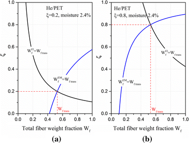

  

  Relations between $\varsigma$ and $W_{\text{f}}$ when $W_{\text{f}}^{EI} = W_{\text{f trans}}$ or $W_{\text{f}}^{EM} = W_{\text{f trans}}$ for UD distributed He/PET with $\xi$ = 0.2 (a), 0.4 (b) and moisture 2.4%

• b) Stiffness

  The influence of the agglomeration parameter $\varsigma$ on UD distributed He/PET’s $E_{L}$ can be found from Fig. 5, which are analyzed in “Longitudinal stiffness of UD distributed He/PET” section. As for the transverse stiffness $E_{T}$ with respect to fiber weight fraction $W_{\text{f}}$, the curves with different $(\varsigma ,\xi )$ are displayed in Fig. 12. It is noticed that two conditions need to be satisfied to achieve the maximum $E_{T}$. The first is uniformly distributed fiber in the composite ($\xi = \varsigma$), and the second is $W_{\text{f}} = W_{\text{f trans}}$. It is also seen that with the increasing of $\varsigma$ ($\varsigma = 0.5,\;0.52\,,\,0.6$) for composites with fixed $\xi$ ($\xi = 0.5$), the extreme high value of $E_{T}$ decreases. Besides, it also can be inferred from Fig. 12 that the aggregation of fibers is slightly beneficial to the increase in transverse stiffness of UD distributed composites at small fiber weight fraction.

  Figure 12

  

  Transverse stiffness $E_{T}$ of UD distributed He/PET composite with moisture 2.4% with respect to $W_{\text{f}}$

Additionally, influence of aggregation parameters on planar stiffness of 2D randomly distributed Fl/PP is shown in Fig. 13, as discussed in “Planar stiffness of 2D randomly distributed Fl/PP” section. In Fig. 14, their influence on 2D randomly distributed Fl/PP’s out of plane stiffness $E_{33}$ is displayed. It also implies that the aggregation in composite reduces $E_{33}$ of 2D randomly distributed composites, even at small fiber weight fraction, and the turning points in the distribution of $E_{33}$ with respect to $W_{\text{f}}$ are located at where $W_{\text{f }} = W_{\text{f trans}}$ (homogeneously fibers) or $W_{\text{f}}^{EI} = W_{\text{f trans}}$ and $W_{\text{f}}^{EM} = W_{\text{f trans}}$(non-uniform fibers) is achieved.

Figure 13

Comparison of planar stiffness of 2D randomly distributed FI/PP composite (on plane 1–2) among experimental data [41], theoretical results of this paper (with porosity) and those of Shi et al. [27] (with no porosity) (For all theoretical results, supposing that fibers are fully randomly orientated on plane 1–2, then one unique planar stiffness exists; however, in engineering, fully randomly distributed fibers are unachievable, thus two experimental stiffness are used to describe the planar stiffness, where ^{a, b}represent the planar stiffness along and transverse to the preferred fiber orientation of the nonwoven fiber mates, respectively; for results of this paper, influence of aggregation parameters $(\varsigma ,\xi )$ is considered; ^cdenotes the curves of Shi et al. [27])

Figure 14

Out of plane stiffness $E_{33}$ of 2D randomly distributed Fl/PP composite with respect to $W_{\text{f}}$

Finally, influence of aggregation parameters $(\varsigma ,\xi )$ on the Young’s modulus $E$ of 3D randomly distributed composites is studied. 3D randomly distributed Glass fiber-reinforced PP (Gl/PP) is considered in this example, and the model parameters are taken from a reference of Thomason [43], as listed in Table 1. In the calculation, the aspect ratio of the fibers is taken as 90 [18]. As depicted in Fig. 15, the maximum stiffness happens when $W_{\text{f}} = W_{\text{f trans}}$ and $\varsigma = \xi$, where no clustering exists. Besides, for fixed $\varsigma$, the increasing of $\xi$ makes the composite more uncompacted. When $\varsigma = 1$, for composites with different $\xi$($\xi =$ 0.4, 0.5, 0.6 and 1, respectively), the maximum value og stiffness increases, which are achieved when $W_{\text{f}}^{\text{EI}} = W_{\text{f trans}}$ or $W_{\text{f}} = W_{\text{f trans}}$. For fixed $\xi$ ($\xi = 0.5$) but increasing $\varsigma$($\varsigma = 0.5$, 0.52, 0.6, 0.8 and 1), due to the increasing degree of agglomeration, the maximum of composite stiffness decreases gradually. In summary, in 3D randomly distributed composites, the aggregation reduces the stiffness of the composites, even at the small fiber weight fraction ($W_{\text{f}} < W_{\text{f trans}}$ or $W_{\text{f}}^{\text{EI}} < W_{\text{f trans}}$).

Figure 15

Elastic modulus $E$ of 3D randomly distributed Gl/PP composite with respect to $W_{\text{f}}$

Conclusions

In this study, based on M–T micromechanical model, mechanical properties of three typical FRCs (3D randomly distributed FRCs, 2D randomly distributed FRCs and UD distributed ones) are investigated, taking the effect of porosity and aggregation into consideration. A novel two-parameter agglomeration model in terms of the weights of constituents is proposed to involve the relations among fiber content, porosity and agglomeration, and a two-scale approach is applied for the effective property prediction. The proposed model and method in this paper are validated by experimental data, and some valuable conclusions are made from the parameter analyses:

• 1. Porosity increases with the increase in fiber weight fraction, and there is a critical fiber weight fraction $W_{\text{f trans}}$ for a composite characterized as a perfect situation with high fiber weight fraction but low porosity. Porosity effect should not be neglected, especially for composites with fiber content higher than $W_{\text{f trans}}$.

• 2. Local aggregation of reinforcements affects the variation of stiffness with respect to the fiber weight fraction of the composite pronouncedly, in that it affects the value of total fiber weight fraction where $W_{\text{f }} = W_{\text{f trans}}$ is achieved for composites with homogeneously dispersed fibers and where $W_{\text{f}}^{\text{EI}} = W_{\text{f trans}}$ and $W_{\text{f}}^{\text{EM}} = W_{\text{f trans}}$ for composites with fiber local gathering.

• 3. With the increase in fiber content, the fiber local agglomeration in FRCs tends to increase, which weakens the stiffness of the composites significantly in general, but there is one exception that the transverse stiffness of the UD directional FRC is slightly increased with the increasing of the aggregation degree at small fiber content.

• 4. Due to the synergistic influence of the fiber content, porosity and local aggregation on FRCs’ properties, a maximum stiffness of FRCs can be achieved by making fibers uniformly dispersed in the matrix and setting the fiber weight fraction at $W_{\text{f trans}}$.

The micromechanical model and method presented in this paper have wide application potentiality in composites, in that it is applicable for composites with reinforcements ranging from nano- to macro-scale and has no limitation on their aspect ratio (0, +$\infty$). Moreover, the condition with transversely isotropic EM is involved, and more elastic constants of composites are able to be evaluated.

Appendices

Appendix 1: Eshelby tensor for a ellipsoidal inclusion in an isotropic medium

In 1957, Eshelby [34] determined the expression of Eshelby tensor ${\mathbf{S}}$ for rotational ellipsoidal inclusions in an isotropic matrix. Assuming the axis of geometrical symmetry of the ellipsoidal inclusion coincides with direction 1, and the aspect ratio is denoted by $\rho$, the original Eshelby tensor ${\mathbf{S}}$ can be represented as:

$$ {\mathbf{S}} = \left( {\begin{array}{*{20}l} {S_{{1111}} } & {S_{{1122}} } & {S_{{1122}} } & 0 & 0 & 0 \\ {S_{{2211}} } & {S_{{2222}} } & {S_{{2233}} } & 0 & 0 & 0 \\ {S_{{2211}} } & {S_{{2233}} } & {S_{{2222}} } & 0 & 0 & 0 \\ 0 & 0 & 0 & {2S_{{2323}} } & 0 & 0 \\ 0 & 0 & 0 & 0 & {2S_{{1212}} } & 0 \\ 0 & 0 & 0 & 0 & 0 & {2S_{{1212}} } \\ \end{array} } \right) $$

(31)

in which the nonzero components are expressed as:

$$ \begin{aligned} S_{1111} & = \frac{1}{{2(1 - \nu_{\text{m}} )}}\left[ {4 - 2\nu_{\text{m}} - \frac{2}{{1 - \rho^{2} }}} \right] + \frac{1}{{2(1 - \nu_{\text{m}} )}}\left[ {2\nu_{\text{m}} - 4 + \frac{3}{{1 - \rho^{2} }}} \right]q, \\ S_{2222} & = - \frac{3}{{8(1 - \nu_{\text{m}} )}}\frac{{\rho^{2} }}{{(1 - \rho^{2} )}} + \frac{1}{{4(1 - \nu_{\text{m}} )}}\left[ {1 - 2\nu_{\text{m}} + \frac{9}{{4(1 - \rho^{2} )}}} \right]q, \\ S_{2233} & = \frac{1}{{8(1 - \nu_{\text{m}} )}}\left[ {1 - \frac{1}{{(1 - \rho^{2} )}}} \right] + \frac{1}{{16(1 - \nu_{\text{m}} )}}\left[ { - 4(1 - 2\nu_{\text{m}} ) + \frac{3}{{(1 - \rho^{2} )}}} \right]q, \\ S_{2211} & = \frac{1}{{2(1 - \nu_{\text{m}} )}}\frac{{\rho^{2} }}{{(1 - \rho^{2} )}} - \frac{1}{{4(1 - \nu_{\text{m}} )}}\left[ {(1 - 2\nu_{\text{m}} ) + \frac{{3\rho^{2} }}{{(1 - \rho^{2} )}}} \right]q, \\ S_{1122} & = \frac{1}{{2(1 - \nu_{\text{m}} )}}\left[ { - (1 - 2\nu_{\text{m}} ) + \frac{1}{{(1 - \rho^{2} )}}} \right] + \frac{1}{{4(1 - \nu_{\text{m}} )}}\left[ {2(1 - 2\nu_{\text{m}} ) - \frac{3}{{(1 - \rho^{2} )}}} \right]q, \\ S_{1212} & = \frac{1}{{4(1 - \nu_{\text{m}} )}}\left[ {(1 - 2\nu_{\text{m}} ) + \frac{{1 + \rho^{2} }}{{(1 - \rho^{2} )}}} \right] - \frac{1}{{8(1 - \nu_{\text{m}} )}}\left[ {(1 - 2\nu_{\text{m}} ) + \frac{{3(1 + \rho^{2} )}}{{(1 - \rho^{2} )}}} \right]q, \\ S_{2323} & = - \frac{1}{{8(1 - \nu_{\text{m}} )}}\frac{{\rho^{2} }}{{(1 - \rho^{2} )}} + \frac{1}{{16(1 - \nu_{\text{m}} )}}\left[ {4(1 - 2\nu_{\text{m}} ) + \frac{3}{{(1 - \rho^{2} )}}} \right]q \\ \end{aligned} $$

(32)

where $\nu_{\text{m}}$ denotes the Poisson’s ratio of the isotropic matrix and

$$ q = \left\{ \begin{aligned} \frac{\rho }{{(\rho^{2} - 1)^{{{3 \mathord{\left/ {\vphantom {3 2}} \right. \kern-0pt} 2}}} }}\left[ {\rho \left( {\rho^{2} - 1} \right)^{{{1 \mathord{\left/ {\vphantom {1 2}} \right. \kern-0pt} 2}}} - {\text{arccosh}}(\rho )} \right],\quad {\text{for}}\;\rho > 1 \hfill \\ \frac{\rho }{{(1 - \rho^{2} )^{{{3 \mathord{\left/ {\vphantom {3 2}} \right. \kern-0pt} 2}}} }}\left[ {{\text{arccosh}}(\rho ) - \rho \left( {1 - \rho^{2} } \right)^{{{1 \mathord{\left/ {\vphantom {1 2}} \right. \kern-0pt} 2}}} } \right],\quad {\text{for}}\;\rho < 1 \hfill \\ \end{aligned} \right.. $$

For a spherical inclusion ($\rho = 1$), the nonzero components of Eshelby’s tensor are expressed as follows:

$$ \begin{aligned} & S_{{1111}} = S_{{3333}} = \frac{{7 - 5\nu _{{\text{m}}} }}{{15(1 - \nu _{{\text{m}}} )}}, \\ & S_{{1122}} = S_{{1133}} = S_{{2211}} = S_{{3311}} = \frac{{5\nu _{{\text{m}}} - 1}}{{15(1 - \nu _{{\text{m}}} )}}, \\ & S_{{1313}} = S_{{1212}} = \frac{{4 - 5\nu _{{\text{m}}} }}{{15(1 - \nu _{{\text{m}}} )}}. \\ \end{aligned} $$

(33)

Appendix 2: Eshelby tensor for an ellipsoidal inclusion in a transversely isotropic medium

In 1988, Withers [35] obtained the Eshelby tensor for an ellipsoidal inclusion in a transversely isotropic matrix based on the related Green’s functions provided by Pan and Chou [36]. Assuming the ellipsoidal inclusion is with aspect ratio $\rho$ and is rotationally symmetric about the direction 3 which is normal to the isotropy plane 1–2, the ${\mathbf{S}}$-tensor of that inclusion in a transversely isotropic medium $(C_{11} ,\;C_{12} ,C_{13} ,C_{33} ,C_{44} )$ can be expressed in the following matrix form:

$$ {\mathbf{S}} = \left( {\begin{array}{*{20}c} {S_{1111} } & {S_{1122} } & {S_{1133} } & 0 & 0 & 0 \\ {S_{1122} } & {S_{1111} } & {S_{1133} } & 0 & 0 & 0 \\ {S_{3311} } & {S_{3311} } & {S_{3333} } & 0 & 0 & 0 \\ 0 & 0 & 0 & {S_{1313} } & 0 & 0 \\ 0 & 0 & 0 & 0 & {S_{1313} } & 0 \\ 0 & 0 & 0 & 0 & 0 & {S_{1212} } \\ \end{array} } \right). $$

(34)

The nonzero components $S_{ijrt}$($i,j,r,t = 1,2,3$) can be written in terms of $I$ integrals as:

$$ \begin{aligned} S_{3333} & = 2\sum\limits_{i = 1}^{2} {\mu_{i}^{3} } q_{i} A_{i} '\left( {C_{13} - C_{33} q_{i} \mu_{i}^{2} } \right)I_{2} (i), \\ S_{1111} = S_{2222} & = 2\sum\limits_{i = 1}^{2} {C_{44} (1 + q_{i} )A_{i} '\mu_{i}^{3} } I_{1} (i) - C_{66} \sum\limits_{i = 1}^{2} {A_{i} '\mu_{i} I_{1} (i) + \frac{1}{2}} DC_{66} I_{1} (3), \\ S_{1122} = S_{2211} & = 2\sum\limits_{i = 1}^{2} {C_{44} (1 + q_{i} )A_{i} '\mu_{i}^{3} } I_{1} (i) - 3C_{66} \sum\limits_{i = 1}^{2} {A_{i} '\mu_{i} I_{1} (i) - \frac{1}{2}} DC_{66} I_{1} (3), \\ S_{1133} = S_{2233} & = 2\sum\limits_{i = 1}^{2} {\mu_{i} A_{i} '\left( {C_{13} - C_{33} q_{i} \mu_{i}^{2} } \right)} I_{1} (i), \\ S_{3322} = S_{3311} & = 2\sum\limits_{i = 1}^{2} {C_{44} \mu_{i}^{5} q_{i} (1 + q_{i} )A_{i} '} I_{2} (i) - 2C_{66} \sum\limits_{i = 1}^{2} {\mu_{i}^{3} q_{i} A_{i} 'I_{2} (i)} , \\ \end{aligned} $$

(35)

$$ \begin{aligned} S_{1212} & = C_{66} \sum\limits_{i = 1}^{2} {\mu_{i} A_{i} 'I_{1} (i) + \frac{1}{2}} DC_{66} I_{1} (3), \\ S_{1313} = S_{2323} & = \frac{1}{2}\sum\limits_{i = 1}^{2} {C_{44} \mu_{i}^{3} A_{i} '(1 + q_{i} )[I_{2} (i) - 2q_{i} I_{1} (i)]} + \frac{1}{4}DC_{44} I_{2} (3)\mu_{3}^{3} . \\ \end{aligned} $$

The related constants in Eq. (35) depend on the elastic constants of the transversely isotropic medium $(C_{11} ,\;C_{12} ,C_{13} ,C_{33} ,C_{44} )$ as:

$$ \begin{aligned} C_{13}^{*} & = (C_{11} C_{33} )^{{{1 \mathord{\left/ {\vphantom {1 2}} \right. \kern-0pt} 2}}} ,\;q_{i} = \frac{{{{C_{11} } \mathord{\left/ {\vphantom {{C_{11} } {\mu_{i}^{2} - C_{44} }}} \right. \kern-0pt} {\mu_{i}^{2} - C_{44} }}}}{{C_{13} + C_{44} }}, \\ \mu_{1} & = \left[ {\frac{{(C_{13}^{*} - C_{13} )(C_{13}^{*} + C_{13} + 2C_{44} )}}{{4C_{33} C_{44} }}} \right]^{{{1 \mathord{\left/ {\vphantom {1 2}} \right. \kern-0pt} 2}}} + \left[ {\frac{{(C_{13}^{*} + C_{13} )(C_{13}^{*} - C_{13} - 2C_{44} )}}{{4C_{33} C_{44} }}} \right]^{{{1 \mathord{\left/ {\vphantom {1 2}} \right. \kern-0pt} 2}}} , \\ \mu_{2} & = \left[ {\frac{{(C_{13}^{*} - C_{13} )(C_{13}^{*} + C_{13} + 2C_{44} )}}{{4C_{33} C_{44} }}} \right]^{{{1 \mathord{\left/ {\vphantom {1 2}} \right. \kern-0pt} 2}}} - \left[ {\frac{{(C_{13}^{*} + C_{13} )(C_{13}^{*} - C_{13} - 2C_{44} )}}{{4C_{33} C_{44} }}} \right]^{{{1 \mathord{\left/ {\vphantom {1 2}} \right. \kern-0pt} 2}}} , \\ \mu_{3} & = \left( {\frac{{C_{66} }}{{C_{44} }}} \right)^{{{1 \mathord{\left/ {\vphantom {1 2}} \right. \kern-0pt} 2}}} ,\;D = \frac{1}{{4\pi C_{44} \mu_{3} }},\;C_{66} = \frac{1}{2}(C_{11} - C_{12} ), \\ \mu_{1} A_{1} & = - \mu_{2} A_{2} = \frac{{C_{13} + C_{44} }}{{4\pi C_{44} C_{33} (\mu_{2}^{2} - \mu_{1}^{2} )}}, \\ A_{1} ' & = \frac{{(C_{44} - C_{33} \mu_{1}^{2} )}}{{8\pi C_{44} C_{33} (\mu_{2}^{2} - \mu_{1}^{2} )\mu_{1}^{2} }},\;A_{2} ' = - \frac{{(C_{44} - C_{33} \mu_{2}^{2} )}}{{8\pi C_{44} C_{33} (\mu_{2}^{2} - \mu_{1}^{2} )\mu_{2}^{2} }} \\ A_{i} & = - 2\mu_{i} q_{i} A_{i} '. \\ \end{aligned} $$

(36)

A degenerate case occurs when $C_{13}^{*} - C_{13} - 2C_{44} = 0$, so that $\mu_{1} = \mu_{2}.$

$I$ integrals referred to in Eq. (35) can be written with respect to the aspect ratio $\rho$ as:

$$ I_{1} (i) = 2\pi \rho^{2} \mu_{i} \int\limits_{0}^{1} {\frac{{1 - \chi^{2} }}{{\mu_{i}^{2} \rho^{2} - (\mu_{i}^{2} \rho^{2} - 1)\chi^{2} }}} {\text{d}}\chi \quad (i = 1,2,3) $$

(37)

If $\mu_{i} > {1 \mathord{\left/ {\vphantom {1 \rho }} \right. \kern-0pt} \rho }$,

$$ I_{1} (i) = \frac{2\pi \rho }{{R^{3} }}(\mu_{i} \rho R - F) $$

(38)

with $R = (\mu_{i}^{2} \rho^{2} - 1)^{{{1 \mathord{\left/ {\vphantom {1 2}} \right. \kern-0pt} 2}}}$ and $F = {\text{arccosh}}(\mu_{i} \rho )$.

If $\mu_{i} < {1 \mathord{\left/ {\vphantom {1 \rho }} \right. \kern-0pt} \rho }$,

$$ I_{1} (i) = - \frac{2\pi \rho }{{R^{3} }}(\mu_{i} \rho R - F) $$

(39)

with $R = (1 - \mu_{i}^{2} \rho^{2} )^{{{1 \mathord{\left/ {\vphantom {1 2}} \right. \kern-0pt} 2}}}$ and $F = { \arccos }(\mu_{i} \rho )$.

Additionally,

$$ I_{2} (i) = \frac{4\pi }{{\mu_{i} }}\int\limits_{0}^{1} {\frac{{\chi^{2} }}{{\mu_{i}^{2} \rho^{2} - (\mu_{i}^{2} \rho^{2} - 1)\chi^{2} }}} {\text{d}}\chi \quad (i = 1,2,3). $$

(40)

If $\mu_{i} > {1 \mathord{\left/ {\vphantom {1 \rho }} \right. \kern-0pt} \rho }$,

$$ I_{2} (i) = \frac{4\pi \rho }{{R^{3} }}\left( {F - \frac{R}{{\mu_{i} \rho }}} \right) $$

(41)

with $R = (\mu_{i}^{2} \rho^{2} - 1)^{{{1 \mathord{\left/ {\vphantom {1 2}} \right. \kern-0pt} 2}}}$ and $F = {\text{arccosh}}(\mu_{i} \rho )$.

If $\mu_{i} < {1 \mathord{\left/ {\vphantom {1 \rho }} \right. \kern-0pt} \rho }$,

$$ I_{2} (i) = - \frac{4\pi \rho }{{R^{3} }}\left( {F - \frac{R}{{\mu_{i} \rho }}} \right) $$

(42)

with $R = (1 - \mu_{i}^{2} \rho^{2} )^{{{1 \mathord{\left/ {\vphantom {1 2}} \right. \kern-0pt} 2}}}$ and $F = { \arccos }(\mu_{i} \rho )$.As a limiting case that $\mu_{i} \to 1\;(i = 1,2,3)$, the ${\mathbf{S}}$ tensor tends to the isotropic case, which was discussed in the literature of Withers [35].

References

Pyrz R, Schjødt-Thomsen J (2006) Bridging the length-scale gap—short fibre composite material as an example. J Mater Sci 41(20):6737–6750. doi:10.1007/s10853-006-0212-7
Tang JM, Lee WI, Springer GS (1987) Effects of cure pressure on resin flow, voids, and mechanical properties. J Compos Mater 21(5):421–440. doi:10.1177/002199838702100502
Leclerc JS, Ruiz E (2008) Porosity reduction using optimized flow velocity in resin transfer molding. Compos Part A Appl Sci 39(12):1859–1868. doi:10.1016/j.compositesa.2008.09.008
Li Y, Li Q, Ma H (2015) The voids formation mechanisms and their effects on the mechanical properties of flax fiber reinforced epoxy composites. Compos Part A Appl Sci 72:40–48. doi:10.1016/j.compositesa.2015.01.029
Nemat-Nasser S, Hori M (1999) Micromechanics: overall properties of heterogeneous materials, 2nd edn. Elsevier, Amsterdam
Tsukrov I, Kachanov M (2000) Effective moduli of an anisotropic material with elliptical holes of arbitrary orientational distribution. Int J Solids Struct 37(41):5919–5941. doi:10.1016/s0020-7683(99)00244-9
Herakovich CT, Baxter SC (1999) Influence of pore geometry on the effective response of porous media. J Mater Sci 34(7):1595–1609. doi:10.1023/A:1004528600213
Sevostianov I, Kushch V (2009) Effect of pore distribution on the statistics of peak stress and overall properties of porous material. Int J Solids Struct 46(25–26):4419–4429. doi:10.1016/j.ijsolstr.2009.09.002
Huang H, Talreja R (2005) Effects of void geometry on elastic properties of unidirectional fiber reinforced composites. Compos Sci Technol 65(13):1964–1981. doi:10.1016/j.compscitech.2005.02.019
Yang BJ, Ha SK, Pyo SH, Lee HK (2014) Mechanical characteristics and strengthening effectiveness of random-chopped FRC composites containing air voids. Compos Part B Eng 62:159–166. doi:10.1016/j.compositesb.2014.02.015
Liebig WV, Viets C, Schulte K, Fiedler B (2015) Influence of voids on the compressive failure behaviour of fibre-reinforced composites. Compos Sci Technol 117:225–233. doi:10.1016/j.compscitech.2015.06.020
Dong C (2016) Effects of process-induced voids on the properties of fibre reinforced composites. J Mater Sci Technol 32(7):597–604. doi:10.1016/j.jmst.2016.04.011
Zou N, Li Q (2016) Compressive mechanical property of porous magnesium composites reinforced by carbon nanotubes. J Mater Sci 51(11):5232–5239. doi:10.1007/s10853-016-9824-8
Maragoni L, Carraro PA, Peron M, Quaresimin M (2017) Fatigue behaviour of glass/epoxy laminates in the presence of voids. Int J Fatigue 95:18–28. doi:10.1016/j.ijfatigue.2016.10.004
Pines ML, Bruck HA (2006) Pressureless sintering of particle-reinforced metal–ceramic composites for functionally graded materials: part I. Porosity reduction models. Acta Mater 54(6):1457–1465. doi:10.1016/j.actamat.2005.10.060
Madsen B, Lilholt H (2003) Physical and mechanical properties of unidirectional plant fibre composites—an evaluation of the influence of porosity. Compos Sci Technol 63(9):1265–1272. doi:10.1016/s0266-3538(03)00097-6
Madsen B, Thygesen A, Lilholt H (2007) Plant fibre composites–porosity and volumetric interaction. Compos Sci Technol 67(7–8):1584–1600. doi:10.1016/j.compscitech.2006.07.009
Madsen B, Thygesen A, Lilholt H (2009) Plant fibre composites–porosity and stiffness. Compos Sci Technol 69(7–8):1057–1069. doi:10.1016/j.compscitech.2009.01.016
Mackenzie JK (1950) The elastic constants of a solid containing spherical holes. Proc Phys Soc 63(1):2–11. doi:10.1088/0370-1301/63/1/302
Liu Y, Kumar S (2014) Polymer/carbon nanotube nano composite fibers—a review. ACS Appl Mater Inter 6(9):6069–6087. doi:10.1021/am405136s
Kamarian S, Salim M, Dimitri R, Tornabene F (2016) Free vibration analysis of conical shells reinforced with agglomerated carbon nanotubes. Int J Mech Sci 108–109:157–165. doi:10.1016/j.ijmecsci.2016.02.006
Zhu J, Kim JD, Peng H, Margrave JL, Khabashesku VN, Barrera EV (2003) Improving the dispersion and integration of single-walled carbon nanotubes in epoxy composites through functionalization. Nano Lett 3(8):1107–1113. doi:10.1021/nl034248
Zhao S, Song ZX, Cui J, Li CQ, Yan YH (2012) Improving dispersion and integration of single-walled carbon nanotubes in epoxy composites by using a reactive noncovalent dispersant. J Polym Sci Polym Chem 50(21):4548–4556. doi:10.1002/pola.26267
Mikhalchan A, Gspann T, Windle A (2016) Aligned carbon nanotube–epoxy composites: the effect of nanotube organization on strength, stiffness, and toughness. J Mater Sci 51(22):10005–10025. doi:10.1007/s10853-016-0228-6
Dzenis YA (1986) Effect of aggregation of a dispersed rigid filler on the elastic characteristics of a matrix composite. Mech Compos Mater 22(1):12–19. doi:10.1007/bf00606002
Dorigato A, Dzenis Y, Pegoretti A (2013) Filler aggregation as a reinforcement mechanism in matrix nanocomposites. Mech Mater 61:79–90. doi:10.1016/j.mechmat.2013.02.004
Shi DL, Feng XQ, Huang YY, Hwang KC, Gao HJ (2004) The effect of nanotube waviness and agglomeration on the elastic property of carbon nanotube-reinforced composites. J Eng Mater T 126(3):250–257. doi:10.1115/1.1751182
Gkikas G, Barkoula NM, Paipetis AS (2012) Effect of dispersion conditions on the thermo-mechanical and toughness properties of multi walled carbon nanotubes-reinforced epoxy. Compos Part B Eng 43(6):2697–2705. doi:10.1016/j.compositesb.2012.01.070
Pourasghar A, Yas MH, Kamarian S (2013) Local aggregation effect of CNT on the vibrational behavior of four-parameter continuous grading nanotube-reinforced cylindrical panels. Polym Compos 34(5):707–721. doi:10.1002/pc.22474
Kamarian S, Salim M, Dimitri R, Tornabene F (2016) Free vibration analysis of conical shells reinforced with agglomerated carbon nanotubes. Int J Mech Sci 108:157–165. doi:10.1016/j.ijmecsci.2016.02.006
Dai HL, Mei C, Rao YN (2016) A novel method for prediction of tensile strength of spherical particle-filled matrix composites with strong adhesion. Polym Eng Sci. doi:10.1002/pen.24393
Slipenyuk A, Kuprin V, Milman Y, Goncharuk V, Eckert J (2006) Properties of P/M processed particle reinforced metal matrix composites specified by reinforcement concentration and matrix-to-reinforcement particle size ratio. Acta Mater 54:157–166. doi:10.1016/j.actamat.2005.08.036
Mori T, Tanaka K (1973) Average stress in matrix and average elastic energy of materials with misfitting inclusions. Acta Metall 21(5):571–574. doi:10.1016/0001-6160(73)90064-3
Eshelby JD (1957) The determination of the elastic field of an ellipsoidal inclusion, and related problems. Proc R Soc Lond A R Soc 241:376–396. doi:10.1007/1-4020-4499-2_18
Withers PJ (1989) The determination of the elastic field of an ellipsoidal inclusion in a transversely isotropic medium, and its relevance to composite materials. Philos Mag A 59(4):759–781. doi:10.1080/01418618908209819
Pan YC, Chou TW (1976) Point force solution for an infinite transversely isotropic solid. Int J Appl Mech 43(4):608–612. doi:10.1115/1.3423941
Walpole LJ (1969) On the overall elastic moduli of composite materials. J Mech Phys Solids 17:235–251. doi:10.1016/0022-5096(69)90014-3
Walpole LJ (1981) Elastic behavior of composite materials: theoretical foundations. Adv Appl Mech 21:169–242. doi:10.1016/s0065-2156(08)70332-6
Rao YN, Dai HL (2017) Micromechanics-based thermo-viscoelastic properties prediction of fiber reinforced polymers with graded interphases and slightly weakened interfaces. Compos Struct 168:440–455. doi:10.1016/j.compstruct.2017.02.059
Madsen B (2004) Properties of plant fibre yarn matrix composites—an experimental study. Ph.D. thesis, Technical University of Denmark, Copenhagen, Denmark
Toftegaard H (2002) Tensile testing of flax/PP laminates. Risø Report: Risø-I-1799(EN). Risø National Laboratory, Materials Research Department, Denmark
Hull D, Clyne TW (1996) An introduction to composite materials, 2nd edn. Cambridge University Press, Cambridge
Thomason JL (2005) The influence of fibre length and concentration on the properties of glass fibre reinforced polypropylene: 6. The properties of injection moulded long fibre PP at high fibre content. Compos Part A Appl Sci 36(7):995–1003. doi:10.1016/j.compositesa.2004.11.004
Acknowledgements
The authors gratefully acknowledge the support of National Natural Science Foundation of China (11372105), Hunan Provincial Natural Science Foundation of China (2017JJ2044), State Key Laboratory of Advanced Design and Manufacturing for Vehicle Body (71475004) and Hunan Provincial Innovation Foundation for Postgraduate (CX2014B156).
Author information
Authors and Affiliations
Corresponding author