Characterization of Graph-Based Hierarchical Watersheds: Theory and Algorithms

Abstract

Watershed is a well-established clustering and segmentation method. In this article, we aim to achieve a better theoretical understanding of the hierarchical version of the watershed operator. More precisely, we propose a characterization of hierarchical watersheds in the framework of edge-weighted graphs. The proposed characterization leads to an efficient algorithm to recognize hierarchical watersheds.

1 Introduction

Hierarchical clustering has a long history in data processing [11]. In image processing, it is called hierarchical image segmentation [32]. Given an initial partition, a hierarchy is created by successively merging neighbouring regions together. In practice, a common way to create the initial partition is often to use the watershed operator [4, 8, 23, 24], whether we are dealing with data [5] or images. When merging the regions (called catchment basins in this context) of an initial watershed segmentation in a sequence provided by a given total ordering (such as for instance [34]), we obtain a hierarchical watershed [3, 7, 22, 28]. The watershed operator is still widely used in today’s deep learning era as a pre-processing [13] or post-processing step [1], achieving state-of-the-art results.

In the framework of edge-weighted graphs, hierarchical watersheds benefit from many interesting theoretical and practical properties [6, 9]. In particular, they globally optimize a well-defined cost function, both for the original graph and for every partition of the hierarchy, and they can be computed by efficient algorithms such as the ones proposed in [6, 26], whose time complexity is the same as minimum spanning tree algorithms. In order to leverage from those properties in a practical context, we study in this paper the problem of recognizing hierarchical watersheds. More precisely, we aim to solve the following problem:

(P):

given a weighted graph and a hierarchy of partitions ${\mathcal {H}}$, determine if ${\mathcal {H}}$ is a hierarchical watershed of this graph.

Solving this problem has a strong potential impact on the practice. It can help us, for example, in designing an algorithm to transform any hierarchy of partitions into a hierarchical watershed [17].

The problem of recognizing hierarchical watersheds is related to the one studied in [2, 12]. In [2, 12], the authors search for a minimum set of markers which lead to a given watershed segmentation. In our case, given a hierarchy, we investigate if, for every partition $\mathbf{P }$ of this hierarchy, there is a subset ${\mathcal {M}}$ of the set of the minima of the graph such that $\mathbf{P }$ is the watershed segmentation for ${\mathcal {M}}$ (Sect. 2.3). In the affirmative case, the given hierarchy is a hierarchical watershed or at least a hierarchy composed of partitions of a hierarchical watershed, which we call a flattened hierarchical watershed (Sect. 5).

This article is an extension of the conference paper [16]. Our main contributions are the following: (1) a characterization of hierarchical watersheds in the framework of weighted graphs (Theorem 5); (2) an efficient algorithm to recognize hierarchical watersheds (Algorithm 1); (3) the study of the notion of flattened hierarchical watersheds and an algorithm to recognize such hierarchies (Algorithm 2); and (4) experimental results with the proposed algorithms applied to the combinations of hierarchical watersheds assessed in [14]. To ease the reading of the paper, proofs of the various properties and theorems are postponed to “Appendix”.

In Sect. 2, we present the basic notions for handling hierarchies with graphs. In Sect. 3, we formally state the problem of recognizing hierarchical watersheds and we present a characterization of hierarchical watersheds on arbitrary graphs. In Sect. 4, we present an efficient algorithm to recognize hierarchical watersheds. In Sect. 5, we introduce the notion of flattened hierarchical watersheds, which are hierarchies composed of a subset of the partitions of a hierarchical watershed. Then, we propose an algorithm that recognizes this type of hierarchy. In Sect. 6, we present some experimental results using the proposed algorithms. Finally, we conclude the paper, in particular, by providing a glimpse on a possible extension of this work in the design of a watersheding operator [17].

2 Background Notions

In this section, we first introduce hierarchies of partitions. Then, we review the definition of graphs, connected hierarchies and saliency maps. Subsequently, we define hierarchical watersheds.

2.1 Hierarchies of Partitions

Let V be a set. A partition (of V) is a set $\mathbf{P }$ of non empty disjoint subsets of V whose union is V. Any element of a partition $\mathbf{P }$ is called a region of $\mathbf{P }$. Let $\mathbf{P }_1$ and $\mathbf{P }_2$ be two partitions. We say that $\mathbf{P }_1$ is a refinement of $\mathbf{P }_2$ if every element of $\mathbf{P }_1$ is included in an element of $\mathbf{P }_2$. A hierarchy (of partitions) is a sequence ${\mathcal {H}} =(\mathbf{P }_0, \ldots , \mathbf{P }_\ell )$ of partitions such that $\mathbf{P }_{i-1}$ is a refinement of $\mathbf{P }_{i}$, for any i in $\{1, \ldots , \ell \}$ and such that $\mathbf{P }_n = \{V\}$. Let ${\mathcal {H}}=(\mathbf{P }_0, \ldots , \mathbf{P }_{\ell })$ be a hierarchy of partitions. Any region of a partition $\mathbf{P }$ of ${\mathcal {H}}$ is called a region of ${\mathcal {H}}$.

A hierarchy of partitions can be represented as a tree whose nodes correspond to regions, as shown in Fig. 1a. Given a hierarchy ${\mathcal {H}}$ and two regions X and Y of ${\mathcal {H}}$, we say that Xis a parent ofY(or thatYis a child ofX) if $Y \subset X$ and X is minimal for this property, i.e. if there is a region Z such that $Y \subseteq Z \subset X$, then we have $Y=Z$. It can be seen that any region $X\ne V$ of ${\mathcal {H}}$ has exactly one parent. For any region X such that $X \ne V$, we write $parent(X)=Y$ where Y is the unique parent of X. For any region R of ${\mathcal {H}}$, if R is not the parent of any region of ${\mathcal {H}}$, we say that Ris a leaf region (of${\mathcal {H}}$). Otherwise, we say that Ris a non-leaf region (of ${\mathcal {H}}$).

In Fig. 1a, the regions of a hierarchy ${\mathcal {H}}$ are linked to their parents (and to their children) by straight lines.

Fig. 1

a A representation of a hierarchy of partitions ${\mathcal {H}}=(\mathbf{P }_0, \mathbf{P }_1, \mathbf{P }_2, \mathbf{P }_3)$ on the set $\{a,b,c,d,e,f,g,h\}$. b A weighted graph (G, w)

2.2 Graphs, Connected Hierarchies and Saliency Maps

A graph is a pair $G=(V, E)$, where V is a finite set and E is a set of pairs of distinct elements of V, i.e. $E \subseteq \{\{x,y\} \subseteq V \mid x \ne y\}$. Each element of V is called a vertex (of G), and each element of E is called an edge (of G). To simplify the notation, the set of vertices and edges of a graph G will be also denoted by V(G) and E(G), respectively.

Let $G= (V,E)$ be a graph, and let X be a subset of V. A sequence $\pi =( x_0, \ldots , x_n)$ of elements of X is a path (in X) from $x_0$to $x_n$ if $\{x_{i-1},x_i\}$ is an edge of G for any i in $\{1, \ldots , n\}$. Given a path $\pi =( x_0, \ldots , x_n)$, for any i in $\{1, \ldots , n\}$, we say that $u=\{x_{i-1},x_i\}$is an edge in$\pi$ and that uis in$\pi$. The subset X of V is said to be connected if, for any x and y in X, there exists a path from x to y. The subset X is a connected component of G if X is connected and maximal. In the following, we denote by CC(G) the set of all connected components of G. This set CC(G) of all connected components of G is a partition of the set V.

Let $G = (V,E)$ be a graph. A partition of Vis connected for G if each of its regions is connected, and a hierarchy on Vis connected (for G) if every one of its partitions is connected. For example, the hierarchy of Fig. 1a is connected for the graph of Fig. 1b.

Let G be a graph. If w is a map from the edge set of G to the set $\mathbb {R}$ of real numbers, then the pair (G, w) is called an (edge) weighted graph. If (G, w) is a weighted graph, for any edge u of G, the value w(u) is called the weight of u(for w).

Important notation in the remaining part of this article, the symbol (G, w) denotes a weighted graph whose vertex set is connected. To shorten the notation, the vertex set of G is denoted by V and its edge set is denoted by E. Without loss of generality, we also assume that the range of w is included in the set $\mathbb {E}$ of all integers from 0 to $|E|-1$. (Otherwise, one could always consider an increasing one-to-one correspondence from the set $\{w(u) \mid u \in E\}$ into the subset $\{0,...,| \{w(u) \mid u \in E\}|-1\}$ of $\mathbb {E}$.)

Let $\lambda$ be any element in $\mathbb {R}$. The $\lambda$-level set of (G, w) is the graph $(V,E_{\lambda }(G))$ such that $E_{\lambda }(G)=\{u \in E(G)\ | \ w(u)\le \lambda \}$. The sequence

$$\begin{aligned} \mathcal {QFZ}(w) = (CC(G_{\lambda ,w}) \mid \lambda \in \mathbb {E}) \end{aligned}$$

(1)

where $G_{\lambda ,w}$ is the $\lambda$-level set of (G, w), is a hierarchy called the quasi-flat zones (QFZ) hierarchy (of w) [6, 20, 25, 33].

As established in [9], a connected hierarchy can be equivalently treated by means of a weighted graph through the notion of a (contour) saliency map. Given a hierarchy ${\mathcal {H}} = (\mathbf{P }_0, \ldots , \mathbf{P }_\ell )$ which is connected for G, the saliency map of ${\mathcal {H}}$ is the map from E into $\{0, \ldots , \ell \}$, denoted by $\varPhi ({\mathcal {H}})$, such that, for any edge $u=\{x, y\}$ in E, the value $\varPhi ({\mathcal {H}})(u)$ is the lowest value i in $\{0, \ldots , \ell \}$ such that x and y belong to a same region of $\mathbf{P }_{i}$. It follows that any connected hierarchy has a unique saliency map. Moreover, any hierarchy ${\mathcal {H}}$ connected for G is precisely the quasi-flat zones hierarchy of its own saliency map: ${\mathcal {H}} = \mathcal {QFZ}(\varPhi ({\mathcal {H}}))$.

For instance, the map depicted in Fig. 1b is the saliency map of the hierarchy of Fig. 1a.

Saliency maps are closely related to the notion of ultrametric distances [1, 27]. Let ${\mathcal {H}}$ be a hierarchy on V. Let d be a map from $V \times V$ into $\mathbb {R}$ such that, for any pair (x, y) of vertices in $V \times V$, the value d(x, y) is the greatest edge weight $\lambda$ in a path $\pi$ from x to y (resp. y to x) in $(G, \varPhi ({\mathcal {H}}))$ such that, for any other path $\pi '$ from x to y (resp. y to x), the greatest edge weight in $\pi '$ is greater than or equal to $\lambda$. We can affirm that (V, d) is an ultrametric space. Moreover, for any two vertices x and y in V, by the definition of saliency maps, we may say that d(x, y) is the lowest value $\lambda$ such that x and y belong to a same region of the partition $\mathbf{P }_\lambda$ of ${\mathcal {H}}$. Furthermore, if G is a complete graph, we can conclude that $(V,\varPhi ({\mathcal {H}}))$ is an ultrametric space.

2.3 Hierarchical Minimum Spanning Forests and Watersheds

The watershed segmentation, see, for example, [4, 8, 28], derives from the topographic notion of watershed lines and catchment basins. In [8], the authors formalize watersheds in the framework of (edge) weighted graphs and show the optimality of watersheds in the sense of minimum spanning forests. In this section, we present hierarchical watersheds following the definition of hierarchies of minimum spanning forests presented in [6, 7].

We say that the graph $G=(V,E)$is a forest if, for any edge u in E, the number of connected components of the graph $(V, E{\setminus } \{u\})$ is greater than the number of connected components of G. Given another graph $G_s$, we say that $G_s$is a subgraph of G, denoted by $G_s \sqsubseteq G$, if $V(G_s)$ is a subset of V and if $E(G_s)$ is a subset of E. Let $G_1$ be a subgraph of G and let $G_2$ be a subgraph of $G_1$. The graph $G_1$ is a minimum spanning forest (MSF) of Grooted in $G_2$ if:

• 1. the graphs G and $G_1$ have the same set of vertices, i.e.  $V(G_1) = V$; and

• 2. each connected component of $G_1$ includes exactly one connected component of $G_2$; and

• 3. the sum of the weight of the edges of $G_1$ is minimal among all subgraphs of G for which the above conditions 1 and 2 hold true.

Given a path $(x_0, \ldots , x_n)$ in G, we say that $\pi$is a cycle if $x_0$ and $x_n$ are equal and if the edges in $\pi$ are pairwise distinct. A MSF of (G, w) rooted in a single vertex of G and which does not contain any cycles is a tree (connected forest) called a minimum spanning tree (MST) of (G, w).

Let k be a value in $\mathbb {R}$. A connected subgraph ${G_s}$ of G is a (regional) minimum (of w) at level k if:

• 1. the set of edges ${E(G_s)}$ of ${G_s}$ is not empty; and

• 2. for any edge u in ${E(G_s)}$, the weight of u is equal to k; and

• 3. for any edge $\{x,y\}$ in $E{\setminus } {E(G_s)}$ such that $| \{x,y\} \cap {V(G_s)} | \ge 1$, the weight of $\{x,y\}$ is strictly greater than k.

Important notation in the remaining part of this article, we denote by n the number of minima of w. Every sequence of minima of w considered in this article is a sequence of n pairwise distinct minima of w and, therefore, for the sake of simplicity, we use the term sequence of minima ofw instead of sequence ofnpairwise distinct minima ofw.

Let $\{G_1, \ldots , G_{\ell }\}$ be a set of graphs. We denote by $\sqcup \{G_1, \ldots , G_{\ell }\}$ the graph $( \cup \{V(G_j) \mid j \in \{1, \ldots , \ell \}\}, \cup \{E(G_j) \mid j \in \{1, \ldots , \ell \}\})$. In the following, we define hierarchical watersheds based on minimum spanning forests, as done in [6, 7].

Definition 1

(Hierarchical watershed [6, 7]) Let ${\mathcal {S}} = (M_1, \ldots , M_n)$ be a sequence of minima of w. Let $(G_0, \ldots , G_{n-1})$ be a sequence of subgraphs of G such that:

• 1. for any i in $\{0, \ldots , n-1\}$, the graph $G_i$ is a MSF of G rooted in $\sqcup \{M_j \mid j \in \{i+1, \ldots , n\}\}$; and

• 2. for any i in $\{1, \ldots , n-1\}$, $G_{i-1}$ is a subgraph of $G_i$.

The sequence ${\mathcal {T}} = (CC(G_0), \ldots , CC(G_{n-1}))$ is called a hierarchical watershed of (G, w) for ${\mathcal {S}}$. Given a hierarchy ${\mathcal {H}}$, we say that ${\mathcal {H}}$is a hierarchical watershed of (G, w) if there exists a sequence ${\mathcal {S}}$ of minima of w such that ${\mathcal {H}}$ is a hierarchical watershed of (G, w) for ${\mathcal {S}}$.

For instance, let (G, w) and ${\mathcal {H}}$ be, respectively, the weighted graph and the hierarchy shown in Fig. 2a, b, respectively. We can see that ${\mathcal {H}}$ is the hierarchical watershed of (G, w) for the sequence (C, A, B, D) of minima of w.

Fig. 2

a A weighted graph (G, w) with four minima delimited by the dashed lines. b The hierarchical watershed of (G, w) for the sequence (C, A, B, D) of minima of w. c The unique binary partition hierarchy ${\mathcal {B}}$ of (G, w)

3 Characterization of Hierarchical Watersheds

In this section, we solve the following recognition problem:

(P):

given a weighted graph (G, w) and a hierarchy of partitions ${\mathcal {H}}$, determine if ${\mathcal {H}}$ is a hierarchical watershed of (G, w).

A naive approach to solve Problem (P) is to test if there is a sequence ${\mathcal {S}}$ of minima of w such that ${\mathcal {H}}$ is the hierarchical watershed of (G, w) for ${\mathcal {S}}$. However, there exist n! sequences of minima of w, which leads to an algorithm of factorial time complexity.

To solve Problem (P) more efficiently, we propose in Sect. 3.2 a characterization of hierarchical watersheds (Lemma 4) based on the binary partition hierarchy by altitude ordering (Sect. 3.1) which, as stated in [6], is known to be closely related to hierarchical watersheds. Then, we present a sketch of the proof of Lemma 4 by linking one-side increasing maps to the notion of extinction values as defined in [6]. Based on our proposed characterization of hierarchical watersheds, we design an efficient algorithm (Algorithm 1) to solve Problem (P).

3.1 Binary Partition Hierarchies by Altitude Ordering

Binary partition trees [30] are widely used for hierarchical image representation. In this section, we describe the case where regions linked by the lowest edge weights are the first regions to be merged in the hierarchy [6]. As stated in [9], this particular case is deeply connected to single-linkage clustering.

Let $\prec$ be a total ordering (on E), i.e. $\prec$ is a binary relation that is transitive and trichotomous: for any u and v in E only one of the relations $u \prec v$, $v \prec u$ and $v = u$ holds true. We say that $\prec$is an altitude ordering (on E) for w if, for any u and v in E such that $w(u) < w(v)$, we have $u \prec v$. Hence, given an altitude ordering $\prec$ for w and given any two edges u and v such that $w(u) = w(v)$, we can have either $u \prec v$ or $v \prec u$. Let $\prec$ be an altitude ordering for w. Let k be any element in $\{1,\ldots ,|E|\}$. We denote by $u_k^{\prec }$ the k-th element of E with respect to $\prec$. We set $\mathbf{B }_0 = \{\{x\} \mid x \in V\}$. The k-partition of V(by the ordering $\prec$) is defined by $\mathbf{B }_k = \{ \mathbf{B }_{k-1}^y \cup \mathbf{B }_{k-1}^x \} \cup (\mathbf{B }_{k-1} {\setminus } \{\mathbf{B }_{k-1}^x, \mathbf{B }_{k-1}^y\})$ where $u_k^{\prec } = \{x,y\}$ and $\mathbf{B }_{k-1}^x$ and $\mathbf{B }_{k-1}^y$ are the regions of $\mathbf{B }_{k-1}$ that contain x and y, respectively. The sequence $(\mathbf{B }_i \mid i=0\ or\ \mathbf{B }_i \ne \mathbf{B }_{i-1})$, denoted by ${\mathcal {B}}_\prec$, is a hierarchy on V called the binary partition hierarchy (by altitude ordering) of (G, w) by $\prec$. We can observe that successive k-partitions can be equal. In such case, only one of the repeated partitions is in ${\mathcal {B}}_\prec$.

Let ${\mathcal {B}}$ be a hierarchy on V. We say that ${\mathcal {B}}$is a binary partition hierarchy (by altitude ordering) of (G, w) if there is an altitude ordering $\prec$ for w such that ${\mathcal {B}}$ is the binary partition hierarchy of (G, w) by $\prec$.

Let $\prec$ be an altitude ordering for w. We can associate any non-leaf region X of the binary partition hierarchy ${\mathcal {B}}_{\prec }$ of (G, w) by $\prec$ to the lowest rank r such that $\mathbf{B }_r$ contains X. This rank is called the rank of X. Let X be a non-leaf region of ${\mathcal {B}}_{\prec }$ and let r be the rank of X. The building edge of X is the r-th edge for $\prec$. Given an edge u in E, if u is the building edge of a region of ${\mathcal {B}}_{\prec }$, we say that uis a building edge for $\prec$. Given a building edge u for $\prec$, we denote the region of ${\mathcal {B}}_{\prec }$ whose building edge is u by $R_u$. The set of all building edges for $\prec$ is denoted by $E_{\prec }$.

Let (G, w) be the weighted graph illustrated in Fig. 2a and let ${\mathcal {B}}$ be the binary partition hierarchy of (G, w) illustrated in Fig. 2c. We can see that ${\mathcal {B}}$ is the binary partition hierarchy of (G, w) by the altitude ordering $\prec$ such that $\{a,b\} \prec \{c,d\} \prec \{e,f\} \prec \{g,h\} \prec \{a,c\} \prec \{e,g\} \prec \{c,e\}$. The building edge of each non-leaf region R of ${\mathcal {B}}$ is shown above the node that represents R.

Let ${\mathcal {B}}$ be a binary partition hierarchy of (G, w) and let X and Y be two distinct regions of ${\mathcal {B}}$. If the parent of X is equal to the parent of Y, we say that X is a sibling of Y, that Y is a sibling of X and that X and Y are siblings. It can be seen that any region $R \ne V$ of ${\mathcal {B}}$ has exactly one sibling and we denote this unique sibling of R by sibling(R).

Important remark by abuse of terminology, when no confusion is possible, if M is a minimum of w, we call the set V(M) of vertices of M as a minimum of w.

As established in [26], given an altitude ordering $\prec$ for w, the minima of w can be extracted from the binary partition hierarchy ${\mathcal {B}}_\prec$ as well as the watershed-cut edges for $\prec$, whose definition is given bellow.

Definition 2

(Watershed-cut edge) Let $\prec$ be an altitude ordering for w and let u be a building edge for $\prec$. We say that uis a watershed-cut edge (of (G, w)) for $\prec$ if each child of the region $R_u$ of ${\mathcal {B}}_\prec$ includes at least one minimum of w.

3.2 Characterization of Hierarchical Watersheds

In [16], the authors propose a characterization of hierarchical watersheds in the following case: the given graph is a tree with pairwise distinct edge weights. In this section, we generalize the characterization of hierarchical watersheds introduced in [16] to arbitrary graphs. To ease the reading of this section, the proofs of the properties and theorems stated here are delayed to “Appendix”.

Let $\prec$ be an altitude ordering for w and let f be a map from E into $\mathbb {R}$. The supremum descendant value of Rfor fand $\prec$ is the supremum edge weight among the building edges of the regions included in R: $\vee \{f(v)\ |\ v \in E_\prec , R_v \subseteq R\}$, where $\vee$ maps any set of values into the supremum value in this set, and the supremum of an empty set is zero.

The next definition introduces the notion of one-side increasing map. As established later in Lemma 4, the notion of one-side increasing map is linked to the saliency maps of hierarchical watersheds.

Definition 3

(One-side increasing map) Let $\prec$ be an altitude ordering for w and let f be a map from E into $\mathbb {R}$. We say that f is one-side increasing for $\prec$ if:

• 1. $\{f(u) \mid u \in E_\prec \}=\{0, \ldots , n-1\}$;

• 2. for any edge u in $E_\prec$, the weight f(u) is greater than zero if and only if u is a watershed-cut edge for $\prec$; and

• 3. for any edge u in $E_\prec$, there exists a child R of $R_u$ such that f(u) is greater than or equal to the supremum descendant value of R for f and $\prec$.

The next lemma, whose proof is given in “Appendix F”, states that hierarchical watersheds can be characterized as the hierarchies whose saliency maps are one-side increasing maps.

Lemma 4

Let ${\mathcal {H}}$ be a hierarchy on V. The hierarchy ${\mathcal {H}}$ is a hierarchical watershed of (G, w) if and only if there is an altitude ordering $\prec$ for w such that the saliency map $\varPhi ({\mathcal {H}})$ is one-side increasing for $\prec$.

Let ${\mathcal {H}}$ be the hierarchy of Fig. 3a, let $\varPhi ({\mathcal {H}})$ be the saliency map of ${\mathcal {H}}$ shown in Fig. 3b, and let ${\mathcal {B}}$ be the binary partition hierarchy of (G, w) (Fig. 2) shown in Fig. 3b. As the edges of G have pairwise distinct weights for w, we can conclude that ${\mathcal {B}}$ is the binary partition hierarchy of (G, w) by the unique altitude ordering $\prec$ for w. We can verify that $\varPhi ({\mathcal {H}})$ is one-side increasing for $\prec$. By Lemma 4, we may affirm that $\varPhi ({\mathcal {H}})$ is the saliency map of a hierarchical watershed of (G, w) and that, consequently, the hierarchy ${\mathcal {H}}$ is a hierarchical watershed of (G, w).

Let us now consider the hierarchy ${\mathcal {H}}'$ and the saliency map $\varPhi ({\mathcal {H}}')$ of Fig. 3d, e, respectively. We can see that $\varPhi ({\mathcal {H}}')$ is not one-side increasing for $\prec$. Indeed, the weight $\varPhi ({\mathcal {H}}')(\{c,e\})$ of the building edge of the region $Y_7$ of ${\mathcal {B}}$ is 1, which is lower than both $\vee \{\varPhi ({\mathcal {H}}')(v) \mid R_v \subseteq Y_5\}=2$ and $\vee \{\varPhi ({\mathcal {H}}')(v) \mid R_v \subseteq Y_6\}=3$. Hence, the condition 3 of Definition 3 is not satisfied by $\varPhi ({\mathcal {H}}')$. Thus, by Lemma 4, as $\prec$ is the unique altitude ordering for w, we may deduce that $\varPhi ({\mathcal {H}}')$ is not the saliency map of a hierarchical watershed of (G, w) and that ${\mathcal {H}}'$ is not a hierarchical watershed of (G, w).

Fig. 3

a, d The hierarchies ${\mathcal {H}}$ and ${\mathcal {H}}'$, respectively. b, e The weighted graphs $(G,\varPhi ({\mathcal {H}}))$ and $(G,\varPhi ({\mathcal {H}}'))$, respectively. c, f The maps $\varPhi ({\mathcal {H}})$ and $\varPhi ({\mathcal {H}}')$ represented on the hierarchy ${\mathcal {B}}$ of Fig. 2c, where, for each edge u, the values $\varPhi ({\mathcal {H}})(u)$ and $\varPhi ({\mathcal {H}}')(u)$ are shown above the region $R_u$ of ${\mathcal {B}}$

In the case where (G, w) has pairwise distinct edge weights, there exists a unique altitude ordering for w. Hence, we can use Lemma 4 to verify that a given map f is the saliency map of a hierarchical watershed of (G, w) by simply checking if f is one-side increasing for the unique altitude ordering for w. Otherwise, let us consider that (G, w) has arbitrary edge weights. Thus, in order to test if a map f is the saliency map of a hierarchical watershed of (G, w), we need to test if there is an altitude ordering $\prec$ for w such that f is one-side increasing for $\prec$. In the worst case, there exist |E|! possible altitude orderings for w. Hence, the naive approach to verify that f is one-side increasing for an altitude ordering for w has a factorial time complexity, which is the same time complexity as the algorithm to verify that f is the saliency map of a hierarchical watershed for a sequence of minima of w. Actually, as we establish later in Theorem 5, it is sufficient to test if f is one-side increasing for a single altitude ordering for w, which is the key idea behind our efficient algorithm (Algorithm 1) to recognize hierarchical watersheds.

Let f and g be two maps from E into $\mathbb {R}$. A lexicographic ordering for (f, g) is a total ordering $\prec$ on E such that, for any two edges u and v in E, we have $u \prec v$ if $f(u) < f(v)$ or if $f(u) = f(v)$ and $g(u) \le g(v)$. We can note that any lexicographic ordering for (f, g) is an altitude ordering for f.

Theorem 5

Let ${\mathcal {H}}$ be a hierarchy on V and let $\prec$ be a lexicographic ordering for $(w,{\varPhi ({\mathcal {H}})})$. The hierarchy ${\mathcal {H}}$ is a hierarchical watershed of (G, w) if and only if $\varPhi ({\mathcal {H}})$ is one-side increasing for $\prec$.

The following is a sketch of the proof of Theorem 5, whose formal proof is given in “Appendix B”. Given any hierarchy ${\mathcal {H}}$ and any altitude ordering $\prec$ for w, we can obtain a lexicographic ordering for $(w, \varPhi ({\mathcal {H}}))$ by iteratively reordering the pairs of edges (u, v) such that $u \prec v$ and such that $\varPhi ({\mathcal {H}})(u) \ge \varPhi ({\mathcal {H}})(v)$, similar to the sorting steps of the bubble sort algorithm. Let $\prec '$ be an altitude ordering resulting from the reordering of two edges u and v such that $u \prec v$ and such that $\varPhi ({\mathcal {H}})(u) \ge \varPhi ({\mathcal {H}})(v)$. To prove Theorem 5, we prove that, if $\varPhi ({\mathcal {H}})$ is one-side increasing for $\prec$, then $\varPhi ({\mathcal {H}})$ is also one-side increasing for $\prec '$. For each reordering, we prove that the three statements of Definition 3 for $\varPhi ({\mathcal {H}})$ to be one-side increasing still hold true in the following five cases: (a) neither u nor v is a building edge for $\prec$ (Lemma 30); (b) both u and v are building edges for $\prec$ and $R_u \cap R_v = \emptyset$ (Lemma 31); (c) both u and v are building edges for $\prec$ and $R_u \subset R_v$ (Lemma 32); (d) only u is a building edge for $\prec$ (Lemma 33); and (e) only v is a building edge for $\prec$ (Lemma 34).

In the remaining of this section, we present the building blocks of the proof of Lemma 4. More precisely, we state the link between the notions of one-side increasing map, hierarchical watershed and the method to compute hierarchical watersheds introduced in [6, 26].

Let $\prec$ be an altitude ordering for w and let ${\mathcal {S}}=(M_1, \ldots , M_n)$ be a sequence of minima of w. Let R be a region of the binary partition hierarchy ${\mathcal {B}}_{\prec }$ by $\prec$. Using the terminology of [6], the extinction value of R (for $\prec$and ${\mathcal {S}}$) is zero if there is no minimum of w included in R and, otherwise, it is the maximum value i in $\{1, \ldots , n\}$ such that the minimum $M_i$ is included in R. Let $\epsilon$ be the map from the set of regions of ${\mathcal {B}}_{\prec }$ into $\mathbb {R}$ such that, for any region R of ${\mathcal {B}}_{\prec }$, the value $\epsilon (R)$ is the extinction value of R. We say that $\epsilon$is the extinction map for $\prec$and ${\mathcal {S}}$, that $\epsilon$is an extinction map for $\prec$ and that $\epsilon$is an extinction map for ${\mathcal {S}}$. The following property, whose proof is detailed in “Appendix C”, characterizes extinction maps.

Property 6

Let $\prec$ be an altitude ordering for w and let $\epsilon$ be a map from the regions of ${\mathcal {B}}_{\prec }$ into $\mathbb {R}$. The map $\epsilon$ is an extinction map for $\prec$ if and only if the following statements hold true:

• 1. $\{\epsilon (R) \mid R$ is a region of ${\mathcal {B}}_{\prec }\} = \{0, \ldots , n \}$;

• 2. for any two distinct minima $M_1$ and $M_2$ of w, we have $\epsilon (M_1) \ne \epsilon (M_2)$; and

• 3. for any region R of ${\mathcal {B}}_{\prec }$, we have that $\epsilon (R)$ is equal to $\vee \{\epsilon (M)$ such that M is a minimum of w included in $R\}$.

We provide an example of an extinction map in Fig. 4. We can see that the map $\epsilon$ is the extinction map for the unique altitude ordering for w (Fig. 2a) and for the sequence ${\mathcal {S}} = (B, A, D, C)$ of minima of w.

Fig. 4

An extinction map $\epsilon$ for the unique altitude ordering of (G, w) of Fig. 2a

The next property clarifies the relation between hierarchical watersheds and extinction maps. As established in [6], given a sequence ${\mathcal {S}}$ of minima of w, we can compute the saliency map of a hierarchical watershed for ${\mathcal {S}}$ by considering any extinction map for ${\mathcal {S}}$. As the edge weights of w are not necessarily pairwise distinct, given any sequence ${\mathcal {S}}$ of minima of w, there might be several distinct hierarchical watersheds of (G, w) for ${\mathcal {S}}$. Let ${\mathcal {S}}$ be a sequence of minima of w. As established in the following property, we can associated any hierarchical watershed ${\mathcal {H}}$ of (G, w) for ${\mathcal {S}}$ with an altitude ordering $\prec$ for w such that, for any building edge u for $\prec$, the weight $\varPhi ({\mathcal {H}})(u)$ is obtained from the extinction map for $\prec$ and ${\mathcal {S}}$.

Property 7

Let ${\mathcal {H}}$ be a hierarchy on V. The hierarchy ${\mathcal {H}}$ is a hierarchical watershed of (G, w) if and only if there exists an altitude ordering $\prec$ for w and an extinction map $\epsilon$ for $\prec$ such that:

• 1. $(V,E_\prec )$ is a MST of $(G,\varPhi ({\mathcal {H}}))$; and

• 2. for any edge u in $E_\prec$, the value $\varPhi ({\mathcal {H}})(u)$ is equal to $\min \{\epsilon (R)$ such that R is a child of $R_u\}$.

The proof of Property 7 is detailed in “Appendix A”. The intuition of the forward implication of Lemma 4 can be obtained from the definition of hierarchical watersheds (Definition 1) and from Property 7. Let ${\mathcal {H}}$ be a hierarchical watershed of (G, w). By the definition of hierarchical watersheds, we can infer that ${\mathcal {H}}$ is a sequence $(\mathbf{P }_0, \ldots , \mathbf{P }_{n-1})$ of n partitions, and that only the vertices connected by watershed-cut edges are in distinct regions of the partition $\mathbf{P }_0$ of ${\mathcal {H}}$. Hence, we can infer that the range of $\varPhi ({\mathcal {H}})$ is the set $\{0, \ldots , n-1\}$ and that only the watershed-cut edges have nonzero weights for $\varPhi ({\mathcal {H}})$, which correspond to the conditions 1 and 2 of Definition 3 for $\varPhi ({\mathcal {H}})$ to be one-side increasing for an altitude ordering for w. By the statement 3 of the property on extinction maps (Property 6), we can infer that any extinction map is increasing on the regions of a binary partition hierarchy of (G, w). By Property 7, there exist an altitude ordering $\prec$ for w and an extinction map $\epsilon$ for $\prec$ such that, for any edge u in $E_\prec$, the value $\varPhi ({\mathcal {H}})(u)$ is equal to $\min \{\epsilon (R)$ such that R is a child of $R_u\}$. As $\epsilon$ is increasing on the regions of ${\mathcal {B}}_\prec$, we may say that, for any edge u in $E_\prec$, there is a child R of $R_u$ such that $\varPhi ({\mathcal {H}})(u)$ is greater than the weight of any building edge of the regions included in R. The latter statement corresponds to the condition 3 of Definition 3 for $\varPhi ({\mathcal {H}})$ to be one-side increasing. The reader can refer to “Appendix F” for a formal and complete proof of the forward implication of Lemma 4.

In order to present the intuition behind the backward implication of Lemma 4, we introduce the notion of approximated extinction maps. To introduce approximated extinction maps, we first present the auxiliary notions of non-leaf ordering and dominant region.

Definition 8

(Non-leaf ordering) Let $\prec$ be an altitude ordering for w and let f be a map from E into $\mathbb {R}$. The non-leaf ordering for fand $\prec$ is the total ordering $\ll$ on the building edges for $\prec$, such that, for any two building edges u and v for $\prec$, we have $u \ll v$ if either the descendant value of $R_u$ (for f and $\prec$) is strictly lower than the descendant value of $R_v$, or if the descendant values of $R_u$ and $R_v$ are equal and $u \prec v$.

Definition 9

(Dominant region) Let $\prec$ be an altitude ordering for w and let f be a map from E into $\mathbb {R}$. Let $\ll$ be the non-leaf ordering for f and $\prec$. Let R be a non-leaf region of ${\mathcal {B}}_{\prec }$ different from V. Let u and v be the building edges of R and of the sibling of R, respectively. We say that Ris a dominant region for fand $\prec$ if:

• 1. there is a minimum of w included in R; and

• 2. either:

  • $v \ll u$; or

  • there is no minimum of w included in the sibling of R.

For instance, let (G, w) be the weighted graph shown in Fig. 2a, let $\prec$ be the unique altitude ordering for w, let ${\mathcal {B}}$ be the binary partition hierarchy by $\prec$ shown in Fig. 2c, and let $\varPhi ({\mathcal {H}})$ be the map illustrated in Fig. 3b. Let $\ll$ be the non-leaf ordering for $\varPhi ({\mathcal {H}})$ and $\prec$ such that $\{a,b\} \ll \{c,d\} \ll \{e,f\} \ll \{g,h\} \ll \{a,c\} \ll \{c,e\} \ll \{e,g\}$. The dominant regions of ${\mathcal {B}}$ for $\varPhi ({\mathcal {H}})$ and $\prec$ are the regions B, D and $Y_6$.

Definition 10

(Approximated extinction map) Let $\prec$ be an altitude ordering for w and let f be a map from E into $\mathbb {R}$. The approximated extinction map for fand $\prec$ is the map $\xi$ from the set of regions of ${\mathcal {B}}_{\prec }$ into $\mathbb {R}$ such that:

• 1. $\xi (R) = k+1$ if R is the vertex set V of G, where k is the supremum descendant value of R for f and $\prec$; and

• 2. $\xi (R) = \xi (parent(R))$ if R is a dominant region for f and $\prec$; and

• 3. $\xi (R) = f(u)$, where u is the building edge of the parent of R, otherwise.

The next lemma establishes that the approximated extinction map of any one-side increasing map is indeed an extinction map.

Lemma 11

Let $\prec$ be an altitude ordering for w and let f be a map from E into $\mathbb {R}$ such that f is one-side increasing for $\prec$. The approximated extinction map for f and $\prec$ is an extinction map for $\prec$.

For instance, let us consider the weighted graph (G, w) of Fig. 2a and its unique altitude ordering $\prec$. We can verify that the extinction map $\epsilon$ of Fig. 4 is precisely the approximated extinction map for $\varPhi ({\mathcal {H}})$ (Fig. 3b) and $\prec$.

The next lemma is the key result for establishing the backward implication of Lemma 4.

Lemma 12

Let $\prec$ be an altitude ordering for w and let f be a map from E into $\mathbb {R}$ such that f is one-side increasing for $\prec$. Let $\xi$ be the approximated extinction map for f and $\prec$. Then, for any edge u in $E_\prec$, we have:

$$\begin{aligned} f(u) = min\{\xi (R) \text { such that } R \text { is a child of } R_u\}. \end{aligned}$$

The proof of Lemmas 11 and 12 are presented in “Appendices D and E”, respectively. The backward implication of Lemma 4 is a consequence of Lemmas 11 and 12 and the backward implication of Property 7. Let ${\mathcal {H}}$ be a hierarchy and let $\prec$ be an altitude ordering for w such that $\varPhi ({\mathcal {H}})$ is one-side increasing for $\prec$. Let $\xi$ be the approximated extinction map for $\varPhi ({\mathcal {H}})$ and $\prec$. By Lemma 12, for any edge u in $E_\prec$, we have $\varPhi ({\mathcal {H}})(u) = min\{\xi (R)$ such that R is a child of $R_u\}$. By Lemma 11, the map $\xi$ is an extinction map for $\prec$. Then, by the backward implication of Property 7, we conclude that $\varPhi ({\mathcal {H}})$ is the saliency map of a hierarchical watershed of (G, w) and that ${\mathcal {H}}$ is a hierarchical watershed of (G, w).

Let (G, w) be the graph of Fig. 2a and let $\varPhi ({\mathcal {H}})$ be the saliency map of Fig. 3b. Let $\prec$ be the unique altitude ordering of w. As stated previously, $\varPhi ({\mathcal {H}})$ is one-side increasing for $\prec$. To illustrate Lemma 12, we can verify that the value $\varPhi ({\mathcal {H}})(u)$ is equal to $\min \{\epsilon (R)$ such that R is a child of $R_u\}$ for any edge u in $E_\prec$ where $\epsilon$ (shown in Fig. 4) is the approximated extinction map for $\varPhi ({\mathcal {H}})$ and $\prec$.

4 Recognition Algorithm for Hierarchical Watersheds

In this section, we present an efficient algorithm to recognize hierarchical watersheds based on Theorem 5. Given any hierarchy ${\mathcal {H}}$ on V, to test if ${\mathcal {H}}$ is a hierarchical watershed of (G, w), it is sufficient to verify that the saliency map $\varPhi ({\mathcal {H}})(u)$ of ${\mathcal {H}}$ is one-side increasing for a lexicographic ordering for (w, f).

Algorithm 1 provides a description of our algorithm to recognize hierarchical watersheds. The inputs are a weighted graph ((V, E), w) and a saliency map f of a hierarchy ${\mathcal {H}}$ on V. The first step of Algorithm 1 is to compute a lexicographic ordering $\prec$ for (w, f). Then, the binary partition hierarchy ${\mathcal {B}}$ by $\prec$ and the set of building edges $E_\prec$ for $\prec$ are computed at lines 2–3 using the algorithm proposed in [26]. Subsequently, the minima of w and the watershed-cut edges for $\prec$ are obtained at lines 4–5 using the method proposed in [26]: the number of minima included in each region of ${\mathcal {B}}$ is iteratively counted by browsing the regions of ${\mathcal {B}}$ from the leaves to the root. At lines 6-7, we compute the supremum descendant value for f and $\prec$ of each region of ${\mathcal {B}}$. Finally, the last for loop (lines 8-13) verifies that the three conditions of Definition 3 for f to be one-side increasing for $\prec$ hold true. The condition 1 of Definition 3 is verified by the two tests between lines 9 and 10. The conditions 2 and 3 of Definition 3 are verified by the tests at lines 11 and 13, respectively. If any of those three conditions is not satisfied, then the algorithm halts and returns false and, otherwise, it returns true.

Let us now analyse the time complexity of Algorithm 1. Given that the lexicographic ordering for (w, f) can be obtained through the merging sort algorithm, the time complexity of this step is O(|E|log|E|). As established in [26], any binary partition hierarchy can be computed in quasi-linear time with respect to |E| provided that the edges in E are already sorted or can be sorted in linear time. More specifically, the time complexity to compute the binary partition hierarchy ${\mathcal {B}}$ is $O(|E| \times \alpha (|V|))$, where $\alpha$ is a slowly growing inverse of the single-valued Ackermann function. Having computed the binary partition hierarchy ${\mathcal {B}}$, the computation of the minima of w and of the watershed-cut edges for $\prec$ can be performed in linear time with respect to |V| as stated in [26]. At lines $6-7$, the supremum descendant values of the building edges for $\prec$ are iteratively computed from the leaves to the root in linear time O(V). Finally, each instruction between lines 9 and 13 can be performed in constant time, which implies that the last for loop has a linear time complexity with respect to |V|. Therefore, the overall time complexity of Algorithm 1 is O(|E|log|E|).

We illustrate Algorithm 1 in Figs. 5 and 6. Let us first explain the example of Fig. 5. The inputs are the weighted graph (G, w) and the saliency map f of Fig. 5. We first obtain a lexicographic ordering $\prec$ for (w, f) such that $\{a,b\} \prec \{c,d\} \prec \{e,f\} \prec \{g,h\} \prec \{i,j\} \prec \{a,c\} \prec \{g,i\} \prec \{c,e\} \prec \{d,f\} \prec \{e,g\} \prec \{b,d\} \prec \{f,h\} \prec \{h,j\}$. Then, we obtain the binary partition hierarchy ${\mathcal {B}}$ by $\prec$, the minima of w (in red) and the four watershed-cut edges for $\prec$ (underlined) illustrated in Fig. 5c. Subsequently, we compute the supremum descendant values (for f and $\prec$) illustrated in Fig. 5e. For each edge u of G, the supremum descendant value of u is the greatest value in the set $\{f(v) \mid R_v \subseteq R_u\}$. We can verify that the range of f is $\{0, 1, 2, 3, 4\}$ and that, among the building edges for $\prec$, all (and only) the watershed-cut edges for $\prec$ have nonzero weights in f. Therefore, the conditions 1 and 2 of Definition 3 for f to be one-side increasing for $\prec$ hold true. Finally, we test the condition 3 of Definition 3. For each watershed-cut edge u of G, we test if f(u) is greater than the supremum descendant value of at least one child of $R_u$. For the building edges of the regions $Y_6$, $Y_7$ and $Y_8$ the condition 3 holds true, but this is not the case for the region $Y_9$. Consequently, the map f is not one-side increasing for $\prec$ and Algorithm 1 returns false.

We will now explain the example of Fig. 6. The inputs are the weighted graph (G, w) and the saliency map g of Fig. 6. We first obtain a lexicographic ordering $\prec '$ for (w, G) such that $\{a,b\} \prec ' \{c,d\} \prec ' \{e,f\} \prec ' \{g,h\} \prec ' \{i,j\} \prec ' \{a,c\} \prec ' \{g,i\} \prec ' \{e,g\} \prec ' \{c,e\} \prec ' \{d,f\} \prec ' \{b,d\} \prec ' \{f,h\} \prec ' \{h,j\}$. Then, we obtain the binary partition hierarchy ${\mathcal {B}}$ by $\prec '$, the minima of w (in red) and the four watershed-cut edges for $\prec '$ (underlined) illustrated in Fig. 6c. Subsequently, we compute the supremum descendant values (for g and $\prec$). We can verify that the range of g is $\{0, 1, 2, 3, 4\}$ and that, among the building edges for $\prec '$, all (and only) the watershed-cut edges for $\prec '$ have nonzero weights. Therefore, the conditions 1 and 2 of Definition 3 for g to be one-side increasing for $\prec '$ hold true. Moreover, for each building edge u for $\prec '$, the supremum descendant value of $R_u$ is greater than the supremum descendant value of at least one of the children of $R_u$. Hence, the condition 3 for g to be one-side increasing for $\prec '$ also holds true. Therefore, the map g is one-side increasing for $\prec '$ and Algorithm 1 returns true.

Fig. 5

Illustration of Algorithm 1 applied to a saliency map which is not the saliency map of a hierarchical watershed of the input graph (G, w). Given the weighted graph (G, w) and the saliency map f, we test if f is the saliency map of a hierarchical watershed of (G, w). We first compute the lexicographic ordering $\prec$ for (w, f) such that $\{a,b\} \prec \{c,d\} \prec \{e,f\} \prec \{g,h\} \prec \{i,j\} \prec \{a,c\} \prec \{g,i\} \prec \{c,e\} \prec \{d,f\} \prec \{e,g\} \prec \{b,d\} \prec \{f,h\} \prec \{h,j\}$. Then, we obtain the binary partition hierarchy ${\mathcal {B}}$ by $\prec$, along with the minima of w (in red) and the watershed-cut edges for $\prec$ (underlined). Subsequently, we obtain the supremum descendant values for g and $\prec$. We may conclude that conditions 1 and 2 of Definition 3 hold true for f, but not the condition 3. Hence, f is not the saliency map of a hierarchical watershed of (G, w)) (Color figure online)

Fig. 6

Illustration of Algorithm 1 applied to a saliency map which is the saliency map of a hierarchical watershed of the input graph (G, w). Given the map (G, w) and the saliency map g, we test if g is the saliency map of a hierarchical watershed of (G, w). We first compute the lexicographic ordering $\prec '$ for (w, g) such that $\{a,b\} \prec ' \{c,d\} \prec ' \{e,f\} \prec ' \{g,h\} \prec ' \{i,j\} \prec ' \{a,c\} \prec ' \{g,i\} \prec ' \{e,g\} \prec ' \{c,e\} \prec ' \{d,f\} \prec ' \{b,d\} \prec ' \{f,h\} \prec ' \{h,j\}$. Then, we obtain the binary partition hierarchy ${\mathcal {B}}$ by $\prec '$, along with the minima of w (in red) and the watershed-cut edges for $\prec '$ (underlined). Subsequently, we obtain the supremum descendant values for f and $\prec$. We may conclude that three statements of Definition 3 hold true for f. Hence, g is one-side increasing for $\prec '$. By Theorem 5, the map g is the saliency map of a hierarchical watershed of (G, w)) (Color figure online)

5 Flattened Hierarchical Watersheds

In order to compute a hierarchical watershed of (G, w), a sequence of minima of w is often defined by extinction values [34]. When distinct minima of w have the same extinction value, the order between those minima is defined arbitrarily. Given a watershed segmentation of (G, w), we may say that a hierarchical watershed of (G, w) can be obtained by filtering, one by one, the regions of this segmentation. Now, let us consider a framework in which the minima with equal extinction values are treated in parallel. In this new framework, the regions of the watershed segmentation containing minima of w with equal extinction values are filtered out simultaneously. We can affirm that the resulting partitions of this framework are a subset of the partitions of a hierarchical watershed of (G, w), and hence a simplified or “flattened” hierarchical watershed.

Definition 13

(Flattening of hierarchies [15]) Let ${\mathcal {H}}$ and ${\mathcal {H}}'$ be two hierarchies on V such that any partition of ${\mathcal {H}}$ is a partition of ${\mathcal {H}}'$. We say that ${\mathcal {H}}$is a flattening of${\mathcal {H}}'$.

Let ${\mathcal {H}}$ and $\mathcal {H'}$ be two hierarchies on V such that ${\mathcal {H}}$ is a flattening of ${\mathcal {H}}'$. If ${\mathcal {H}}'$ is a hierarchical watershed of (G, w), then we say that ${\mathcal {H}}$is a flattened hierarchical watershed of (G, w).

In a hierarchical watershed ${\mathcal {H}}=(\mathbf{P }_0, \ldots , \mathbf{P }_{n-1})$ of (G, w), every partition $\mathbf{P }_i$, for i in $\{1, \ldots , n-1\}$, includes exactly one region R such that R is the union of two regions of the partition $\mathbf{P }_{i-1}$. However, given a flattened hierarchical watershed ${\mathcal {H}}'$ of ${\mathcal {H}}$, there can be partitions of ${\mathcal {H}}'$ which includes regions that are the union of several regions of the previous partition in the sequence. Therefore, some subsets of partitions of ${\mathcal {H}}$ are “flattened” into a single partition of ${\mathcal {H}}'$. The ultimate flattening of any hierarchical watershed of (G, w) is the hierarchy $(\{V\})$ composed of a single partition in which all vertices belong to the same region.

We can see that the notion of flattened hierarchical watersheds, even though not formally defined previously, arise naturally in the context of marker-based watershed segmentation. It is noteworthy that, like a hierarchical watershed, all partitions of a flattened hierarchical watershed are optimal in the sense of minima spanning forests. Hence, based on our proposed characterization of hierarchical watersheds, we derive a characterization of flattened hierarchical watersheds.

The following property characterizes flattened hierarchical watersheds.

Property 14

Let ${\mathcal {H}}$ be a hierarchy on V. The hierarchy ${\mathcal {H}}$ is a flattened hierarchical watershed of (G, w) if and only if there is an altitude ordering $\prec$ for w such that:

• 1. $(V, E_\prec )$ is a MST of $(G,\varPhi ({\mathcal {H}}))$; and

• 2. for any edge u in $E_\prec$, if u is not a watershed-cut edge for $\prec$, then $\varPhi ({\mathcal {H}})(u)$ is zero; and

• 3. for any edge u in $E_\prec$, there exists a child R of $R_u$ such that f(u) is greater than or equal to the supremum descendant value of R for $\varPhi ({\mathcal {H}})$ and $\prec$.

We can remark the similarity between Property 14 and Lemma 4, which links hierarchical watersheds to the notion of one-side increasing maps. Let ${\mathcal {H}}$ be a hierarchy and let f be the saliency map of ${\mathcal {H}}$. To test if ${\mathcal {H}}$ is a flattened hierarchical watershed of (G, w), the first condition of Property 14, which is an implication of the first statement of Definition 3, makes sure that we take into account the range of f and not only a subset of the range of f. The second condition of Property 14, which is the forward implication of the second statement of Definition 3, guarantees that the lowest level of ${\mathcal {H}}$ is equal or coarser than the lowest level of a hierarchical watershed of (G, w). Finally, the third condition of Property 14 is equivalent to the third statement of Definition 3 and, allied to the second condition of Property 14, it ensures that each partition of ${\mathcal {H}}$ is induced by a MSF rooted in a subset of the set of minima of (G, w).

Algorithm 2 describes our algorithm to recognize flattened hierarchical watersheds, which is very similar to the algorithm to recognize hierarchical watersheds (Algorithm 1). The only difference between Algorithms 2 and 1 is that, in Algorithm 2, we do not test if the first condition of Definition 3 holds true, and we test if $(V, E_\prec )$ is a MST of the input map ((V, E), f), where $E_\prec$ is the set of building edges for $\prec$. The verification that $(V, E_\prec )$ is a MST of (G, f) can be done in time O(|E|log|E|) by checking if the sum of the edge weights of a MST of ((V, E), f) is equal to the sum of the edge weights of $((V,E_\prec ),f)$. Hence, the overall time complexity of Algorithm 2 is the same of Algorithm 1: O(|E|log|E|).

6 Experimental Results

In this section, we present an immediate application of the recognition of (flattened) hierarchical watersheds on the combinations of hierarchical watersheds assessed in [14]. In [14], the authors showed that combining hierarchies is a good alternative method to outperform individual hierarchical watersheds, which raises the question of whether the resulting combinations are hierarchical watersheds or flattened hierarchical watersheds. This problem has already been tackled in our companion paper [18], where we study if, and which, combinations of hierarchical watersheds result in flattened hierarchical watersheds. In [18], we concluded that combinations of hierarchical watersheds are not hierarchical watersheds in general. However, when the input hierarchical watersheds are one-side increasing for the same altitude ordering, then their combination by infimum is a flattened hierarchical watershed. The experiments presented in this section reinforce those theoretical results.

Table 1 In each cell, we show the number of combinations of pairs of hierarchical watersheds by average (bold), by supremum (italic) and by infimum (bold italic) among 200 that are flattened hierarchical watersheds. In those results, we consider hierarchies obtained through the non-deterministic hierarchical watershed algorithm

We first present the set-up of our experiments. We consider hierarchical watersheds for sequences of minima ordered by their extinction values [34]. Such extinction values are based on the following attributes: area [21, 34], diagonal of bounding box [31], dynamics [22], (topological) height [31], number of descendants, number of minima, volume [34] and number of parent nodes [29]. In the combination of hierarchical watersheds, we consider the following functions: infimum, supremum and linear combination (average). The experiments were performed on the 200 images of the test set of the Berkeley Segmentation Dataset and Benchmark 500 [19].

As established in [18], combinations of hierarchical watersheds with the aforementioned combining functions are not hierarchical watersheds in general. Indeed, by applying Algorithm 1 to the combinations of hierarchical watersheds by infimum, supremum and average, we verified that the first condition of the definition of one-side increasing maps (Definition 3) is not satisfied by any combination. Hence, by Theorem 5, none of those combinations is a hierarchical watershed. In fact, combining hierarchies often act by simplifying the input hierarchies in the sense that, from a level i to a level $i+1$ of the resulting combination, zero or more than one pair of regions are merged, which suggests that some combinations may result in flattened hierarchical watersheds.

To test how many combinations result in flattened hierarchical watersheds, we consider two hierarchical watershed algorithms:

• 1. Non-deterministic algorithm: when there are ties between edges of equal weights, an arbitrary choice is made. Using this algorithm, two hierarchical watersheds computed from the same graph are not necessarily one-side increasing for the same altitude ordering.

• 2. Deterministic algorithm: when there are ties between edges of equal weights, a deterministic choice is made. In this case, any two hierarchical watersheds computed from the same graph are one-side increasing for the same altitude ordering.

We applied Algorithm 2 to combinations of pairs of hierarchical watersheds which were computed using each of those algorithms. The results using the non-deterministic algorithm are shown in Table 1. In each cell of Table 1, we present the number of combinations by average, by supremum and by infimum (among 200) that are flattened hierarchical watersheds. We can observe that the majority of the combinations, nearly two-thirds, are flattened hierarchical watersheds.

Fig. 7

a An image I. b The gradient G of I computed with the edge detector introduced in [10]. c From left to right: the saliency map of a circularity based hierarchy ${\mathcal {H}}_{cc}$, and three partitions of ${\mathcal {H}}_{cc}$ containing 20, 30 and 40 regions, respectively. d The watersheding ${\mathcal {H}}_w$ of the saliency map of ${\mathcal {H}}_{cc}$ (for Grad), and three partitions of ${\mathcal {H}}_w$ containing 20, 30 and 40 regions, respectively

We now consider the second algorithm, in which ties between edge weights are treated deterministically. In this case, all hierarchical watersheds of a given weighted graph are one-side increasing for the same altitude ordering. Consequently, any combination with infimum is a flattened hierarchical watershed, as established by Property 7 of [18]. By applying Algorithm 2 to combinations of hierarchies obtained through the deterministic algorithm, we observed that all combinations with infimum are flattened hierarchical watersheds, as expected. Interestingly, this was also the case for the combinations with average. Regarding the combinations with supremum, among all 5600 combinations, only one combination with volume and diagonal of bounding box, and three combinations with volume and height are not flattened hierarchical watersheds.

Our experimental results suggest that most of the combinations of hierarchical watersheds assessed in [14] are “approximations” of flattened hierarchical watersheds in the sense that, by swapping the weight of a few edges in the combinations of saliency maps, we could obtain a flattened hierarchical watershed. This speculative conclusion may be investigated in future research linking the results established here with our method to convert any hierarchy into a hierarchical watershed introduced in [17].

7 Conclusion and Perspectives

We believe that having a better understanding of hierarchical watersheds may help to develop new image processing tools. For example, this is the case of the watersheding operator introduced in [17], which converts any hierarchy into a hierarchical watershed and which is deeply connected to the characterization of hierarchical watersheds introduced in this article. In Fig. 7, we illustrate a result of this operator. We present an image, a gradient Grad of this image, and two hierarchies ${\mathcal {H}}_{cc}$ and ${\mathcal {H}}_w$ both computed from Grad. Each hierarchy is represented by its saliency map, in which the darkest boundaries represent the contours that persist at the highest levels of the hierarchy. The hierarchy ${\mathcal {H}}_{cc}$ highlights the circular regions of Grad and, using Algorithm 1, we verified that ${\mathcal {H}}_{cc}$ is not a hierarchical watershed of Grad. The hierarchy ${\mathcal {H}}_w$ is a hierarchical watershed of Grad and was obtained using the watersheding operator [17] applied to ${\mathcal {H}}_{cc}$. We can observe that both hierarchies include the most circular regions of the original image, but the hierarchical watershed ${\mathcal {H}}_w$ also brings to the fore the region covering the arm, which is a perceptually significant region highlighted by the gradient Grad.

Appendices

Proof of Property 7

Property 7

Let ${\mathcal {H}}$ be a hierarchy on V. The hierarchy ${\mathcal {H}}$ is a hierarchical watershed of (G, w) if and only if there exists an altitude ordering $\prec$ for w and an extinction map $\epsilon$ for $\prec$ such that

• 1. $(V,E_\prec )$ is a MST of $(G,\varPhi ({\mathcal {H}}))$; and

• 2. for any edge u in $E_\prec$, we have: $\varPhi ({\mathcal {H}})(u) = \min \{\epsilon (R)$ such that R is a child of $R_u\}$.

To prove Property 7, we first present a result established in [6] and other auxiliary lemmas.

Let $\prec$ be an altitude ordering for w, let ${\mathcal {B}}_{\prec }$ be the binary partition hierarchy by $\prec$ and let ${\mathcal {S}} = (M_1, \ldots , M_n)$ be a sequence of minima of w. Let u be a building edge for $\prec$ and let X be the region of ${\mathcal {B}}_{\prec }$ whose building edge is u. The persistence value of u(for$\prec$and${\mathcal {S}}$) is the minimum of the extinction values of the children of X. Let $\rho$ be the map from the building edges for $\prec$ into $\mathbb {R}$ such that, for any building edge u for $\prec$, $\rho (u)$ is the persistence value of u. We say that $\rho$is the persistence map (for$\prec$and${\mathcal {S}}$). We denote by $B_i$ the set of building edges for $\prec$ whose persistence value is lower than or equal to i.

Definition 15

(Hierarchy induced by an altitude ordering and a sequence of minima [6]) Let $\prec$ be an altitude ordering for w, let ${\mathcal {S}}=(M_1, \ldots , M_n)$ be a sequence of minima of w, and let $\rho$ be the persistence map for $\prec$ and ${\mathcal {S}}$. The sequence of partitions $(CC(V,B_0), \ldots , CC(V,B_{n-1}))$ is a hierarchy called the hierarchy induced by $\prec$and ${\mathcal {S}}$.

Lemma 16

(Property 12 of [6]) Let ${\mathcal {S}} = (M_1, \ldots , M_n)$ be a sequence of minima of w and let ${\mathcal {H}}$ be a hierarchy on V. The hierarchy ${\mathcal {H}}$ is a hierarchical watershed of (G, w) for ${\mathcal {S}}$ if and only if there exists an altitude ordering $\prec$ such that ${\mathcal {H}}$ is the hierarchy induced by $\prec$ and ${\mathcal {S}}$.

Lemma 17

Let $\prec$ be an altitude ordering for w and let $\epsilon$ be an extinction map for $\prec$. Let X and Y be two regions of ${\mathcal {B}}_{\prec }$. If $X \subseteq Y$, then $\epsilon (X) \le \epsilon (Y)$.

Proof

Since ${\mathcal {B}}_{\prec }$ is a hierarchy, we can affirm that, for any two regions Y and Z of ${\mathcal {B}}_{\prec }$, if $Y \subseteq Z$, then all minima of w included in Y are also included in Z and, therefore, $\epsilon (Y) \le \epsilon (Z)$. $\square$

From the results established in [26], we can state the following lemma.

Lemma 18

Let ${\mathcal {B}}$ be a binary partition hierarchy of (G, w). Then, any minimum of w is a region of ${\mathcal {B}}$.

Lemma 19

Let $\prec$ be an altitude ordering on the edges of G for w, let ${\mathcal {S}} = (M_1, \ldots , M_n)$ be a sequence of minima of w and let $\rho$ be the persistence map for $\prec$ and ${\mathcal {S}}$. The range of $\rho$ is $\{0, \ldots , n-1\}$.

Proof

Let $\epsilon$ be the extinction map for $\prec$ and ${\mathcal {S}}$. We will prove that (1) for any building edge u for $\prec$, $\rho (u)$ is in $\{0, \ldots , n-1\}$, and that, (2) for any i in $\{0, \ldots , n-1\}$, there is a building edge u for $\prec$ such that $\rho (u)=i$.

• 1. $\{0, \ldots , n-1\} \subseteq range(\rho )$. First, we prove that 0 is in $range(\rho )$. By Property 6, there is a region X of ${\mathcal {B}}_{\prec }$ whose extinction value is zero. Therefore, the persistence value of the building edge u of the parent of X is equal to zero: $\rho (u)=0$. Now, we will prove that any i in $\{1, \ldots , n-1\}$ is in $range(\rho )$. Let i be a value in $\{1, \ldots , n-1\}$. By Lemma 18, the minimum $M_i$ is a region of ${\mathcal {B}}_\prec$. Then, there is a region of ${\mathcal {B}}_\prec$ whose extinction value is i. Let X be the largest region of ${\mathcal {B}}_\prec$ whose extinction value is i. We can say that $X \ne V$ because $M_n$ is included in V and, therefore, $\epsilon (V) = n$. Let Z be the parent of X. We can infer that the extinction value $\epsilon (Z)$ of Z is strictly greater than i. Therefore, there is a minimum $M_j$ with $j>i$ included in the sibling of X. Hence, the extinction value of sibling(X) is also strictly greater than i. Then, the persistence value of the building edge of Z, being the minimum of the extinction value of its children, is i.

• 2. $range(\rho ) \subseteq \{0, \ldots , n-1\}$. Let u be an edge in $E_\prec$. By Property 6 (statement 1), and as the persistence value of u is equal to the extinction value of a child of $R_u$, we have that $\rho (u)$ is in $\{0, \ldots , n\}$. Moreover, the persistence value $\rho (u)$ of u is lower than n because, if the extinction value of one child X of $R_u$ is n, then the minimum $M_n$ is included in X and $M_n$ is not included in sibling(X), which implies that the extinction value of sibling(X) is strictly lower than n. Therefore, since $\rho (u) = min\{\epsilon (X), \epsilon (sibling(X))\}$, the persistence value of u is strictly lower than n. Thus, we have that $range(\rho ) \subseteq \{0, \ldots , n-1\}$.$\square$

Lemma 20

Let $\prec$ be an altitude ordering for w, let ${\mathcal {S}}=(M_1, \ldots , M_n)$ be a sequence of minima of w and let $\rho$ be the persistence map for $\prec$ and ${\mathcal {S}}$. Let ${\mathcal {H}}$ be the hierarchy induced by $\prec$ and ${\mathcal {S}}$. For any edge u in $E_\prec$, we have $\varPhi ({\mathcal {H}})(u)=\rho (u)$.

Proof

By Definition 15, the hierarchy ${\mathcal {H}}$ is the sequence $(CC(V,B_0), \ldots , CC(V,B_{n-1}))$ such that, for any i in $\{0, \ldots , n-1\}$, $B_i$ is the set of building edges for $\prec$ whose persistence values are lower than or equal to i. Let $u=\{x,y\}$ be a building edge for $\prec$ and let i be the persistence value of u. We can say that x and y are in the same region of $CC(V,B_i)$ but in distinct regions of $CC(V,B_{i-1})$ if $i\ne 0$. Therefore, since $CC(V,B_i)$ is the i-th partition of ${\mathcal {H}}$, by the definition of saliency maps, we have $\varPhi ({\mathcal {H}})(u) = i$. $\square$

The following lemma, established in [9], links MSTs and QFZ hierarchies.

Lemma 21

(Theorem 4 of [9]) A subgraph $G'$ of G is a MST of (G, w) if and only if:

• 1. the QFZ hierarchy of $G'$ and G are the same; and

• 2. the graph $G'$ is minimal for statement 1, i.e. for any subgraph $G''$ of $G'$, if the quasi-flat zone hierarchy of $G''$ for w is the one of G for w, then we have $G''=G'$.

Lemma 22

Let $\prec$ be an altitude ordering for w and let ${\mathcal {S}}=(M_1, \ldots , M_n)$ be a sequence of minima of w. Let ${\mathcal {H}}$ be the hierarchy induced by $\prec$ and ${\mathcal {S}}$. Then, $(V,E_\prec )$ is a MST of $(G,\varPhi ({\mathcal {H}}))$.

Proof

Let $\alpha$ denote the sum of the weight of the edges in $E_\prec$ in the map $\varPhi ({\mathcal {H}})$: $\alpha = \sum _{e\in E_\prec }\varPhi ({\mathcal {H}})(e)$. Let $\rho$ be the persistence map for $\prec$ and ${\mathcal {S}}$. By Lemma 20, we can affirm that, for any edge u in $E_\prec$, we have $\varPhi ({\mathcal {H}})(u) = \rho (u)$. Hence, we have $\alpha = \sum _{e\in E_\prec }\rho (e)$. We will first prove that $\alpha$ is precisely $0 + 1 + \ldots + n-1$. We know that, for any edge u in $E_\prec$:

• 1. if u is a watershed-cut edge for $\prec$, then each child of $R_u$ contains at least one minimum of w. Therefore, the extinction values of both children of $R_u$ is nonzero, and, consequently, the persistence value $\rho (u)$ of u is nonzero.

• 2. otherwise, if u is not a watershed-cut edge for $\prec$, then there exists a child X of $R_u$ such that there is no minimum of w included in X. Therefore, the extinction value of X is zero. Since the extinction value of sibling(X) is at least zero by Lemma 35 (statement 1), the persistence value $\rho (u)$ of u, being the minimum between the extinction values of X and sibling(X), is also zero.

Hence, since there are $n-1$ watershed-cut edges for $\prec$, and since only the watershed-cut edges for $\prec$ have nonzero persistence values, we can conclude that, for any i in $\{1, \ldots , n-1\}$, there is exactly one edge u in $E_\prec$ such that $\rho (u) = i$. Hence, $\alpha = \sum _{e\in E_\prec }\rho (e)=0 + 1 + \ldots + n-1$.

Now, in order to prove that $(V,E_\prec )$ is a MST of $(G,\varPhi ({\mathcal {H}}))$, we will prove that, for any MST $G'$ of $(G,\varPhi ({\mathcal {H}}))$, the sum of the weight of the edges in $G'$ is greater than or equal to $\alpha$. Let $G'$ be a MST of $(G, \varPhi ({\mathcal {H}}))$. As $G'$ is a MST of $(G,\varPhi ({\mathcal {H}}))$, by the condition 1 of Lemma 21, we have that G and $G'$ have the same quasi-flat zones hierarchies: $\mathcal {QFZ}(G, \varPhi ({\mathcal {H}}))= \mathcal {QFZ}(G', \varPhi ({\mathcal {H}}))$. As $\varPhi ({\mathcal {H}})$ is the saliency map of ${\mathcal {H}}$, we have that ${\mathcal {H}} = \mathcal {QFZ}(G, \varPhi ({\mathcal {H}}))$. Therefore, ${\mathcal {H}} = \mathcal {QFZ}(G', \varPhi ({\mathcal {H}}))$. Let i be a value in $\{1, \ldots , n-1\}$. Since $\sum _{e\in E_\prec }\varPhi ({\mathcal {H}})(e)=0 + 1 + \ldots + n-1$, we can say that $\{1, \ldots , n-1\}$ is a subset of the range of $\varPhi ({\mathcal {H}})$. Therefore, ${\mathcal {H}}$ is composed of at least n distinct partitions. Let ${\mathcal {H}}$ be the sequence $(\mathbf{P }_0, \ldots , \mathbf{P }_{n-1}, \ldots )$. Since the partitions $\mathbf{P }_{i}$ and $\mathbf{P }_{i-1}$ are distinct, then there exists a region in $\mathbf{P }_i$ which is not in $\mathbf{P }_{i-1}$. Therefore, there is a region X of $\mathbf{P }_i$ which is composed of several regions $\{R_1, R_2, \ldots \}$ of $\mathbf{P }_{i-1}$. Then, there are two adjacent vertices x and y such that x and y are in distinct regions in $\{R_1, R_2, \ldots \}$. Let x and y be two adjacent vertices such that x and y are in distinct regions in $\{R_1, R_2, \ldots \}$. Hence, the lowest j such that x and y belong to the same region of $\mathbf{P }_j$ is i. Thus, there exists an edge $u=\{x,y\}$ in $E_\prec$ such that $\varPhi ({\mathcal {H}})(u)=i$. Hence, the sum of the weight of the edges of $G'$ is at least $1 + \ldots + n-1$, which is equal to $\alpha$. Therefore, the graph $(V,E_\prec )$ is a MST of $(G,\varPhi ({\mathcal {H}}))$. $\square$

Proof of Property 7

We first prove the forward implication of this property. Let ${\mathcal {H}}$ be a hierarchical watershed of (G, w). Then, there is a sequence ${\mathcal {S}}$ of minima of w such that ${\mathcal {H}}$ is the hierarchical watershed of (G, w) for ${\mathcal {S}}$. Let ${\mathcal {S}}$ be the sequence of minima of w such that ${\mathcal {H}}$ is the hierarchical watershed of (G, w) for ${\mathcal {S}}$. By Lemma 16, there is an altitude ordering $\prec$ such that ${\mathcal {H}}$ is the hierarchy induced by $\prec$ and ${\mathcal {S}}$. Let $\prec$ be an altitude ordering such that ${\mathcal {H}}$ is the hierarchy induced by $\prec$ and ${\mathcal {S}}$. Then, by Lemma 22, $(V,E_\prec )$ is a MST of $(G,\varPhi ({\mathcal {H}}))$. We will now prove the second statement of Property 7. By Lemma 20, for any edge u in $E_\prec$, $\varPhi ({\mathcal {H}})(u)$ is equal to the persistence value $\rho (u)$ of u for $\prec$ and ${\mathcal {S}}$. By the definition of persistence values, for edge u in $E_\prec$, the persistence value of u for $\prec$ and ${\mathcal {S}}$ is the minimum extinction value of the children of $R_u$. Therefore, we can conclude that, for edge u in $E_\prec$, $\varPhi ({\mathcal {H}})(u) = \min \{\epsilon (R)$ such that R is a child of $R_u\}$, where $\epsilon$ is the extinction map for $\prec$ and ${\mathcal {S}}$. Hence, there exists an extinction map $\epsilon$ such that, for edge u in $E_\prec$, $\varPhi ({\mathcal {H}})(u) = \min \{\epsilon (R)$ such that R is a child of $R_u\}$.

We will now prove the backward implication of Property 7. Let ${\mathcal {H}}$ be a hierarchy on V such that there exists an altitude ordering $\prec$ for w and an extinction map $\epsilon$ for $\prec$ such that:

• 1. $(V,E_\prec )$ is a MST of $(G,\varPhi ({\mathcal {H}}))$; and

• 2. for any edge u in $E_\prec$, we have: $\varPhi ({\mathcal {H}})(u) = \min \{\epsilon (R)$ such that R is a child of $R_u\}$.

Let $G'$ denote the graph $(V,E_\prec )$. By Lemma 21 (statement 1), as $G'$ is a MST of $(G,\varPhi ({\mathcal {H}}))$, we have that $G'$ and G have the same quasi-flat zones hierarchies (for $\varPhi ({\mathcal {H}})$): $\mathcal {QFZ}(G',\varPhi ({\mathcal {H}})) = \mathcal {QFZ}(G,\varPhi ({\mathcal {H}}))$. Let $\rho$ be the persistence map for $\prec$ and ${\mathcal {S}}$. By the definition of persistence values, we can affirm that, for any edge u in $E_\prec$, we have $\varPhi ({\mathcal {H}})(u) = \rho (u)$. Hence, we can say that $\mathcal {QFZ}(G',\varPhi ({\mathcal {H}})) = \mathcal {QFZ}(G',\rho ))$. Let ${\mathcal {H}}'$ be the hierarchy induced by $\prec$ and ${\mathcal {S}}$. By Lemma 22, $G'$ is a MST of $(G,\varPhi ({\mathcal {H}}'))$. Hence, by Lemma 21, $G'$ and G have the same quasi-flat zones hierarchies (for $\varPhi ({\mathcal {H}}')$): $\mathcal {QFZ}(G',\varPhi ({\mathcal {H}}')) = \mathcal {QFZ}(G,\varPhi ({\mathcal {H}}'))$. By Lemma 20, for edge u in $E_\prec$, we have $\varPhi ({\mathcal {H}}')(u) = \rho (u)$, which is equal to $\varPhi ({\mathcal {H}})(u)$ as stated previously. Thus, $\mathcal {QFZ}(G',\varPhi ({\mathcal {H}}')) = \mathcal {QFZ}(G',\varPhi ({\mathcal {H}}))$ and, consequently, ${\mathcal {H}}$ and ${\mathcal {H}}'$ are equal. By Lemma 16, ${\mathcal {H}}'$ is a hierarchical watershed of (G, w). Therefore, ${\mathcal {H}}$ is a hierarchical watershed of (G, w). $\square$

Proof of Theorem 5

Theorem 5

Let ${\mathcal {H}}$ be a hierarchy on V and let $\prec$ be a lexicographic ordering for (w, f). The hierarchy ${\mathcal {H}}$ is a hierarchical watershed of (G, w) if and only if $\varPhi ({\mathcal {H}})$ is one-side increasing for $\prec$.

Let ${\mathcal {H}}$ be a hierarchy on V. By Lemma 4, ${\mathcal {H}}$ is a hierarchical watershed of (G, w) if and only if there is an altitude ordering for w such that the saliency map $\varPhi ({\mathcal {H}})$ of ${\mathcal {H}}$ is one-side increasing for $\prec$. In order to prove Theorem 5, we will prove in the following lemma that, if the saliency map $\varPhi ({\mathcal {H}})$ is one-side increasing for an altitude ordering for w, then $\varPhi ({\mathcal {H}})$ is one-side increasing for any lexicographic ordering for $(w, \varPhi ({\mathcal {H}}))$.

Given a map f from E into $\mathbb {R}$, we say that fis a saliency map if there is an hierarchy ${\mathcal {H}}$ on V such that f is the saliency map of ${\mathcal {H}}$.

Lemma 23

Let f be a saliency map and let $\prec _f$ be a lexicographic ordering for (w, f). If there exists an altitude ordering $\prec$ for w such that f is one-side increasing for $\prec$, then f is one-side increasing for $\prec _f$.

Let $\prec$ be an ordering on E and let $(u_1, \ldots , u_{|E|})$ be the sequence of edges in E such that, for any i in $\{1, \ldots , |E|-1\}$, we have $u_{i} \prec u_{i+1}$. This sequence $(u_1, \ldots , u_{|E|})$ is called the sequence (of edges) induced by$\prec$. In order to prove Lemma 23, we first introduce the notion of critical rank and the notion of switch in the context of lexicographic orderings, and other auxiliary lemmas.

Definition 24

(Critical rank) Let f be a saliency map and let $\prec$ be an altitude ordering for w. Let $(u_1, \ldots , u_{|E|})$ be the sequence induced by $\prec$. Let k be a value such that $u_{k} \prec u_{k+1}$ and such that $w(u_k) = w(u_{k+1})$ and $f(u_k) \ge f(u_{k+1})$. We say that kis a critical rank forfand$\prec$.

Definition 25

(Switch) Let f be a saliency map and let $\prec$ be an altitude ordering for w. Let $(u_1, \ldots , u_{|E|})$ be the sequence induced by $\prec$. Let k be a critical rank for f and $\prec$, and let $\prec _k$ be the ordering such that $(u_1, \ldots , u_{k+1}, u_k, \ldots , u_{|E|})$ is the sequence induced by $\prec _k$. We say that $\prec _k$ is a switch of $\prec$ for f (and k).

Lemma 26

Let f be a saliency map, let $\prec$ be an altitude ordering for w and let $\prec '$ be a switch of $\prec$ for f. Then, $\prec '$ is an altitude ordering for w.

Proof

Let $\prec '$ be the switch of $\prec$ for a critical rank k for f and $\prec$. Let $(u_1, \ldots , u_{|E|})$ be the sequence induced by $\prec$. Then, $(u_1, \ldots , u_{k+1}, u_k, \ldots , u_{|E|})$ is the sequence induced by $\prec '$. We may affirm that, for any edge v different from $u_{k+1}$, if $v \prec u_k$ (resp. $u_k \prec v$) then $v \prec ' u_k$ (resp. $u_k \prec ' v$). Similarly, for any edge v different from $u_{k}$, if $v \prec u_{k+1}$ (resp. $u_{k+1} \prec v$) then $v \prec ' u_{k+1}$ ($u_{k+1} \prec ' v$). Finally, for any two edges u and v such that $\{u,v\} \cap \{u_{k}, u_{k+1}\} = \emptyset$, if $u \prec v$ (resp. $v \prec u$), then $u \prec ' v$ (resp. $v \prec ' u$). Hence, for any two edges u and v such that $w(u) < w(v)$, by the definition of critical rank, we may say that $\{u,v\} \ne \{u_k, u_{k+1}\}$ and, consequently, as $u \prec v$, then $u \prec ' v$. Hence, $\prec '$ is an altitude ordering for w. $\square$

Lemma 27

Let $\prec$ be an altitude ordering for w and let f be a saliency map. Let $\prec '$ be a lexicographic ordering for (w, f). There exists a sequence $(\prec _0, \prec _1, \ldots , \prec _\ell )$ of altitude orderings for w such that $\prec _0$ is equal to $\prec$, $\prec _\ell$ is equal to $\prec '$ and, for any i in $\{1, \ldots , \ell \}$, $\prec _i$ is a switch of $\prec _{i-1}$.

Proof

Let $(u_1, \ldots , u_{|E|})$ be the sequence induced by $\prec$ and let $(u'_1, \ldots , u'_{|E|})$ be the sequence induced by $\prec '$. Let k be the smallest value such that $u_k \ne u'_k$. In this case, there is an $i > k$ such that $u'_k = u_i$. As $\prec '$ is a lexicographic ordering for (w, f), for any edge $u_j$ such that $k < j \le i$, we have $f(u_j) \ge f(u_{j-1})$. Hence, there is a sequence S of switches of $\prec$ for critical ranks ranging from $i-1$ to k such that, in the last ordering $\prec ^*$ of the sequence S, the edge with rank k for the ordering $\prec ^*$ is precisely the edge $u'_k$. Let $(u^*_1, \ldots , u^*_{|E|})$ be the sequence induced by $\prec ^*$. We conclude that, for any $q \le k$, we have $u^*_q = u'_q$. Hence, the smallest value m such that $u^*_m \ne u'_m$ is strictly greater than k. By performing this procedure iteratively (like the bubble sort algorithm), the resulting ordering converge to $\prec '$. $\square$

Lemma 28

Let $\prec$ be an altitude ordering for w and let f be a saliency map such that f is one-side increasing for $\prec$. Let $v_1$ and $v_2$ be two edges of E. If $f(v_1)$ is equal to $f(v_2)$, then neither $v_1$ nor $v_2$ is a watershed-cut edge for $\prec$.

Proof

Since f is one-side increasing for $\prec$, by Definition 3, we have $\{f(u) \mid u \in E_\prec \} = \{0, \ldots , n-1\}$ and we have that, for any edge u in $E_\prec$, f(u) is greater than 0 if and only if u is a watershed-cut edge for $\prec$. Since w has n minima, there are $n-1$ watershed-cut edges for $\prec$. Hence, the watershed-cut edges for $\prec$ have pairwise distinct edge weights ranging from 1 to $n-1$. Therefore, neither $v_1$ nor $v_2$ is a watershed-cut edge for $\prec$. $\square$

Let $\prec$ be an altitude ordering for w and let f be a saliency map such that f is one-side increasing for $\prec$. By Lemma 26, every switch of $\prec$ is an altitude ordering for w. By Lemma 27, any lexicographic ordering for (w, f) can be obtained by a sequence of switches starting from $\prec$. Hence, to prove Lemma 23, we can simply prove that f is one-side increasing for any switch of $\prec$. Let $(u_1, \ldots , u_{|E|})$ be the sequence induced by $\prec$. Then, $(u_1, \ldots , u_{k+1}, u_k, \ldots , u_{|E|})$ is the sequence induced by $\prec '$. In order to prove that f is one-side increasing for the switch $\prec '$ for k, we should consider the following cases:

• 1. Neither $u_{k}$ nor $u_{k+1}$ is a building edge for $\prec$;

• 2. Both $u_{k}$ and $u_{k+1}$ are building edges for $\prec$ and $R_{u_{k}} \cap R_{u_{k+1}} = \emptyset$;

• 3. Both $u_{k}$ and $u_{k+1}$ are building edges for $\prec$ and $R_{u_{k}} \subset R_{u_{k+1}}$;

• 4. Only $u_{k+1}$ is a building edge for $\prec$; and

• 5. Only $u_{k}$ is a building edge for $\prec$.

Lemmas 30, 31, 32, 33 and 34 prove that, for each of those five cases, the saliency map f is one-side increasing for the switch $\prec '$ for k. Before considering those five cases, we first present the following auxiliary lemma.

Lemma 29

Let $\prec$ be an altitude ordering for w and let f be a saliency map such that f is one-side increasing for $\prec$. Let $\prec '$ be an altitude ordering for w such that the set of building edges for $\prec '$ is equal to the set of building edges for $\prec$ and such that the set of regions of ${\mathcal {B}}_\prec$ is equal to the set of regions of ${\mathcal {B}}_{\prec '}$. Then, f is one-side increasing for $\prec '$.

Proof

In the definition of one-side increasing maps (Definition 3), the three conditions for f to be one-side increasing for $\prec$ take into consideration only the weight of the building edges for $\prec$ and the parenthood relationship between the regions of $\prec$. Hence, as the set of building edges for $\prec '$ is the same set of building edges for $\prec$ and as they have the same set of regions, we can conclude that the three conditions of Definition 3 for f to the one-side increasing for $\prec '$ are satisfied. $\square$

Lemma 30

Let $\prec$ be an altitude ordering for w and let f be a saliency map such that f is one-side increasing for $\prec$. Let $(u_1, \ldots , u_{|E|})$ be the sequence induced by $\prec$. Let k be a critical rank for f and $\prec$ such that neither $u_{k}$ nor $u_{k+1}$ is a building edge for $\prec$. Then, f is one-side increasing for the switch $\prec '$ for k.

Proof

Let $(\mathbf{B }_0, \mathbf{B }_1, \ldots , \mathbf{B }_{|E|})$ be the sequence of partitions (of V) such that, for any i in $\{1, \ldots , |E|\}$, the partition $\mathbf{B }_i$ is the i-partition by the ordering $\prec$ (as defined in Sect. 3.1). Let $(\mathbf{B }'_0, \mathbf{B }'_1, \ldots , \mathbf{B }'_{|E|})$ be the sequence of partitions such that, for any i in $\{1, \ldots , |E|\}$, the partition $\mathbf{B }'_i$ is the i-partition by the ordering $\prec '$. We will prove that neither $u_k$ nor $u_{k+1}$ is a building edge for $\prec '$.

We first prove that $u_{k+1}$ is not a building edge for $\prec '$. By the definition of binary partition hierarchy and, as neither $u_{k}$ nor $u_{k+1}$ is a building edge for $\prec$, we may say that:

• I the partition $\mathbf{B }_k$ is equal to the partition $\mathbf{B }_{k-1}$, and

• II the partition $\mathbf{B }_{k+1}$ is equal to the partition $\mathbf{B }_{k}$,

• III which implies that $\mathbf{B }_{k-1}=\mathbf{B }_{k}=\mathbf{B }_{k+1}$.

Let $u_k=\{s,r\}$ and $u_{k+1} = \{x,y\}$. By the definition of switch, the sequence $(u_1, \ldots , u_{k+1}, u_k, \ldots , u_{|E})$ is the sequence induced by $\prec '$. We may infer that, for any $i < k$, the i-partition by the ordering $\prec '$ is equal to the i-partition by the ordering $\prec$. Hence, as $u_{k+1}$ is the edge of rank k for $\prec '$ and since $\mathbf{B }'_{k-1}=\mathbf{B }_{k-1}$, the k-partition for the ordering $\prec '$ is the partition $\mathbf{B }'_k = \{ \mathbf{B }_{k-1}^y \cup \mathbf{B }_{k-1}^x \} \cup (\mathbf{B }_{k-1} {\setminus } \{\mathbf{B }_{k-1}^x, \mathbf{B }_{k-1}^y\})$. By the statement I, $\mathbf{B }_{k-1} = \mathbf{B }_{k}$, which implies that $\mathbf{B }'_k = \{ \mathbf{B }_{k}^y \cup \mathbf{B }_{k}^x \} \cup (\mathbf{B }_{k} {\setminus } \{\mathbf{B }_{k}^x, \mathbf{B }_{k}^y\})$. Therefore, we have that:

• IV $\mathbf{B }'_k$ is equal to the partition $\mathbf{B }_{k+1}$

As $\mathbf{B }_{k+1}=\mathbf{B }_{k}=\mathbf{B }_{k-1}$ by statement III, we have that

• V $\mathbf{B }'_k=\mathbf{B }_{k+1} = \mathbf{B }_{k-1}=\mathbf{B }'_{k-1}$

By statement V, as $\mathbf{B }'_k = \mathbf{B }'_{k-1}$, we conclude that $u_{k+1}$ is not a building edge for $\prec '$.

We now prove that $u_k$ is not a building edge for $\prec '$. As $u_k$ is the edge of rank $k+1$ for $\prec '$, the $k+1$-partition for the ordering $\prec '$ is the partition $\mathbf{B }'_{k+1} = \{ \mathbf{B }_{k}^{'s} \cup \mathbf{B }_{k}^{'r} \} \cup (\mathbf{B }'_{k} {\setminus } \{\mathbf{B }_{k}^{'s}, \mathbf{B }_{k}^{'r}\})$. By statement V, we have $\mathbf{B }'_k=\mathbf{B }'_{k-1}$. Since $\mathbf{B }'_{k-1}=\mathbf{B }_{k-1}$, then, by statement III, we have that $\mathbf{B }'_k = \mathbf{B }_{k-1}$. Therefore, we conclude that:

• VI $\mathbf{B }'_{k+1} = \{ \mathbf{B }_{k-1}^s \cup \mathbf{B }_{k-1}^r \} \cup (\mathbf{B }_{k-1} {\setminus } \{\mathbf{B }_{k-1}^s, \mathbf{B }_{k-1}^r\})$

By the definition of $\mathbf{B }'_{k+1}$ in the statement VI, we have:

• VII $\mathbf{B }'_{k+1} = \mathbf{B }_k$

By statement IV, $\mathbf{B }'_k=\mathbf{B }_{k+1}$, and by statement III, $\mathbf{B }_k=\mathbf{B }_{k+1}$. Hence, $\mathbf{B }_k = \mathbf{B }'_k$. Thus, by the statement VII, we conclude that $\mathbf{B }'_{k+1} = \mathbf{B }'_k$. Therefore, $u_k$ is not a building edge for $\prec '$.

Since the sequences induced by the orderings $\prec$ and $\prec '$ are equal for any $i > k+1$, and since $\mathbf{B }'_{k+1} = \mathbf{B }'_k = \mathbf{B }_k = \mathbf{B }_{k+1}$, we may affirm that, $\mathbf{B }_i = \mathbf{B }'_i$ for any $i > k+1$. Therefore, the set of building edges for $\prec$ is equal to the set of building edges for $\prec '$, and the set of partitions and regions of ${\mathcal {B}}_\prec$ is equal to the set of partitions and regions of ${\mathcal {B}}_{\prec '}$. By Lemma 29, f is one-side increasing for $\prec '$. $\square$

Lemma 31

Let $\prec$ be an altitude ordering for w and let f be a saliency map such that f is one-side increasing for $\prec$. Let $(u_1, \ldots , u_{|E|})$ be the sequence induced by $\prec$. Let k be a critical rank for f and $\prec$ such that both $u_{k}$ and $u_{k+1}$ are building edges for $\prec$ and such that $R_{u_{k}} \cap R_{u_{k+1}} = \emptyset$. Then, f is one-side increasing for the switch $\prec '$ for k.

Proof

In this proof, we first show that $u_{k+1}$ and $u_k$ are building edges for $\prec '$. Then, we conclude that the partitions of the binary partition hierarchies for $\prec$ and for $\prec '$ are equal, which, by Lemma 29, prove that f is one-side increasing for $\prec '$.

Let $(\mathbf{B }_0, \mathbf{B }_1, \ldots , \mathbf{B }_{|E|})$ be the sequence of partitions (of V) such that, for any i in $\{1, \ldots , |E|\}$, the partition $\mathbf{B }_i$ is the i-partition by the ordering $\prec$. Let $(\mathbf{B }'_0, \mathbf{B }'_1, \ldots , \mathbf{B }'_{|E|})$ be the sequence of partitions such that, for any i in $\{1, \ldots , |E|\}$, the partition $\mathbf{B }'_i$ is the i-partition by the ordering $\prec '$. By the definition of switch, the sequence $(u_1, \ldots , u_{k+1}, u_k, \ldots , u_{|E|})$ is the sequence induced by $\prec '$. As the sequences induced by $\prec$ and by $\prec '$ are equal for any edge with rank $i<k$, we may affirm that:

• I $\mathbf{B }_i = \mathbf{B }'_i$ for any $i<k$

Let $u_k=\{s,r\}$ and $u_{k+1} = \{x,y\}$. As $u_{k}$ and $u_{k+1}$ are building edges for $\prec$, we have that:

• II $\mathbf{B }_{k} \ne \mathbf{B }_{k-1}$, and

• III $\mathbf{B }_{k+1} \ne \mathbf{B }_{k}$

As $u_{k+1}$ is the edge of rank k for $\prec '$, we have that the k-partition for the ordering $\prec '$ is $\mathbf{B }'_k = \{ \mathbf{B }_{k-1}^{'x} \cup \mathbf{B }_{k-1}^{'y} \} \cup (\mathbf{B }'_{k-1} {\setminus } \{\mathbf{B }_{k-1}^{'x}, \mathbf{B }_{k-1}^{'y}\})$. By the statement I, $\mathbf{B }'_{k-1}$ and $\mathbf{B }_{k-1}$ are equal. Then, $\mathbf{B }'_k = \{ \mathbf{B }_{k-1}^x \cup \mathbf{B }_{k-1}^y \} \cup (\mathbf{B }_{k-1} {\setminus } \{\mathbf{B }_{k-1}^x, \mathbf{B }_{k-1}^y\})$.

By definition, we have:

• IV $\mathbf{B }_{k} = \{ \mathbf{B }_{k-1}^s \cup \mathbf{B }_{k-1}^r \} \cup (\mathbf{B }_{k-1} {\setminus } \{\mathbf{B }_{k-1}^s, \mathbf{B }_{k-1}^r\})$, and

• V $\mathbf{B }_{k+1} = \{ \mathbf{B }_{k}^x \cup \mathbf{B }_{k}^y \} \cup (\mathbf{B }_{k} {\setminus } \{\mathbf{B }_{k}^x, \mathbf{B }_{k}^y\})$

By our hypothesis, we have $R_{u_{k}} \cap R_{u_{k+1}} = \emptyset$, which means that the regions $R_{u_{k}}$ and $R_{u_{k+1}}$ of ${\mathcal {B}}_\prec$ (whose building edges are, respectively, $u_k$ and $u_{k+1}$) have no intersection. As $u_k$ is a building edge for $\prec$, we have $R_{u_{k}} = \{ \mathbf{B }_{k-1}^s \cup \mathbf{B }_{k-1}^r \}$. Similarly, as $u_{k+1}$ is a building edge for $\prec$, we have $R_{u_{k+1}} = \{ \mathbf{B }_{k}^x \cup \mathbf{B }_{k}^y \}$. Since $R_{u_{k}} \cap R_{u_{k+1}} = \emptyset$, we have that:

• VI neither x nor y is in the region $\mathbf{B }_{k-1}^s$ (nor in the region $\mathbf{B }_{k-1}^r$), and

• VII neither s nor r is in the region $\mathbf{B }_{k}^x$ (nor in the region $\mathbf{B }_{k}^y$)

By VI and VII, we can conclude that $\mathbf{B }_{k-1}^s$, $\mathbf{B }_{k-1}^r$, $\mathbf{B }_{k}^x$ and $\mathbf{B }_{k}^y$ are all distinct regions of the partition $\mathbf{B }_{k-1}$. Hence, we have:

• VIII $\mathbf{B }_{k}^x = \mathbf{B }_{k-1}^x$, and

• IX $\mathbf{B }_{k}^y = \mathbf{B }_{k-1}^y$

By definition, as $u_{k+1}$ is the edge of rank k for $\prec '$, we have:

• X $\mathbf{B }'_{k} = \{ \mathbf{B }_{k-1}^{'x} \cup \mathbf{B }_{k-1}^{'y} \} \cup (\mathbf{B }'_{k-1} {\setminus } \{\mathbf{B }_{k-1}^{'x}, \mathbf{B }_{k-1}^{'y}\})$

By I and X, we conclude that:

• XI $\mathbf{B }'_{k} = \{ \mathbf{B }_{k-1}^x \cup \mathbf{B }_{k-1}^y \} \cup (\mathbf{B }_{k-1} {\setminus } \{\mathbf{B }_{k-1}^x, \mathbf{B }_{k-1}^y\})$

By VIII, IX and XI, we conclude:

• XII $\mathbf{B }'_{k} = \{ \mathbf{B }_{k}^x \cup \mathbf{B }_{k}^y \} \cup (\mathbf{B }_{k} {\setminus } \{\mathbf{B }_{k}^x, \mathbf{B }_{k}^y\})$

As $\mathbf{B }_{k}^x$ and $\mathbf{B }_{k}^y$ are distinct regions, we may say that $\mathbf{B }'_{k}$ is different from $\mathbf{B }'_{k-1}$. Hence, $u_{k+1}$ is a building edge for $\prec '$.

We now prove that $u_k$ is also a building edge for $\prec '$. As $u_k$ is the edge of rank $k+1$ for $\prec '$, we have that the $(k+1)$-partition for the ordering $\prec '$ is $\mathbf{B }'_{k+1} = \{ \mathbf{B }_{k}^{'s} \cup \mathbf{B }_{k}^{'r} \} \cup (\mathbf{B }'_{k} {\setminus } \{\mathbf{B }_{k}^{'s}, \mathbf{B }_{k}^{'r}\})$. By statement VII, we have that neither s nor r are in the regions $\mathbf{B }_{k}^x$ and $\mathbf{B }_{k}^y$. Hence, by the statement XII, s and r belong to distinct regions of $\mathbf{B }'_{k}$. Therefore, $\mathbf{B }_{k}^{'s} \ne \mathbf{B }_{k}^{'r}$. Consequently, $\mathbf{B }'_{k+1}$ is different from $\mathbf{B }'_{k}$. Hence, $u_k$ is a building edge for $\prec '$.

Moreover, we conclude that $\mathbf{B }'_{k+1} = \mathbf{B }_{k+1}$ because both partitions result from the union of the four distinct regions of $\mathbf{B }_{k-1}$ containing s, r, x and y. Hence, for any $i > k+1$, as the sequences induced by $\prec$ and $\prec '$ are equal, we can conclude that any partition $\mathbf{B }_i$ is equal to the partition $\mathbf{B }'_i$ for any $i > k+1$. Therefore, the building edges for $\prec$ and for $\prec$ are equal, and the set of regions of the binary partitions hierarchies for $\prec$ and for $\prec$ are equal. By Lemma 29, f is one-side increasing for $\prec '$. $\square$

Lemma 32

Let $\prec$ be an altitude ordering for w and let f be a saliency map such that f is one-side increasing for $\prec$. Let $(u_1, \ldots , u_{|E|})$ be the sequence induced by $\prec$. Let k be a critical rank for f and $\prec$ such that both $u_{k}$ and $u_{k+1}$ are building edges for $\prec$ and such that $R_{u_{k}} \subset R_{u_{k+1}}$. Then, f is one-side increasing for the switch $\prec '$ for k.

Proof

In this proof, we first show that both $u_k$ and $u_{k+1}$ are building edges for $\prec '$. Then, we conclude that the set of building edges for $\prec$ and for $\prec '$ are equal. Finally, we prove that the three conditions of Definition 3 for f to be one-side increasing for $\prec '$ hold true.

By our hypothesis, the region $R_{u_{k}}$ of ${\mathcal {B}}_\prec$ is a subset of the region $R_{u_{k+1}}$ of ${\mathcal {B}}_\prec$. Let A be the region of ${\mathcal {B}}_\prec$ such that $R_{u_{k+1}} = R_{u_k} \cup A$. Let B and C be the children of $R_{u_k}$. This situation is illustrated in the following figure.

Let $u_k=\{s,r\}$ and $u_{k+1} = \{x,y\}$. As $u_{k+1}$ is a building edge for $\prec$, we conclude that x are y belong to two distinct regions in $\{A,B\}$ or in $\{A,C\}$. Without loss of generality, let us assume that x belongs to A and that y belongs to B. Let $\mathbf{B }_{k-1}$ be the $(k-1)$-partition for $\prec$. We can say that the regions A, B and C belong to $\mathbf{B }_{k-1}$. Moreover, we know that $\mathbf{B }_{k-1}$ is equal to the $(k-1)$-partition for $\prec '$ because, for any $i<k$, the edge of rank i for $\prec$ is also the edge of rank i for $\prec '$. Since $u_{k+1}$ is the edge of rank k for $\prec '$, we can conclude that the k-partition $\mathbf{B }'_k$ for $\prec '$ is the partition $\{A \cup B\} \cup (\mathbf{B }_{k-1} {\setminus } \{A,B\})$. As the region $\{A \cup B\}$ is not in the partition $\mathbf{B }'_{k-1}$, we can conclude that $\mathbf{B }'_{k}$ is different from $\mathbf{B }'_{k-1}$. Hence, $u_{k+1}$ is the building edge of the region $R'_{u_{k+1}} = \{A \cup B\}$ of ${\mathcal {B}}_{\prec '}$. Consequently, $u_{k+1}$ is a building edge for $\prec '$.

We now prove that $u_k$ is also a building edge for $\prec '$. Without loss of generality, let us assume that s belongs to B and that r belongs to C. By our hypothesis, $u_{k}$ is the edge of rank $k+1$ for $\prec '$. In the partition $\mathbf{B }'_k$, we know that s and r belong to distinct regions because s is in $\{A \cup B\}$ and r is in C. Hence, the region $\{A \cup B \cup C\}$ is a region of $\mathbf{B }'_{k+1}$ and we have $\mathbf{B }'_{k+1} \ne \mathbf{B }'_k$. Therefore, $u_k$ is a building edge for $\prec '$. This situation is illustrated in the following figure.

We can infer that the $(k+1)$-partition for $\prec '$ is equal to the $(k+1)$-partition for $\prec$. For $i > k+1$, the edge of rank i for $\prec$ is also the edge of rank i for $\prec '$. Hence, we can conclude that the set of building edges for $\prec$ is equal to the set of building edges for $\prec '$.

Now, we will prove that f is one-side increasing for $\prec '$. To that end, we will demonstrated that the three conditions of the definition of one-side increasing maps (Definition 3) hold true for f.

• 1. We first prove that the condition 1 of Definition  3 holds true for f. Since the set $E_\prec$ of building edges for $\prec$ is equal to the set $E_{\prec '}$ of building edges for $\prec '$, we can conclude that $\{f(u) \mid u \in E_{\prec '}\}$ is equal to $\{f(u) \mid u \in E_\prec \}=\{0, \ldots , n-1\}$. Thus, the first condition for f to be one-side increasing for $\prec '$ holds true.

• 2. We now prove that the condition 2 of Definition 3 holds true for f. In order to prove this condition, we consider four cases: (2.1) both $u_{k}$ and $u_{k+1}$ are watershed-cut edges for $\prec$; (2.2) neither $u_{k}$ nor $u_{k+1}$ is a watershed-cut edge for $\prec$; (2.3) only $u_{k}$ is a watershed-cut for $\prec$; and (2.4) only $u_{k+1}$ is a watershed-cut for $\prec$.

  • (2.1) If both $u_{k}$ and $u_{k+1}$ are watershed-cut edges for $\prec$, then there is at least one minimum of w included in each of the regions A, B and C. Since A and B are the children of $R'_{u_{k+1}}$, we may say that $u_{k+1}$ is a watershed-cut edge for $\prec '$. Since $\{A\cup B\}$ and C are the children of $R'_{u_{k}}$ and since there is at least one minimum included in each of the children of $R'_{u_{k}}$, we may say that $u_{k}$ is a watershed-cut edge for $\prec '$. Hence, both $u_{k}$ and $u_{k+1}$ are watershed-cut edges for $\prec '$.

  • (2.2) If neither $u_{k}$ nor $u_{k+1}$ is a watershed-cut edge for $\prec$, then there are at least two regions among A, B and C that do not include any minimum of w. Hence, there is at least one child of each of the regions $R'_{u_{k}}$ and $R'_{u_{k+1}}$ that do not include any minimum of w. Therefore, neither $u_{k}$ nor $u_{k+1}$ is a watershed-cut edge for $\prec '$.

  • (2.3) If $u_{k}$ is a watershed-cut edge for $\prec$ and if $u_{k+1}$ is not watershed-cut edge for $\prec$, then there is at least one minimum included in each of the regions B and C and there is no minimum included in A. Hence, as A is a child of the region $R'_{u_{k+1}}$ of ${\mathcal {B}}_{\prec '}$ and as there is no minimum of w included in A, $u_{k+1}$ is not a watershed-cut edge for $\prec '$. Since there is at least one minimum included in each of the regions B and C, and since B and C are included in distinct children of the region $R'_{u_{k}}$, we can conclude that $u_{k}$ is a watershed-cut edge for $\prec '$.

  • (2.4) If $u_{k+1}$ is a watershed-cut edge for $\prec$ and if $u_{k}$ is not watershed-cut edge for $\prec$. As k is a critical rank for f and $\prec$, we have that $f(u_{k}) \ge f(u_{k+1})$. However, by the definition of one-side increasing maps (Definition 3), we have $f(u_{k+1}) > 0$ and $f(u_{k})=0$, which contradicts our hypothesis. Therefore, the case where $u_{k+1}$ is a watershed-cut edge for $\prec$ and if $u_{k}$ is not watershed-cut edge for $\prec$ does not happen.

  Therefore, we can conclude that the set of watershed-cut edges for $\prec$ is equal to the set of watershed-cut edges for $\prec '$. Then, the second condition for f to be one-side increasing for $\prec '$ holds true.

• 3. We finally prove that the condition 3 of Definition 3 holds true for f. As k is a critical rank for f and $\prec$, we have that $f(u_{k}) \ge f(u_{k+1})$. We will consider two cases: (3.1) $f(u_{k}) = f(u_{k+1})$; and (3.2) $f(u_{k}) > f(u_{k+1})$.

  • (3.1) If $f(u_{k}) = f(u_{k+1})$, by Lemma 28, neither $u_k$ nor $u_{k+1}$ is a watershed-cut edge for $\prec$. Since neither $u_k$ nor $u_{k+1}$ is a watershed-cut edge for $\prec$, as proven in the case (2.2), neither $u_k$ nor $u_{k+1}$ is a watershed-cut edge for $\prec '$. Hence, there is at least one child of the region $R'_{u_{k}}$ (resp. $R'_{u_{k+1}}$) that does not include any minimum of w. Let Z be the child of $R'_{u_{k}}$ (resp. $R'_{u_{k+1}}$) that does not include any minimum of w. We can infer that there is no watershed-cut edge v for $\prec '$ such that $R_v \subseteq Z$. Then, for any edge v such that $R_v \subseteq Z$, we have $f(v) = 0$. Since $f(u_k) = 0$ (resp. $f(u_{k+1}) = 0$), we can affirm that there is a child Z of $R'_{u_{k}}$ (resp. $R'_{u_{k+1}}$) such that $f(u_k) \ge \vee \{f(v) \mid R_v \subseteq Z\}$ (resp. $f(u_{k+1}) \ge \vee \{f(v) \mid R_v \subseteq Z\}$).

  • (3.2) Let us assume that $f(u_{k}) > f(u_{k+1})$. Since f is one-side increasing for $\prec$, by Definition 3 (statement 3), we conclude that, for any edge v such that v is the building edge of a region included in A, we have $f(u_{k+1}) \ge f(v)$. In the hierarchy ${\mathcal {B}}_{\prec '}$, the region $R'_{u_{k+1}}$ is the parent of A, so the statement 3 of Definition 3 holds true for $R_{u_{k+1}}'$.

    We will now prove that the statement 3 of Definition 3 holds true for $R'_{u_{k}}$. By Definition 3, we know that there is a child Z of $R_{u_k}$ such that for any edge v such that v is the building edge of a region included in Z, we have $f(u_{k}) \ge f(v)$. Let us first assume that $Z = C$. Since C is also a child of the region $R'_{u_k}$ of ${\mathcal {B}}_{\prec '}$, the statement 3 of Definition 3 holds true for $R'_{u_k}$. Now, let us assume that $Z = B$. We will prove that, for the building edge v of any region included in $\{A \cup B \cup R'_{u_{k+1}}\}$, we have $f(u_k) \ge f(v)$. By our assumption $f(u_k) > f(u_{k+1})$, which implies that $f(u_k)$ is greater than the weight of the building edge of $R'_{u_{k+1}}$. By our assumption that $Z=B$, for any edge v such that v is the building edge of a region included in B, we have $f(u_{k}) \ge f(v)$. Moreover, for any edge v such that v is the building edge of a region included in A, we have $f(u_{k}) \ge f(v)$ because $f(u_k) > f(u_{k+1})$ and because A is the child of $R_{u_{k+1}}'$ such that $f(u_{k+1}) \ge \vee \{f(v) \mid R_v \subseteq A\}$. Therefore, for the building edge v of any region included in $\{A \cup B \cup R'_{u_{k+1}}\}$, we have $f(u_k) \ge f(v)$. Consequently, the statement 3 of Definition 3 holds true for $R'_{u_{k}}$. $\square$

Lemma 33

Let $\prec$ be an altitude ordering for w and let f be a saliency map such that f is one-side increasing for $\prec$. Let $(u_1, \ldots , u_{|E|})$ be the sequence induced by $\prec$. Let k be a critical rank for f and $\prec$ such that $u_{k+1}$ is a building edge for $\prec$ and such that $u_{k}$ is not a building edge for $\prec$. Then, f is one-side increasing for the switch $\prec '$ for k.

Proof

Let $(\mathbf{B }_0, \mathbf{B }_1, \ldots , \mathbf{B }_{|E|})$ be the sequence of partitions (of V) such that, for any i in $\{1, \ldots , |E|\}$, the partition $\mathbf{B }_i$ is the i-partition by the ordering $\prec$ (as defined in Sect. 3.1). Let $(\mathbf{B }'_0, \mathbf{B }'_1, \ldots , \mathbf{B }'_{|E|})$ be the sequence of partitions such that, for any i in $\{1, \ldots , |E|\}$, the partition $\mathbf{B }'_i$ is the i-partition by the ordering $\prec '$. As the sequences induced by $\prec$ and by $\prec '$ are equal for any edge with rank $i<k$, we may affirm that:

• I. $\mathbf{B }_i = \mathbf{B }'_i$ for any $i<k$

By the definition of binary partition hierarchy and since $u_{k}$ is not a building edge for $\prec$, we may say that:

• II. the partition $\mathbf{B }_k$ is equal to the partition $\mathbf{B }_{k-1}$.

Let $u_k = \{s,r\}$ and $u_{k+1} = \{x,y\}$. Since $\mathbf{B }_k = \mathbf{B }_{k-1}$ and since $\mathbf{B }_k = \{ \mathbf{B }_{k-1}^s \cup \mathbf{B }_{k-1}^r \} \cup (\mathbf{B }_{k-1} {\setminus } \{\mathbf{B }_{k-1}^s, \mathbf{B }_{k-1}^r\})$, we conclude that the regions $\mathbf{B }_{k-1}^s$ and $\mathbf{B }_{k-1}^r$ of the partition $\mathbf{B }_{k-1}$ are equal: $\mathbf{B }_{k-1}^s=\mathbf{B }_{k-1}^r$. By the statement I, we may say that the regions $\mathbf{B }_{k-1}^{'s}$ and $\mathbf{B }_{k-1}^{'r}$ of the partition $\mathbf{B }'_{k-1}$ are equal as well. Hence:

• III. the partition $\mathbf{B }'_k$ is equal to the partition and $\mathbf{B }'_{k-1}$

Therefore, $u_k$ is not a building edge for $\prec '$.

Since $u_{k+1}$ is a building edge for $\prec$, we have that:

• IV. the partition $\mathbf{B }_{k+1}$ is different from the partition $\mathbf{B }_{k}$.

By the statement IV, we conclude that the regions $\mathbf{B }_{k}^x$ and $\mathbf{B }_{k}^y$ of the partition $\mathbf{B }_{k}$ are distinct. By the statement III, we have that $\mathbf{B }'_k = \mathbf{B }'_{k-1}$. Then, by statement I, we have $\mathbf{B }'_k = \mathbf{B }_{k-1}$. Hence, by statement II, we have $\mathbf{B }'_k = \mathbf{B }_k$. Therefore, the regions $\mathbf{B }_{k}^x$ and $\mathbf{B }_{k}^y$ also belong to the partition $\mathbf{B }'_k$. Consequently, since x and y are in distinct regions in the partition $\mathbf{B }'_k$, we conclude that $u_{k+1}$ is a building edge for $\prec '$. Therefore, the set $E_\prec$ of building edges for $\prec$ is equal to the set $E_{\prec '}$ of building edges for $\prec '$.

Moreover, we conclude that $\mathbf{B }'_{k+1} = \mathbf{B }_{k+1}$ because both partitions result from the union of the two distinct regions of $\mathbf{B }_{k-1}$ containing x and y. Hence, for any $i > k+1$, as the edge of rank i for $\prec$ is also the edge of rank i for $\prec '$, we can conclude that any partition $\mathbf{B }_i$ is equal to the partition $\mathbf{B }'_i$. Hence, ${\mathcal {B}}_\prec$ and ${\mathcal {B}}_{\prec }$ have the same set of regions.

Since $E_\prec = E_{\prec '}$ and since ${\mathcal {B}}_\prec$ and ${\mathcal {B}}_{\prec }$ have the same set of regions, by Lemma 29, f is one-side increasing for $\prec '$. $\square$

Lemma 34

Let $\prec$ be an altitude ordering for w and let f be a saliency map such that f is one-side increasing for $\prec$. Let $(u_1, \ldots , u_{|E|})$ be the sequence induced by $\prec$. Let k be a critical rank for f and $\prec$ such that $u_{k}$ is a building edge for $\prec$ and such that $u_{k+1}$ is not a building edge for $\prec$. Then, f is one-side increasing for the switch $\prec '$ for k.

Proof

Let $(\mathbf{B }_0, \mathbf{B }_1, \ldots , \mathbf{B }_{|E|})$ be the sequence of partitions (of V) such that, for any i in $\{1, \ldots , |E|\}$, the partition $\mathbf{B }_i$ is the i-partition by the ordering $\prec$. Let $(\mathbf{B }'_0, \mathbf{B }'_1, \ldots , \mathbf{B }'_{|E|})$ be the sequence of partitions such that, for any i in $\{1, \ldots , |E|\}$, the partition $\mathbf{B }'_i$ is the i-partition by the ordering $\prec '$. As the sequences induced by $\prec$ and by $\prec '$ are equal for any edge with rank $i<k$, we may affirm that:

• I. $\mathbf{B }_i = \mathbf{B }'_i$ for any $i<k$

Since $u_k$ is a building edge for $\prec$, we have that:

• II. $\mathbf{B }_k$ is different from $\mathbf{B }_{k-1}$

Let $u_k = \{s,r\}$ and $u_{k+1} = \{x,y\}$. Since $\mathbf{B }_k \ne \mathbf{B }_{k-1}$, we conclude that s and r are in distinct regions of $\mathbf{B }_{k-1}$. As $u_{k+1}$ is not a building edge for $\prec$, we consider two cases: (1) x and y belong to a unique region of $\mathbf{B }_{k-1}$; and (2) x and y belong to two distinct regions of $\mathbf{B }_{k-1}$.

• (1) Let us consider that x and y belong to a unique region of $\mathbf{B }_{k-1}$. By the statement I, we have $\mathbf{B }'_{k-1} = \mathbf{B }_{k-1}$. Hence, x and y belong to a unique region of $\mathbf{B }'_{k-1}$ and, therefore, $u_{k+1}$ is not a building edge for $\prec '$. We will now prove that $u_{k}$ is a building edge for $\prec '$. Since $u_k$ is a building edge for $\prec$, we have that s and r belong to two distinct regions of the partition $\mathbf{B }_{k-1}$. Since $u_{k+1}$ is not a building edge for $\prec '$, we have $\mathbf{B }'_{k} = \mathbf{B }'_{k-1}$. Then, by the statement I, we have $\mathbf{B }'_{k} = \mathbf{B }'_{k-1} = \mathbf{B }_{k-1}$. Therefore, s and r belong to two distinct regions of the partition $\mathbf{B }'_{k}$. Hence, $u_{k}$ is a building edge for $\prec '$.

  Therefore, the set $E_\prec$ of building edges for $\prec$ is equal to the set $E_{\prec '}$ of building edges for $\prec '$.

  Moreover, we conclude that $\mathbf{B }'_{k+1} = \mathbf{B }_{k+1}$ because both partitions result from the union of the two distinct regions of $\mathbf{B }_{k-1}$ containing s and r. Hence, for any $i > k+1$, as the edge of rank i for $\prec$ is also the edge of rank i for $\prec '$, we can conclude that any partition $\mathbf{B }_i$ is equal to the partition $\mathbf{B }'_i$. Thus, ${\mathcal {B}}_\prec$ and ${\mathcal {B}}_{\prec }$ have the same set of regions.

  Since $E_\prec = E_{\prec '}$ and since ${\mathcal {B}}_\prec$ and ${\mathcal {B}}_{\prec }$ have the same set of regions, by Lemma 29, f is one-side increasing for $\prec '$.

• (2) We now consider that x and y belong to two distinct regions of $\mathbf{B }_{k-1}$. Let A and B be the regions of $\mathbf{B }_{k-1}$ such that $s \in A$ and $r \in B$. Since x and y belong to two distinct regions of $\mathbf{B }_{k-1}$ and since $\mathbf{B }_{k} = \{A \cup B\} \cup (\mathbf{B }_{k-1} {\setminus } \{A,B\})$, we conclude that either x or y is in A, and that either s or r is in B. Without loss of generality, let us assume that $x \in A$ and $y \in B$. This situation is illustrated in the following figure.

  

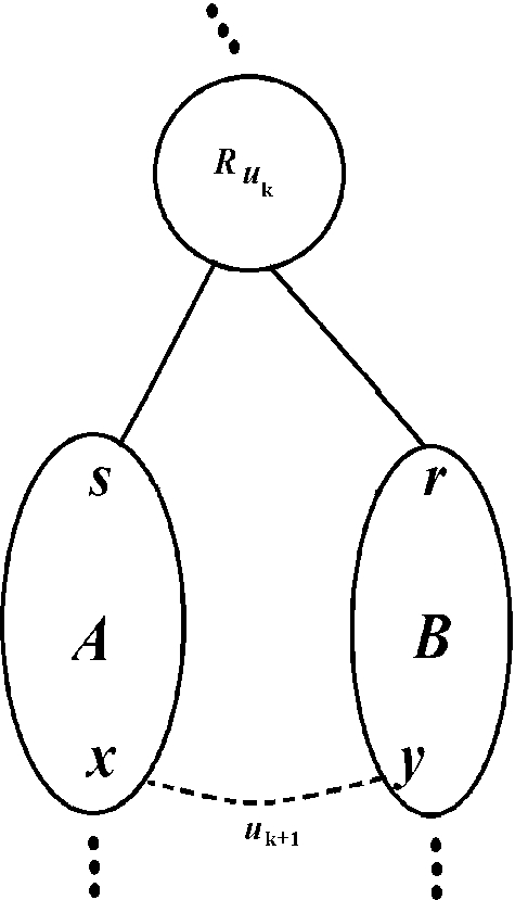
  Since $u_{k+1}$ is the edge of rank k for the ordering $\prec '$, we can say that the k-partition $\mathbf{B }'_k$ by the ordering $\prec '$ is $\{A \cup B\} \cup (\mathbf{B }'_{k-1} {\setminus } \{A,B\})$ because A and B are the regions of $\mathbf{B }'_{k-1}$ that contain, respectively, x and y. As the region $\{A \cup B\}$ does not belong to the partition $\mathbf{B }'_{k-1}$, we have that $u_{k+1}$ is the building edge of the region $\{A \cup B\}$. Hence, $u_{k+1}$ is a building edge for $\prec '$.

  Since $u_{k}$ is the edge of rank $k+1$ for the ordering $\prec '$, we may conclude that $\mathbf{B }'_{k+1} = \mathbf{B }'_{k}$ because the s and r belong to the same region $\{A \cup B\}$ of $\mathbf{B }'_{k}$. Therefore, $u_k$ is not a building edge for $\prec '$. This situation is illustrated in the following image.

  

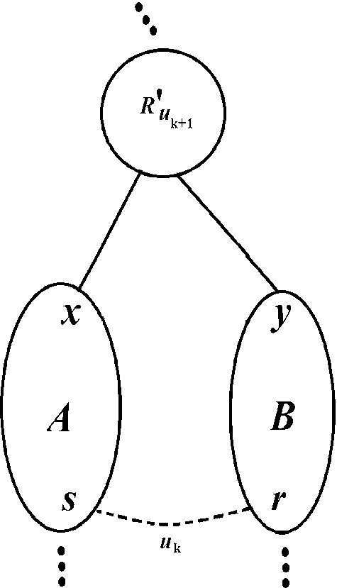
  We conclude that ${\mathcal {B}}_\prec$ and ${\mathcal {B}}_{\prec '}$ have the same set of regions but not the same set of building edges: $E_{\prec '} = E_\prec {\setminus }\{u_{k}\} \cup \{u_{k+1}\}$. Hence, the only difference between the hierarchies ${\mathcal {B}}_\prec$ and ${\mathcal {B}}_{\prec '}$ is the building edge of the region $\{A \cup B\}$. Therefore, we may say that, if the weight of the building edge of $\{A \cup B\}$ for $\prec$ is equal to the weight of the building edge of $\{A \cup B\}$ for $\prec '$, then f is also one-side increasing for $\prec '$. To that end, we will prove that $f(u_k) = f(u_{k+1})$.

  By Lemma 22, as f is one-side increasing for $\prec$, we have that:

  • III. $(V,E_\prec )$ is a MST of (G, f)

  By the statement III and by Lemma 21, we conclude that:

  • IV. the hierarchy $\mathcal {QFZ}(G,f)$ is equal to the hierarchy $\mathcal {QFZ}((V,E_\prec ),f)$

  Statement IV implies that f is the saliency map of the hierarchy $\mathcal {QFZ}((V,E_\prec ),f)$. Hence, for any edge $u=\{a,b\}$ in E, f(u) is the maximum weight in the unique path between a and b in $((V,E_\prec ),f)$. We can affirm that:

  • V. the unique path between x and y in $((V,E_\prec ),f)$ is a path that includes the edge $u_{k}$

  By the statement V and by the definition of saliency maps, we have $f(u_{k+1}) \ge f(u_{k})$. Since k is a critical rank for f and $\prec$, we have $f(u_{k+1}) \le f(u_{k})$. Therefore, we have $f(u_k) = f(u_{k+1})$, which completes the proof that f is one-side increasing for $\prec '$.$\square$

Proof of Property 6

Property 6

Let $\prec$ be an altitude ordering for w and let $\epsilon$ be a map from the regions of ${\mathcal {B}}_{\prec }$ into $\mathbb {R}$. The map $\epsilon$ is an extinction map for $\prec$ if and only if the following statements hold true:

• $\{\epsilon (R) \mid R$ is a region of ${\mathcal {B}}_{\prec }\} = \{0, \ldots , n \}$;

• for any two distinct minima $M_1$ and $M_2$ of w, we have $\epsilon (M_1) \ne \epsilon (M_2)$; and

• for any region R of ${\mathcal {B}}_{\prec }$, we have that $\epsilon (R)$ is equal to $\vee \{\epsilon (M)$ such that M is a minimum of w included in $R\}$, where $\vee \{\}=0$.

We prove the forward and backward implications of Property 6 in Lemmas 35 and 36, respectively.

Lemma 35

Let $\prec$ be an altitude ordering for w and let $\epsilon$ be a map from the regions of ${\mathcal {B}}_{\prec }$ into $\mathbb {R}$. If the map $\epsilon$ is an extinction map for $\prec$, then the following statements hold true:

• 1. $\{\epsilon (R) \mid R$ is a region of ${\mathcal {B}}_{\prec }\} = \{0, \ldots , n \}$;

• 2. for any two distinct minima $M_1$ and $M_2$ of w, we have $\epsilon (M_1) \ne \epsilon (M_2)$; and

• 3. for any region R of ${\mathcal {B}}_{\prec }$, we have that $\epsilon (R)$ is equal to $\vee \{\epsilon (M)$ such that M is a minimum of w included in $R\}$, where $\vee \{\}=0$.

Proof

Let $\epsilon$ be an extinction map for $\prec$. Then, by the definition of extinction maps, there is a sequence ${\mathcal {S}}=(M_1, \ldots , M_n)$ of minima of w such that $\epsilon$ is the extinction map for $\prec$ and ${\mathcal {S}}$. We will prove that the statements 1, 2 and 3 hold true for $\epsilon$.

To prove that the statement 1 holds true, we will first prove that $\{\epsilon (R) \mid R$ is a region of ${\mathcal {B}}_{\prec }\} \subseteq \{0, \ldots , n \}$. Since w has n minima, the extinction value of any region of ${\mathcal {B}}_{\prec }$ which includes a minimum of w is in the set $\{1, \ldots , n\}$. On the other hand, for any region R of ${\mathcal {B}}_{\prec }$ which do not include any minimum of w, we have that $\epsilon (R) = 0$. Hence, $\{\epsilon (R) \mid R$ is a region of ${\mathcal {B}}_{\prec }\} \subseteq \{0, \ldots , n \}$. We will now prove that $\{0, \ldots , n \} \subseteq \{\epsilon (R) \mid R$ is a region of ${\mathcal {B}}_{\prec }\}$. As ${\mathcal {B}}_\prec$ has at least one leaf region composed of a single vertex of G, we can affirm that there is at least one region of ${\mathcal {B}}_\prec$ which do not include any minimum of w and whose extinction value for $\prec$ and ${\mathcal {S}}$ is zero. Then, 0 is in $\{\epsilon (R) \mid R$ is a region of ${\mathcal {B}}_{\prec }\}$. Now, let i be a value in $\{1, \ldots , n \}$. For the minimum $M_i$, we may affirm that $M_i$ is the unique minimum of w included in $M_i$ and, therefore, $\epsilon (M_i) = i$. Hence, i is in $\{\epsilon (R) \mid R$ is a region of ${\mathcal {B}}_{\prec }\}$. We may conclude that, for any i in $\{0, \ldots , n \}$, i is in $\{\epsilon (R) \mid R$ is a region of ${\mathcal {B}}_{\prec }\}$. Therefore, the range of $\epsilon$ is $\{0, \ldots , n\}$, which corresponds to the statement 1 of Lemma 35.

By the definition of extinction maps, for any minimum $M_i$, for i in $\{1, \ldots , n\}$, we have $\epsilon (M_i) = i$ because $M_i$ is the only minimum of w included in $M_i$. Therefore, for any two distinct minima $M_i$ and $M_j$, for i, j in $\{1, \ldots , n\}$, we have $\epsilon (M_i) = i$ and $\epsilon (M_j) = j$ and, consequently, $\epsilon (M_i)$ is different from $\epsilon (M_j)$. Hence, the statement 2 of Lemma 35 holds true for $\epsilon$.

The statement 3 of Lemma 35 is precisely the definition of extinction values: for any region R of ${\mathcal {B}}_{\prec }$, the extinction value of R is zero if there is no minimum of w included in R and, otherwise, it is the maximal i (which is equal to $\epsilon (M_i)$) such that $M_i$ is included in R. $\square$

Lemma 36

Let $\prec$ be an altitude ordering for w and let $\epsilon$ be a map from the regions of ${\mathcal {B}}_{\prec }$ into $\mathbb {R}$ such that:

• 1. $\{\epsilon (R) \mid R$ is a region of ${\mathcal {B}}_{\prec }\} = \{0, \ldots , n \}$;

• 2. for any two distinct minima $M_1$ and $M_2$ of w, we have $\epsilon (M_1) \ne \epsilon (M_2)$; and

• 3. for any region R of ${\mathcal {B}}_{\prec }$, we have that $\epsilon (R)$ is equal to $\vee \{\epsilon (M)$ such that M is a minimum of w included in $R\}$, where $\vee \{\}=0$.

Then, the map $\epsilon$ is an extinction map for $\prec$.

Proof

To prove that $\epsilon$ is an extinction map for $\prec$, we will show that there exists a sequence $S=(M_1, \ldots , M_n)$ of minima of w such that, for any region R of ${\mathcal {B}}_{\prec }$, the value $\epsilon (R)$ is the extinction value of R for $\prec$ and ${\mathcal {S}}$.

Let ${\mathcal {S}} = (M_1, \ldots , M_n)$ be a sequence of minima of w ordered in non-decreasing order for $\epsilon$, i.e. for any two distinct minima $M_i$ and $M_j$, with i, j in $\{1, \ldots , n\}$, if $\epsilon (M_i) <\epsilon (M_j)$ then $i < j$.

By the hypothesis 2, this sequence ${\mathcal {S}}$ is unique. By the hypothesis 3, for any region R of ${\mathcal {B}}$ such that there is no minimum of w included in R, $\epsilon (R) = \vee \{\} = 0$, so $\epsilon (R)$ is the extinction value of R for $\prec$ and ${\mathcal {S}}$.

Since w has n minima, for any minimum M of w, the value $\epsilon (M)$ is in $\{1, \ldots , n\}$. Otherwise, by contradiction, let us assume that there exists a minimum $M'$ of w such that $\epsilon (M') = 0$. Then, there is a value i in $\{1, \ldots , n\}$ such that, for any minimum $M''$ of w, the value $\epsilon (M'')$ is different from i. Consequently, by the hypothesis 3, the range of $\epsilon$ would be $\{0, \ldots , n\} {\setminus } \{i\}$, which contradicts the hypothesis 1. Therefore, for any minimum $M_i$ of w, for i in $\{1, \ldots , n\}$, as our assumption that $\epsilon (M_i) <\epsilon (M_j)$ implies that $i < j$, we have that $\epsilon (M_i) = i$. Thus, $\epsilon (M_i)$ is the extinction value of $M_i$ for $\prec$ and S.

It follows that, by the hypothesis 3, for any region R of ${\mathcal {B}}_{\prec }$ such that there is a minimum of w included in R, the value $\epsilon (R)$ is the maximum value i (which is equal to $\epsilon (M_i)$) in $\{1, \ldots , n\}$ such that $M_i$ is included in R.

Thus, for any region R of ${\mathcal {B}}_{\prec }$, the value $\epsilon (R)$ is the extinction value of R for $\prec$ and ${\mathcal {S}}$. Therefore, the map $\epsilon$ is an extinction map for $\prec$. $\square$

Proof of Lemma 11

Lemma 11

Let $\prec$ be an altitude ordering for w, let f be a map from E into $\mathbb {R}$ such that f is one-side increasing for $\prec$, and let $\xi$ be the approximated extinction map for f and $\prec$. The map $\xi$ is an extinction map for $\prec$.

In order to prove Lemma 11, we prove in Lemmas 38, 39 and 43 that the three conditions of Property 6 for $\xi$ to be an extinction map are satisfied. We first establish the following auxiliary lemma.

Lemma 37

Let $\prec$ be an altitude ordering for w and let f be a map from E into $\mathbb {R}$ such that f is one-side increasing for $\prec$. Then, the two following statements hold true:

• 1. the set $\{f(e) \mid e\ is\ a\ watershed-cut\ edge\ for\ \prec \}$ is equal to $\{1, \ldots , n-1\}$; and

• 2. for any two distinct watershed-cut edges u and v for ${\mathcal {B}}$, we have $f(u) \ne f(v)$.

Proof

By Definition 3 (statement 1), we have $\{f(u) \mid u \in E_\prec \}=\{0, \ldots , n-1\}$ and, by Definition 3 (statement 2), only the weight of the watershed-cut edges for $\prec$ are strictly greater than zero. Then, $\{f(e) \mid e\ is\ a\ watershed-cut\ edge\ for\ \prec \} = \{1, \ldots , n-1\}$. Hence, for any i in $\{1, \ldots , n-1\}$, there is a watershed-cut edge e for $\prec$ such that $f(e) = i$. Moreover, as there are $n-1$ watershed-cut edges for $\prec$, for any two distinct watershed-cut edges u and v for $\prec$, we have $f(u) \ne f(v)$. $\square$

Lemma 38

Let $\prec$ be an altitude ordering for w, let f be a map from E into $\mathbb {R}$ such that f is one-side increasing for $\prec$, and let $\xi$ be the approximated extinction map for f and $\prec$. The range of $\xi$ is $\{0,\ldots ,n\}$.

Proof

We will prove that: (1) for any i in $\{0, \ldots , n\}$, there is a region R of ${\mathcal {B}}_{\prec }$ such that $\xi (R) = i$; and (2) for any region R of ${\mathcal {B}}_{\prec }$, we have $\xi (R)$ in $\{0, \ldots , n\}$.

• (1) We first prove statement (1). We start by proving that there is a region R of ${\mathcal {B}}_{\prec }$ such that $\xi (R) = n$. Let R be the set V of vertices of G. Then, by Definition 10 (statement 1), we have $\xi (R) = \bigtriangledown (R)+1$, where $\bigtriangledown$ is the supremum descendant map for f and $\prec$. By Definition 3 (statement 1), we have $\{f(u) \mid u \in E_\prec \}=\{0, \ldots , n-1\}$. As $\bigtriangledown (V) = \vee \{f(u) \mid R_u \subseteq V\} = \vee \{0, \ldots , n-1\}= n-1$, we have that $\xi (R) = n-1+1 = n$.

  We will now show that there is a region R of ${\mathcal {B}}_{\prec }$ such that $\xi (R) = 0$. Let R be a region of ${\mathcal {B}}_\prec$ such that there is no minimum of w included in R. Then, R is not a minimum of w and, consequently, the building edge of the parent of R is not a watershed-cut edge for $\prec$. Let u be building edge of the parent of R. Since there is no minimum of w included in R, by Definition 9, R is not a dominant region for f and $\prec$. By the statement 3 of the definition of approximated extinction maps (Definition 10), we have $\xi (R)=f(u)$. Since f is a one-side increasing map and since u is not a watershed-cut edge for $\prec$, we have $f(u) = 0$. Therefore, we have $\xi (R) = f(u) = 0$.

  Finally, we will prove that, for any i in $\{1, \ldots , n-1\}$, there is a region R of ${\mathcal {B}}_\prec$ such that $\xi (R) = i$. By Lemma 37, we can say that, for any i in $\{1, \ldots , n-1\}$, there is a watershed-cut u edge for $\prec$ such that $f(u)=i$. Let u be a watershed-cut edge for $\prec$ and let X and Y be the children of $R_u$. Since u is a watershed-cut edge for $\prec$, both X and Y contain at least a minimum of w and, then, neither X nor Y are leaf regions of ${\mathcal {B}}_\prec$. Let $\ll$ be the non-leaf ordering for f and $\prec$. Since $\ll$ is a total ordering, we have either $X \ll Y$ or $Y \ll X$. Then, exactly one child of $R_u$ is a dominant region for f and $\prec$. Let Y (resp. X) be the child of $R_u$ which is not a dominant region for f and $\prec$. By Definition 10 (statement 3), we have $\xi (Y) = f(u)$ (resp. $\xi (X) = f(u)$). Therefore, for any i in $\{1, \ldots , n-1\}$, there is a watershed-cut edge u for $\prec$ such that $f(u) = i$ and such that there is a child Z of $R_u$ such that $\xi (Z) = i$.

• (2) We will now prove the statement 2. Let R be a region of ${\mathcal {B}}_{\prec }$. If $R= V$, then $\xi (R) = n$, as established in the proof of statement 1. Otherwise, let v be the building edge of the parent of R. By Definition 10, the value $\xi _f(R)$ is either f(v) or $\xi (parent(R))$. Hence, either $\xi _f(R)$ is equal to f(v) for a building edge v for $\prec$, or $\xi _f(R)$ is equal to $\xi (V) = n$. It is enough to prove that n and f(v) are in $\{0, \ldots , n\}$. As f is one-side increasing for $\prec$, by Definition 3 (statement 1), we have $\{f(u) \mid u \in E_\prec \} = \{0, \ldots , n-1\}$. Since v is a building edge for $\prec$, we may say that f(v) is in $\{0, \ldots , n-1\}$.$\square$

Lemma 39

Let $\prec$ be an altitude ordering for w and let f be a map from E into $\mathbb {R}$ such that f is one-side increasing for $\prec$. Let $\xi$ be the approximated extinction map for f and $\prec$. For any two minima $M_1$ and $M_2$ of w, if $\xi (M_1) = \xi (M_2)$, then $M_1 = M_2$.

To prove Lemma 39, we first present the Lemmas 40, 41 and 42 . In the following, for any non-leaf region X of a binary partition hierarchy ${\mathcal {B}}$ of (G, w), we denote by $u_X$ the building edge of X.

Lemma 40

Let $\prec$ be an altitude ordering for w and let f be a map from E into $\mathbb {R}$ such that f is one-side increasing for $\prec$. Let $\xi$ be the approximated extinction map for f and $\prec$. For any region X of ${\mathcal {B}}_{\prec }$ such that there is a minimum M of w such that $M \subset X$, there is a child Y of X such that:

• 1. $\xi (Y) = \xi (X)$;

• 2. $\xi (sibling(Y)) = f(u_X)$; and

• 3. there is a minimum of w included in Y.

Proof

Let X be a region such that there is a minimum M of w such that $M \subset X$. Then, there is a child Z of X such that there is a minimum M such that $M \subseteq Z$. Let Z be a child X such that there is a minimum M such that $M \subseteq Z$. We consider two cases: (1) sibling(Z) is a leaf region of ${\mathcal {B}}_\prec$; and (2) sibling(Z) is a non-leaf region of ${\mathcal {B}}_\prec$.

• (1) If sibling(Z) is a leaf region of ${\mathcal {B}}_\prec$, then, by Definition 9, Z is a dominant region for f and $\prec$ and sibling(Z) is not a dominant region for f and $\prec$. Hence, by Definition 10, $\xi (Z) = \xi (X)$ and $\xi (sibling(Z)) = f(u_X)$.

• (2) Let us now assume that sibling(Z) is a non-leaf region of ${\mathcal {B}}_\prec$. Since X is not a minimum of w and since there is a minimum of w included in Z, we can conclude that there is a minimum of w included in sibling(Z) as well. Let $\ll$ be the non-leaf ordering for f and $\prec$. As the non-leaf ordering $\ll$ is a total ordering on the non-leaf regions of ${\mathcal {B}}_\prec$, we have either $Z \ll sibling(Z)$ or $sibling(Z) \ll Z$. Then, by the definition of dominant regions (Definition 9), we have that either Z or sibling(Z) is a dominant region for f and $\prec$. Let us assume that Z is a dominant region for f and $\prec$. Then, by Definition 10, we have $\xi (Z) = \xi (X)$ and $\xi (sibling(Z)) = f(u_X)$. Otherwise, if sibling(Z) is a dominant region for f and $\prec$, we have $\xi (sibling(Z)) = \xi (X)$ and $\xi (Z) = f(u_X)$. Since both Z and sibling(Z) include at least one minimum of w, we may say that there is a child Y of X for which the hypothesis 1, 2 and 3 hold true.$\square$

Lemma 41

Let $\prec$ be an altitude ordering for w and let f be a map from E into $\mathbb {R}$ such that f is one-side increasing for $\prec$. Let $\xi$ be the approximated extinction map for f and $\prec$. Let u be a watershed-cut edge for $\prec$. Then, there is a minimum M of w such that $\xi (M) = f(u)$.

Proof

As u is a watershed-cut edge for $\prec$, each child of $R_u$ includes at least one minimum of w. Then, there is a minimum M of w such that $M \subset R_u$. By Lemma 40, there is a child $Y_1$ of $R_u$ such that $\xi (Y_1) = f(u)$. If $Y_1$ is a minimum of w, then the property holds true. Otherwise, if $Y_1$ is not a minimum of w, it means that there is a minimum M of w such that $M \subset Y_1$. By Lemma 40, there is a child $Y_2$ of $Y_1$ such that $\xi (Y_2) = \xi (Y_1) = f(u)$ and such that there is a minimum of w included in $Y_2$. Again, if $Y_2$ is a minimum of w, then the property holds true. Otherwise, we can apply this same reasoning indefinitely. We can define a sequence $(Y_1, \ldots , Y_p)$ of regions of ${\mathcal {B}}_\prec$ where $Y_p$ is a minimum of w and such that $\xi (Y_p) = \ldots = \xi (Y_1) = f(u)$ and $Y_i \subset Y_{i-1}$ for any i in $\{2, \ldots , p\}$. Therefore, there is a minimum $Y_p$ included in $R_u$ such that $\xi (Y_p) = f(u)$. $\square$

Lemma 42

Let $\prec$ be an altitude ordering for w and let f be a map from E into $\mathbb {R}$ such that f is one-side increasing for $\prec$. Let $\xi$ be the approximated extinction map for f and $\prec$. Let X be a region of ${\mathcal {B}}_\prec$ such that X contains at least one minimum of w. There exists a minimum $M \subseteq X$ such that $\xi (M) = \xi (X)$.

Proof

If X is a minimum of w, then it is trivial. Otherwise, by Lemma 40, there is a child $Y_1$ of X such that $\xi (Y_1) = \xi (X)$ and such that there is a minimum of w included in $Y_1$. If $Y_1$ is a minimum of w, then the property holds true. Otherwise, by Lemma 40, there is a child $Y_2$ of $Y_1$ such that $\xi (Y_2) = \xi (Y_1) = \xi (X)$ and such that there is a minimum of w included in $Y_2$. Again, if $Y_2$ is a minimum of w, then the property holds true. Otherwise, we can apply this same reasoning indefinitely. We can define a sequence $(Y_1, \ldots , Y_p)$ of regions of ${\mathcal {B}}_\prec$ where $Y_p$ is a minimum of w and such that $\xi (Y_p) = \ldots = \xi (Y_1) = \xi (X)$ and $Y_i \subset Y_{i-1}$ for any i in $\{2, \ldots , p\}$. Therefore, there is a minimum $Y_p$ included in X such that $\xi (Y_p) = \xi (Y)$. $\square$

Proof of Lemma 39

In order to prove that

• (1) for any two minima $M_1$ and $M_2$ of w, if $\xi (M_1) = \xi (M_2)$, then $M_1 = M_2$,

we will prove that

• (2) for any two minima $M_1$ and $M_2$ of w, we have $\xi (M_1) \ne \xi (M_2)$.

As w has n minima, it suffices to prove that, for any i in $\{1, \ldots , n\}$, there is a minimum M of w such that $\xi (M)=i$.

By Lemma 41, for any watershed-cut edge u for ${\mathcal {B}}_{\prec }$, there is a minimum M such that $\xi (M) = f(u)$. By Lemma 37, for any i in $\{1, \ldots , n-1\}$, there is a watershed-cut edge such that $f(u)=i$. Then, for any i in $\{1,\ldots , n-1\}$, there is a minimum M of w such that $\xi (M)=i$.

Since, f is one-side increasing for $\prec$, we have $\vee \{f(v) \mid R_v \in V\} = \{0,\ldots ,n-1\}$. Then, we can conclude that $\xi (V) = \vee \{f(v) \mid R_v \in V\} + 1 = (n-1)+1= n$. By Lemma 42, there is a minimum M of w such that $\xi (M) = \xi (V) = n$.

Therefore, for any i in $\{1,\ldots , n\}$, there is a minimum M of w such that $\xi (M)=i$. Since w has n minima, it implies that the values $\xi (M_1)$ and $\xi (M_2)$ are distinct for any pair $(M_1, M_2)$ of distinct minima of w. Hence, for any two minima $M_1$ and $M_2$ of w, if $\xi (M_1) = \xi (M_2)$, then $M_1 = M_2$. $\square$

Lemma 43

Let $\prec$ be an altitude ordering for w and let f be a map from E into $\mathbb {R}$ such that f is one-side increasing for $\prec$. Let $\xi$ be the approximated extinction map for f and $\prec$. For any region R of ${\mathcal {B}}_\prec$, we have $\xi _f(R) = \vee \{\xi _f(M)$ such that M is a minimum of w included in $R\}$.

To prove Lemma 43, we introduce Lemma 44.

Lemma 44

Let $\prec$ be an altitude ordering for w and let f be a map from E into $\mathbb {R}$ such that f is one-side increasing for $\prec$. Let $\xi$ be the approximated extinction map for f and $\prec$. Let $\bigtriangledown$ be the supremum descendant map for f and $\prec$. Let X be a region of ${\mathcal {B}}_\prec$. Then, $\xi (X)$ is greater than or equal to the supremum descendant value $\bigtriangledown (X)$ of X.

Proof

We consider the following cases: (1) $X=V$, (2) $X \ne V$ and X is not a dominant region for f and $\prec$; and (3) X is a dominant region for f and $\prec$. Let $\ll$ be the non-leaf ordering for f and $\prec$.

• 1. If $X = V$, then $\xi (X) = \xi (V) = \bigtriangledown (V)+1$ (first case of Definition 10). Then, $\xi (X)$ is clearly than $\bigtriangledown (X)$.

• 2. If $X\ne V$ and if X is not a dominant region for f and $\prec$, then $\xi (X) = f(u)$ (third case of Definition 10), where u is the building edge of the parent of X. By the definition of dominant regions, we consider two cases: (a) there is no minimum M of w such that $M \subseteq X$; or (b) $X \ll sibling(X)$.

  • (a) If there is no minimum M of w such that $M \subseteq X$, then there is no descendant of X whose building edge is a watershed-cut edge for $\prec$. Hence, for any edge v such that $R_v \subseteq X$, u is not a watershed-cut edge for $\prec$ and, since f is one-side increasing for $\prec$, we have $f(v)=0$ Definition 3 (statement 2). Therefore, $\bigtriangledown (X)=0$. By Definition 3 (statement 1), we have $\{f(v) \mid v \in E_\prec \}=\{0, \ldots , n-1\}$. Hence, $\xi (X)$, being equal to f(u), is greater than or equal to $\bigtriangledown (X)=0$.

  • (b) If $X \ll sibling(X)$, then, by the definition of non-leaf ordering, we have:

    • (i) either $\bigtriangledown (X) < \bigtriangledown (sibling(X))$; or

    • (ii) $\bigtriangledown (X) = \bigtriangledown (sibling(X))$ and $u_X \prec u_{sibling(X)}$.

    Thus, we have $\bigtriangledown (X) \le \bigtriangledown (sibling(X))$. Since f is one-side increasing for $\prec$, by the statement 3 of Definition 3, there is a child Y of parent(X) such that $f(u) \ge \vee \{f(v) \mid R_v \subseteq Y\}$. Hence, there is a child Y of parent(X) such that $f(u) \ge \bigtriangledown (Y)$. Then, we have $f(u) \ge \bigtriangledown (X)$ or $f(u) \ge \bigtriangledown (sibling(X))$. In the case where $f(u) \ge \bigtriangledown (sibling(X))$, this also implies that $f(u) \ge \bigtriangledown (X)$ because $\bigtriangledown (X) \le \bigtriangledown (sibling(X))$. Therefore, $\xi (X)$, being equal to f(u), is greater than or equal to $\bigtriangledown (X)$.

• 3. If X is a dominant region for f and $\prec$, then $\xi (X) = \xi (parent(X))$ (second case of Definition 10). We will prove by induction that this lemma holds true for any dominant region for f and $\prec$. In the base step, we consider that parent(X) is V. In the inductive step, we show that, if the property holds true for parent(X), then it also holds true for X. Please note that, if parent(X) is not a dominant region for f and $\prec$, the property holds for parent(X) as proven in the previous case.

  • (a) Base step: if parent(X) is V, then $\xi (X) = \xi (V) = \bigtriangledown (V)+1$ (first case of Definition 10). We can see that $\bigtriangledown (V) \ge \bigtriangledown (X)$ because, for any edge u such that $R_u \subseteq X$, we also have $R_u \subseteq V$. Then, $\xi (X)$, being equal to $\bigtriangledown (V)+1$, is greater than $\bigtriangledown (X)$.

  • (b) Inductive step: let us assume that $\xi (parent(X)) \ge \bigtriangledown (parent(X))$. Since $\xi (X) = \xi (parent(X))$, we have $\xi (X) \ge \bigtriangledown (parent(X))$. We can affirm that, for any edge v in $E_\prec$ such that $R_v \subseteq X$, we also have $R_v \subseteq parent(X)$. Hence, $\bigtriangledown (parent(X)) \ge \bigtriangledown (X)$. Therefore, $\xi (X)$, being equal to $\xi (parent(X))$, is greater than or equal to $\bigtriangledown (X)$. $\square$

Proof of Lemma 43

We will prove that, for any region X of ${\mathcal {B}}_\prec$, we have $\xi (X) = \vee \{\xi _f(M)$ such that M is a minimum of w included in $X\}$. Let X be a region of ${\mathcal {B}}_\prec$. We consider two cases: (1) there is a minimum of w included in X; and (2) there is no minimum of w included in X.

• (1) If there is no minimum of w included in X, then X is not a dominant region for f and $\prec$. Then, $\xi (X) = f(u)$ (third condition of Definition 10), where u is the building edge of parent(X). The edge u is not a watershed-cut edge for $\prec$ because the child X of $R_u$ does not include any minimum of w. Hence, since f is one-side increasing for $\prec$, by the statement 2 of Definition 3, we have $f(u)=0$. Therefore, $\xi (X)$, being equal to f(u), is also equal to $\vee \{\xi (M)$ such that M is a minimum of w included in $R\} = \vee \{\} = 0$.

• (2) Let us assume that there is at least one minimum of w included in X. If X is a minimum of w, then $\xi (X) = \vee \{\xi _f(M)$ such that M is a minimum of w included in $X\}=\vee \{\xi _f(X)\}$.

  In order to prove the case where X is not a minimum of w, we will first demonstrate that $\xi (X) \ge \vee \{\xi (Y) \mid Y \subseteq X\}$.

  To prove that $\xi (X) \ge \vee \{\xi (Y) \mid Y \subseteq X\}$, it is enough to demonstrate that, for any region Z of ${\mathcal {B}}_\prec$, we have $\xi (Z) \ge \vee \{\xi (Y) \mid Y\ is\ a\ child\ of\ Z\}$. Let Z be a region of ${\mathcal {B}}_\prec$. If Z is a leaf region of ${\mathcal {B}}_\prec$, then $\xi (Z) \ge \vee \{\xi (Y) \mid Y\ is\ a\ child\ of\ Z\}=\vee \{\}=0$ because, by Lemma 38, $\xi (Z)$ is in $\{0, \ldots , n\}$. Let us now assume that Z is not a leaf region of ${\mathcal {B}}_\prec$ and let Y be a child of Z. If Y is a dominant region for f and $\prec$, then $\xi (Y)=\xi (Z)$ and, consequently, $\xi (Z) \ge \xi (Y)$. Otherwise, if Y is not a dominant region for f and $\prec$, then $\xi (Y)=f(v)$, where v is the building edge of Z. By Lemma 44, $\xi (Z) \ge \bigtriangledown (Z)$ and, consequently, $\xi (Z) \ge f(u)$. Hence, $\xi (Z) \ge \xi (Y)$.

  We can now prove that $\xi (X) = \vee \{\xi _f(M)$ such that M is a minimum of w included in $X\}$ in the case where X is not a minimum of w. By Lemma 42, there is a minimum M of w such that $M \subset X$ and such that $\xi (M) = \xi (X)$. Let M be the minimum of w such that $\xi (M) = \xi (X)$. Since $\xi (X) \ge \vee \{\xi (Y) \mid Y \subseteq X\}$, we can say that $\xi (X) = \vee \{\xi _f(M')$ such that $M'$ is a minimum of w included in $X\}$.$\square$

Proof of Lemma 12

Lemma 12

Let $\prec$ be an altitude ordering for w and let f be a map from E into $\mathbb {R}$ such that f is one-side increasing for ${\mathcal {B}}_{\prec }$. Then, for any u in $E_\prec$, we have:

$$\begin{aligned} f(u) = min\{\xi (R) \text { such that } R \text { is a child of } R_u\}. \end{aligned}$$

Proof

Let u be an edge in $E_\prec$. By the definition of dominant regions, we have that at most one child of $R_u$ is a dominant region for f and $\prec$. Therefore, there is a child of $R_u$ which is not a dominant region for f and $\prec$. Let X be the child of $R_u$ which is not a dominant region for f and $\prec$. Then, $\xi (X) = f(u)$ (by the third condition of Definition 10). If sibling(X) is not a dominant region for f and $\prec$, then $\xi (sibling(X)) = f(u)$ as well and, consequently, $f(u) = min\{\xi (R)$ such that R is a child of $R_u\}= min\{f(u),f(u)\}$. Otherwise, let us assume that sibling(X) is a dominant region for f and $\prec$. Then, $\xi (sibling(X)) = \xi (R_u)$. By Lemma 44, we can infer that $\xi (R_u) \ge f(u)$. Therefore, $min\{\xi (Y)$ such that Y is a child of $R_u\} = min\{\xi _f(X), \xi (sibling(X))\} = min\{f(u), \xi (R_u)\} = f(u)$. $\square$

Proof of Lemma 4

Lemma 4

Let ${\mathcal {H}}$ be a hierarchy on V. The hierarchy ${\mathcal {H}}$ is a hierarchical watershed of (G, w) if and only if there is an altitude ordering $\prec$ for w such that $\varPhi ({\mathcal {H}})$ is one-side increasing for $\prec$.

Proof

We prove the forward and backward implications of Lemma 4 in Lemmas 45 and 46, respectively. $\square$

Lemma 45

Let ${\mathcal {H}}$ be a hierarchy on V. If the hierarchy ${\mathcal {H}}$ is a hierarchical watershed of (G, w), then there exists an altitude ordering $\prec$ for w such that $\varPhi ({\mathcal {H}})$ is one-side increasing for $\prec$.

Proof

By Lemma 16, there is a sequence of minima ${\mathcal {S}}$ of w such that ${\mathcal {H}}$ is the hierarchy induced by $\prec$ and ${\mathcal {S}}$. In order to prove that $\varPhi ({\mathcal {H}})$ is one-side increasing for $\prec$, by Definition 3, we will prove that the following three statements hold true:

• 1. $\{\varPhi ({\mathcal {H}})(e) \mid e \in E_\prec \} = \{0, \ldots , n-1\}$;

• 3. for any edge u in $E_\prec$, $\varPhi ({\mathcal {H}})(u) > 0$ if and only if u is a watershed-cut edge for $\prec$; and

• 4. for any edge u in $E_\prec$, there exists a child R of $R_u$ such that $\varPhi ({\mathcal {H}})(u) \ge \vee \{ \varPhi ({\mathcal {H}})(v)$ such that $R_v$ is included in $R\}$, where $\vee \{\} = 0$.

In the remainder of this proof, let $\rho$ and $\epsilon$ be, respectively, the persistence map and the extinction map for $\prec$ and ${\mathcal {S}}$.

• 1. By Lemma 20, we have $\{\varPhi ({\mathcal {H}})(e) \mid e \in E_\prec \} = \{\rho (e) \mid e \in E_\prec \}$. Then, as Lemma 19 states that the range of $\rho$ is $\{0, \ldots , n-1\}$, we can conclude that $\{\varPhi ({\mathcal {H}})(e) \mid e \in E_\prec \}$ is the set $\{0, \ldots , n-1\}$.

• 2. Let u be a building edge for $\prec$. Given the following propositions:

  • (a) u is a watershed-cut edge

  • (b) $\varPhi ({\mathcal {H}})(u) > 0$

  we will prove that (a) implies (b), and that not (b) implies not (a).

  If u is a watershed-cut edge for $\prec$, then both children of $R_u$ contain at least one minimum of w. Therefore, the extinction value of both children of $R_u$ is nonzero and, consequently, the persistence value $\rho (u)$ of u is nonzero. Moreover, by Lemma 20, in this case we have $\varPhi ({\mathcal {H}})(e)=\rho (e)$ for any building edge e for $\prec$. Thus, $\varPhi ({\mathcal {H}})(u)$ is nonzero.

  On the other hand, if u is not a watershed-cut edge for $\prec$, then there is a child X of $R_u$ which does not contain any minimum of w. Therefore, the extinction value of X is equal to 0: $\epsilon (X)=0$. Since, by definition $\rho (u) = min\{\epsilon (X), \epsilon (sibling(X))\}$ and the minimal extinction value is zero, we can say that $\rho (u) = 0$. Again, by Lemma 20, in this case we have $\varPhi ({\mathcal {H}})(e)=\rho (e)$ for any building edge e for $\prec$ and thus, $\varPhi ({\mathcal {H}})(u)$ is equal to 0.

• 3. Let u be a building edge for $\prec$. The persistence value of u is the extinction value of a child X of $R_u$. Let X be a child of $R_u$ such that $\rho (u)$, the persistence value of u, is equal to $\epsilon (X)$, the extinction value of X. By Lemma 17, for any region Y of ${\mathcal {B}}_\prec$ such that $Y \subseteq X$ , we have $\epsilon (Y) \le \epsilon (X)$ and, as $X\subseteq R_u$, $\epsilon (Y) \le \epsilon (R_u)$. Let v be the building edge of a region $Z \subseteq X$. Then, we can say that the extinction value of both children of Z is less than or equal to the extinction value $\epsilon (X)$. Hence, $\rho (v) \le \epsilon (X)$ and, then, $\rho (v) \le \rho (u)$. By Lemma 20, we can conclude that $\varPhi ({\mathcal {H}})(v) \le \varPhi ({\mathcal {H}})(u)$. Hence, $\varPhi ({\mathcal {H}})(u) \ge \vee \{ \varPhi ({\mathcal {H}})(v)$ such that $R_v$ is included in $X\}$. $\square$

Lemma 46

Let ${\mathcal {H}}$ be a hierarchy on V and let $\prec$ be an altitude ordering such that $\varPhi ({\mathcal {H}})$ is one-side increasing for $\prec$. Then, the hierarchy ${\mathcal {H}}$ is a hierarchical watershed of (G, w).

Proof

Let $\xi$ be the approximated extinction map for $\varPhi ({\mathcal {H}})$ and $\prec$. By Lemma 12, for any edge in $E_\prec$, we have  $\varPhi ({\mathcal {H}})(u) = min\{\xi (R)$ such that R is a child of $R_u\}$. By Lemma 11, the map $\xi$ is an extinction map for $\prec$. Then, by the backward implication of Property 7, the hierarchy ${\mathcal {H}}$ is a hierarchical watershed of (G, w). $\square$

Proof of Property 14

Property 14

Let ${\mathcal {H}}$ be a hierarchy on V. The hierarchy ${\mathcal {H}}$ is a flattened hierarchical watershed of (G, w) if and only if there is an altitude ordering $\prec$ for w such that:

• 1. $(V, E_\prec )$ is a MST of $(G,\varPhi ({\mathcal {H}}))$; and

• 2. for any edge u in $E_\prec$, if u is not a watershed-cut edge for $\prec$, then $\varPhi ({\mathcal {H}})(u) = 0$; and

• 3. for any edge u in $E_\prec$, there exists a child R of $R_u$ such that $\varPhi ({\mathcal {H}})(u) \ge \vee \{ \varPhi ({\mathcal {H}})(v)$ such that $R_v$ is included in $R\}$, where $\vee \{\} = 0$.

To prove Property 14, we establish the following lemma.

Lemma 47

Let $\prec$ be an altitude ordering for w and let ${\mathcal {H}}$ be a hierarchy on V such that $\varPhi ({\mathcal {H}})$ is one-side increasing for $\prec$. Then, $(V,E_\prec )$ is a MST of $(G,\varPhi ({\mathcal {H}}))$.

Proof

Let $\alpha$ denote the sum of the weight of the edges in $E_\prec$ in the map $\varPhi ({\mathcal {H}})$: $\alpha = \sum _{e\in E_\prec }\varPhi ({\mathcal {H}})(e)$. As $\varPhi ({\mathcal {H}})$ is one-side increasing for $\prec$, by the condition 1 of Definition 3, we can affirm that $\alpha = 0 + 1 + \ldots + n-1$. In order to prove that $(V,E_\prec )$ is a MST of $(G,\varPhi ({\mathcal {H}}))$, we will prove that, for any MST $G'$ of $(G,\varPhi ({\mathcal {H}}))$, the sum of the weight of the edges in $G'$ is greater than or equal to $\alpha$. Let $G'$ be a MST of $(G, \varPhi ({\mathcal {H}}))$. As $G'$ is a MST of $(G,\varPhi ({\mathcal {H}}))$, by the condition 1 of Lemma 21, we have that G and $G'$ have the same quasi-flat zones hierarchy: $\mathcal {QFZ}(G, \varPhi ({\mathcal {H}}))= \mathcal {QFZ}(G', \varPhi ({\mathcal {H}}))$. As $\varPhi ({\mathcal {H}})$ is the saliency map of ${\mathcal {H}}$, we have that ${\mathcal {H}} = \mathcal {QFZ}(G, \varPhi ({\mathcal {H}}))$. Therefore, ${\mathcal {H}} = \mathcal {QFZ}(G', \varPhi ({\mathcal {H}}))$. Let i be a value in $\{1, \ldots , n-1\}$. By the condition 1 of Definition 3, we can say that $\{1, \ldots , n-1\}$ is a subset of the range of $\varPhi ({\mathcal {H}})$. Therefore, ${\mathcal {H}}$ is composed of at least n distinct partitions. Let ${\mathcal {H}}$ be the sequence $(\mathbf{P }_0, \ldots , \mathbf{P }_{n-1}, \ldots )$. Since the partitions $\mathbf{P }_{i}$ and $\mathbf{P }_{i-1}$ are distinct, then there exists a region in $\mathbf{P }_i$ which is not in $\mathbf{P }_{i-1}$. Therefore, there is a region X of $\mathbf{P }_i$ which is composed of a several regions $\{R_1, R_2, \ldots \}$ of $\mathbf{P }_{i-1}$. Then, there are two adjacent vertices x and y such that x and y are in distinct regions in $\{R_1, R_2, \ldots \}$. Let x and y be two adjacent vertices such that x and y are in distinct regions in $\{R_1, R_2, \ldots \}$. Hence, the lowest j such that x and y belong to the same region of $\mathbf{P }_j$ is i. Thus, there exists an edge $u=\{x,y\}$ in $E_\prec$ such that $\varPhi ({\mathcal {H}})(u)=i$. Hence, the sum of the weight of the edges of $G'$ is at least $1 + \ldots + n-1$, which is equal to $\alpha$. Therefore, the graph $(V,E_\prec )$ is a MST of $(G,\varPhi ({\mathcal {H}}))$. $\square$

The reader can observe that the statement 3 of the above property is precisely the statement 3 of the definition of one-side increasing maps (Definition 3), and that the statement 2 is an implication of the statement 2 of Definition 3. The statement 1 of the above property corresponds to a property of one-side increasing maps established in Lemma 47.

In order to prove Property 14, we establish some auxiliary lemmas on MSTs and saliency maps.

In the following, we state a well-known property of spanning trees in Lemma 48.

Let x and y be two vertices in V and let $\pi =(x_0,\ldots ,x_p)$ be a path from x to y. For any edge $u=\{x_{i-1}, x_i\}$ for i in $\{1, \ldots , p\}$, we say that uis in$\pi$ or that $\pi$includesu.

Lemma 48

Let $G'$ be a spanning tree of a weighted graph (G, f). Let $u=\{x,y\}$ be an edge in $E {\setminus } E(G')$ and let $\pi$ be the path from x to y (resp. y to x) in $G'$. The graph $G'$ is a MST of (G, f) if and only if $f(u) \ge f(v)$ for any edge v in $\pi$.

The following lemma characterizes MSTs of saliency maps.

Lemma 49

Let f be the saliency map of a hierarchy on V and let $G'$ be a spanning tree of (G, f). Let $u=\{x,y\}$ be an edge in $E {\setminus } E(G')$ and let $\pi$ be the path from x to y (resp. y to x) in $G'$. Let v be an edge of greatest weight in $\pi$. The graph $G'$ is a MST of (G, f) if and only if $f(u) = f(v)$.

Proof

We will first prove the forward implication of this lemma. Let $G'$ be a MST of $(G,\varPhi ({\mathcal {H}}))$. Then, by Lemma 48, for any edge e in the path $\pi$, we have $\varPhi ({\mathcal {H}})(e) \le \varPhi ({\mathcal {H}}(u)$. Hence, $\varPhi ({\mathcal {H}})(v) \le \varPhi ({\mathcal {H}}(u)$. Let us assume that $\varPhi ({\mathcal {H}})(v) < \varPhi ({\mathcal {H}})(u)$. Then, given $\lambda =\varPhi ({\mathcal {H}})(v)$, in the $\lambda$-level set of $(G,\varPhi ({\mathcal {H}}))$, the vertices x and y are connected, which implies that, by the definition of saliency maps, $\varPhi ({\mathcal {H}}(u)$ is less or equal to $\varPhi ({\mathcal {H}})(v)$, which contradicts our assumption. Hence, $\varPhi ({\mathcal {H}})(v) = \varPhi ({\mathcal {H}}(u)$.

Now, let us assume that $\varPhi ({\mathcal {H}})(u)$ is equal to the greatest weight among the edges in $\pi$. Then, for any edge e in the path $\pi$, we have $\varPhi ({\mathcal {H}})(e) \le \varPhi ({\mathcal {H}}(u)$. Then, by Lemma 48, $G'$ is a MST of $(G,\varPhi ({\mathcal {H}}))$. $\square$

Lemma 50

Let ${\mathcal {H}}'$ be a hierarchy on V and let ${\mathcal {H}}$ be a flattening of ${\mathcal {H}}'$. Let u and v be two distinct edges in E such that $\varPhi ({\mathcal {H}})(u) < \varPhi ({\mathcal {H}})(v)$. Then, $\varPhi ({\mathcal {H}}')(u) < \varPhi ({\mathcal {H}}')(v)$.

Proof

Let $u = \{x_1,y_1\}$ and $v = \{x_2,y_2\}$. As $\varPhi ({\mathcal {H}})(u) < \varPhi ({\mathcal {H}})(v)$, there is a partition $\mathbf{P }$ of ${\mathcal {H}}$ such that $x_1$ and $y_1$ belong to the same region of $\mathbf{P }$ and we such that $x_2$ and $y_2$ do not belong to the same region of $\mathbf{P }$. As $\mathbf{P }$ is a partition of ${\mathcal {H}}'$, there is a partition in ${\mathcal {H}}'$ such that $x_1$ and $y_1$ belong to the same region of this partition but $x_2$ and $y_2$ do not. Then, $\varPhi ({\mathcal {H}}')(u) < \varPhi ({\mathcal {H}}')(v)$. $\square$

Lemma 51

Let ${\mathcal {H}}'$ be a hierarchy on V and let ${\mathcal {H}}$ be a flattening of ${\mathcal {H}}'$. Let u and v be two distinct edges in E such that $\varPhi ({\mathcal {H}}')(u) \le \varPhi ({\mathcal {H}}')(v)$. Then, $\varPhi ({\mathcal {H}})(u) \le \varPhi ({\mathcal {H}})(v)$.

Proof

Let $u = \{x_1,y_1\}$ and $v = \{x_2,y_2\}$. As $\varPhi ({\mathcal {H}}')(u) \le \varPhi ({\mathcal {H}}')(v)$, then for any partition $\mathbf{P }$ of ${\mathcal {H}}'$, if $x_2$ and $y_2$ are in the same region of $\mathbf{P }$, then $x_1$ and $y_1$ are in the same region of $\mathbf{P }$ as well. As any partition of ${\mathcal {H}}$ is also a partition of ${\mathcal {H}}'$, we may say that for any partition $\mathbf{P }$ of ${\mathcal {H}}$, if $x_2$ and $y_2$ are in the same region of $\mathbf{P }$, then $x_1$ and $y_1$ are in the same region of $\mathbf{P }$. Hence, $\varPhi ({\mathcal {H}})(u) \le \varPhi ({\mathcal {H}})(v)$. $\square$

The forward and backward implications of Property 14 are proven in Lemmas 52 and 53, respectively.

Lemma 52

Let ${\mathcal {H}}$ be a flattened hierarchical watershed of (G, w). Then, there is an altitude ordering $\prec$ for w such that:

• 1. $(V, E_\prec )$ is a MST of $(G,\varPhi ({\mathcal {H}}))$; and

• 2. for any building edge u for $\prec$, if u is not a watershed-cut edge for $\prec$, then $\varPhi ({\mathcal {H}})(u) = 0$; and

• 3. for any building edge u for $\prec$, there exists a child R of $R_u$ such that $\varPhi ({\mathcal {H}})(u) \ge \vee \{ \varPhi ({\mathcal {H}})(v)$ such that $R_v$ is included in $R\}$, where $\vee \{\} = 0$.

Proof

As ${\mathcal {H}}$ is a flattened hierarchical watershed of (G, w), by Definition 13, there is a hierarchical watershed ${\mathcal {H}}_w$ of (G, w) such that ${\mathcal {H}}$ is a flattening of ${\mathcal {H}}_w$. By Lemma 4, there is an altitude ordering $\prec$ for w such that $\varPhi ({\mathcal {H}}_w)$ is one-side increasing for $\prec$. Let $\prec$ be the altitude ordering for w such that $\varPhi ({\mathcal {H}}_w)$ is one-side increasing for $\prec$. By Lemma 22, $(V,E_\prec )$ is a MST of $(G,\varPhi ({\mathcal {H}}_w))$. Let $G'$ denote the graph $(V, E_\prec )$. By Lemma 21, ${\mathcal {H}}_w$ is the hierarchy $\mathcal {QFZ}(G', \varPhi ({\mathcal {H}}_w))$. Then, any partition of ${\mathcal {H}}$ is a partition of $\mathcal {QFZ}(G', \varPhi ({\mathcal {H}}_w))$. By the definition of saliency maps, we can affirm that any partition of $\mathcal {QFZ}(G, \varPhi ({\mathcal {H}}))$ is a partition of $\mathcal {QFZ}(G', \varPhi ({\mathcal {H}}_w))$.

In the following, we will prove that the three statements hold true for $\prec$.

• 1. We will first prove that $G'$ is a MST of $(G,\varPhi ({\mathcal {H}}))$. By contradiction, let us assume that $G'$ is not a MST of $(G,\varPhi ({\mathcal {H}}))$. Then, by Lemma 49, there is an edge $u=\{x,y\}$ such that u is in $E{\setminus } E(G')$ and such that $\varPhi ({\mathcal {H}})(u)$ is different from the greatest weight among the edges in the path $\pi$ from x to y in $(G',\varPhi ({\mathcal {H}}))$. Let v be an edge of greatest weight in $\pi$. As ${\mathcal {H}}$ is equal to $\mathcal {QFZ}(G, \varPhi ({\mathcal {H}}))$, we may affirm that $\varPhi ({\mathcal {H}})(u)$ is lower than $\varPhi ({\mathcal {H}})(v)$ because, otherwise, the vertices x and y would be connected in the $\lambda$-level set of $(G, \varPhi ({\mathcal {H}}))$ for a $\lambda$ lower than $\varPhi ({\mathcal {H}})(u)$, which contradicts the fact that $\varPhi ({\mathcal {H}})$ is a saliency map. Hence, we have $\varPhi ({\mathcal {H}})(u) < \varPhi ({\mathcal {H}})(v)$. Then, by Lemma 51, as ${\mathcal {H}}$ is a flattening of ${\mathcal {H}}_w$, we may conclude that $\varPhi ({\mathcal {H}}_w)(u) < \varPhi ({\mathcal {H}}_w)(v)$. Hence, the weight $\varPhi ({\mathcal {H}}_w)(u)$ is different from the greatest weight among the edges in the path $\pi$. Therefore, by Lemma 49, $G'$ is not a MST of $(G,\varPhi ({\mathcal {H}}_w))$, which contradicts our assumption. Hence, we may conclude that $G'$ is a MST of $(G,\varPhi ({\mathcal {H}}))$.

• 2. We will now prove the second condition for ${\mathcal {H}}$ to be a flattened hierarchical watershed of (G, w). As ${\mathcal {H}}_w$ is one-side increasing for $\prec$, by the second condition of Definition 3, for any watershed-cut edge $u=\{x,y\}$ for $\prec$, we have $\varPhi ({\mathcal {H}}_w)(u)=0$. Then, for any partition $\mathbf{P }$ of ${\mathcal {H}}_w$, x and y belong to the same region of $\mathbf{P }$. Therefore, as any partition of ${\mathcal {H}}$ is a partition of ${\mathcal {H}}_w$, we can say that, for any partition $\mathbf{P }$ of ${\mathcal {H}}$, x and y belong to the same region of $\mathbf{P }$. Hence, the lowest $\lambda$ such that x and y are the same partition $\mathbf{P }_\lambda$ of ${\mathcal {H}}$ is zero. Hence, $\varPhi ({\mathcal {H}})(u)=0$.

• 3. We will now prove the third condition for ${\mathcal {H}}$ to be a flattened hierarchical watershed of (G, w). By the third statement of Definition 3, we have that, for any edge u in $E_\prec$, there exists a child R of $R_u$ such that $\varPhi ({\mathcal {H}}_w)(u) \ge \vee \{\varPhi ({\mathcal {H}}_w)(v) \mid R_v \subseteq R\}$. Let u be an edge in $E_\prec$ and let R be the child of $R_u$ such that $\varPhi ({\mathcal {H}}_w)(u) \ge \vee \{\varPhi ({\mathcal {H}}_w)(v) \mid R_v \subseteq R\}$. Let v be an edge in $E_\prec$ such that $R_v \subseteq R$. Then, $\varPhi ({\mathcal {H}}_w)(u) \ge \varPhi ({\mathcal {H}}_w)(v)$. Hence, by Lemma 51, $\varPhi ({\mathcal {H}})(u) \ge \varPhi ({\mathcal {H}})(v)$. Therefore, we may conclude that $\varPhi ({\mathcal {H}})(u) \ge \vee \{\varPhi ({\mathcal {H}})(v) \mid R_v \subseteq R\}$.$\square$

The following lemma corresponds to the backward implication of Property 14.

Lemma 53

Let ${\mathcal {H}}$ be a hierarchy on V and let $\prec$ be an altitude ordering for w such that:

• 1. $(V, E_\prec )$ is a MST of $(G,\varPhi ({\mathcal {H}}))$; and

• 2. for any edge u in $E_\prec$, if u is not a watershed-cut edge for $\prec$, then $\varPhi ({\mathcal {H}})(u) = 0$; and

• 3. for any edge u in $E_\prec$, there exists a child R of $R_u$ such that $\varPhi ({\mathcal {H}})(u) \ge \vee \{ \varPhi ({\mathcal {H}})(v)$ such that $R_v$ is included in $R\}$, where $\vee \{\} = 0$.

Then, ${\mathcal {H}}$ is a flattened hierarchical watershed of (G, w).

In order to prove Lemma 53, we first state two auxiliary lemmas. From Property 10 of [6], we can deduce the following lemma linking binary partition hierarchies and MSTs.

Lemma 54

Let ${\mathcal {B}}$ be a binary partition hierarchy of (G, w). The graph $(V,E_\prec )$ is a MST of (G, w).

By Property 12 of [6] linking hierarchical watersheds and hierarchies induced by an altitude ordering and a sequence of minima, and by Lemma 21, we infer the following lemma.

Lemma 55

Let $G'$ be a MST of (G, w) and let ${\mathcal {H}}$ be a hierarchical watershed of $(G',w)$. Then, ${\mathcal {H}}$ is also a hierarchical watershed of (G, w).

Proof of Lemma 53

Let ${\mathcal {H}}$ be a hierarchy on V such that there is an altitude ordering $\prec$ for w such that:

• 1. $(V, E_\prec )$ is a MST of $(G,\varPhi ({\mathcal {H}}))$; and

• 2. for edge u in $E_\prec$, if u is not a watershed-cut edge for $\prec$, then $\varPhi ({\mathcal {H}})(u) = 0$; and

• 3. for edge u in $E_\prec$, there exists a child R of $R_u$ such that $\varPhi ({\mathcal {H}})(u) \ge \vee \{ \varPhi ({\mathcal {H}})(v)$ such that $R_v$ is included in $R\}$, where $\vee \{\} = 0$.

We will prove that ${\mathcal {H}}$ is a flattened hierarchical watershed of (G, w). To this end, we will prove that there is a hierarchical watershed ${\mathcal {H}}_w$ of (G, w) such that any partition of ${\mathcal {H}}$ is also a partition of ${\mathcal {H}}_w$. Let $G'$ denote the graph $(V,E_\prec )$. By Lemma 54, $G'$ is a MST of (G, w). Moreover, by Lemma 55, given a hierarchical watershed ${\mathcal {H}}_w$ of a MST of (G, w), we can say that ${\mathcal {H}}_w$ is also a hierarchical watershed of (G, w). Hence, we can simply prove that there is a hierarchical watershed ${\mathcal {H}}_w$ of $(G',w)$ such that any partition of ${\mathcal {H}}$ is also a partition of ${\mathcal {H}}_w$.

To define the hierarchy ${\mathcal {H}}_w$, we first define a map f from $E_\prec$ into $\mathbb {R}$ such that f is one-side increasing for $\prec$. Since $G'$ is a tree, by the definition of saliency maps, we can say that f is the saliency map of the hierarchy $\mathcal {QFZ}(G',f)$. By Lemma 4, as f is one-side increasing for $\prec$, we may say that $\mathcal {QFZ}(G',f)$ is a hierarchical watershed of $(G',w)$.

In the map f, the edges which are not watershed-cut edges for $\prec$ are assigned to zero, and the watershed-cut edges for $\prec$ are ranked according to their weights in w and in $\varPhi ({\mathcal {H}})$. Let $\prec _2$ be a total ordering on the set $\{u$ is a watershed-cut edge for $\prec \}$ such that, for any two watershed-cut edges u and v for $\prec$, we have $u \prec _2 v$ if and only if $\varPhi ({\mathcal {H}})(u) < \varPhi ({\mathcal {H}})(v)$ or if $\varPhi ({\mathcal {H}})(u) = \varPhi ({\mathcal {H}})(v)$ and $u \prec v$. The map f is defined as follows:

$$\begin{aligned} f(u) = {\left\{ \begin{array}{ll} 0 &{}\quad \hbox {if}\ u\ {\hbox {is not a watershed-cut}}\\ &{}\quad \hbox {edge for}\ \prec \\ \hbox {rank of }u\ {\hbox {for}}\ \prec _2 &{}\quad {\hbox {otherwise}} \\ \end{array}\right. } \end{aligned}$$

(2)

We first demonstrate that f is one-side increasing for $\prec$.

• 1. By the definition of f, as there are $n-1$ watershed-cut edges for $\prec$, we can say that, for any i in $\{1, \ldots , n-1\}$, there is a watershed-cut edge u for $\prec$ such that the rank of u for $\prec _2$ is i and, consequently, $f(u)=i$. On the other hand, as w has at least one minimum, there is at least one edge e in $E_\prec$ such that e is not a watershed-cut edge for $\prec$ and such that $f(e)=0$. Hence, we have $\{f(e) \mid u \in E_\prec \} = \{0, \ldots , n-1\}$. Therefore, the statement 1 of Definition 3 holds true for f.

• 2. For any edge u, by the definition of f, f(u) is nonzero if and only if u is not a watershed-cut edge for $\prec$, so the statement 2 of Definition 3 holds true for f.

• 3. Let u be a building edge for $\prec$. If u is not a watershed-cut edge for $\prec$, then there is a child X of $R_u$ such that there is no minimum of w included in X. Hence, none of the building edges of the descendants of X is a watershed-cut edge for $\prec$. By the definition of f, we have $f(u) = 0$ and, for any edge v such that $R_v \subseteq X$, we have $f(v) = 0$. Hence, $f(u) \ge \vee \{ f(v)$ such that $R_v$ is included in $X\}$. Otherwise, let us assume that u is a watershed-cut edge for $\prec$. Then, there is at least one minimum of w included in each child of $R_u$. By the hypothesis 3, there is a child X of $R_u$ such that $\varPhi ({\mathcal {H}})(u) \ge \vee \{ \varPhi ({\mathcal {H}})(v)$ such that $R_v$ is included in $X\}$. Let X be the child of $R_u$ such that $\varPhi ({\mathcal {H}})(u) \ge \vee \{ \varPhi ({\mathcal {H}})(v)$ such that $R_v$ is included in $X\}$. Let e be a building edge for $\prec$ such that $R_e \subseteq X$. If e is not a watershed-cut edge for $\prec$, then $f(e) = 0$ and, consequently, $f(u) > f(e)$. Otherwise, if e is a watershed-cut edge for $\prec$, then we have $\varPhi ({\mathcal {H}})(u) \ge \varPhi ({\mathcal {H}})(e)$ and $e \prec u$, which implies that $e \prec _2 u$. Consequently, by the definition of f, we have $f(u) > f(e)$. Therefore, $f(u) \ge \vee \{ f(v)$ such that $R_v$ is included in $X\}$. Then, the third condition of Definition 3 holds true for f.

Hence, f is one-side increasing for $\prec$ and, as stated previously, $\mathcal {QFZ}(G',f)$ is a hierarchical watershed of $(G',w)$ (resp. (G, w)). Now, we only need to prove that any partition of ${\mathcal {H}}$ is a partition of $\mathcal {QFZ}(G',f)$. By the hypothesis 1, $G'$ is a MST of $(G,\varPhi ({\mathcal {H}}))$. Then, by Lemma 21, we can say that ${\mathcal {H}}$ is the QFZ hierarchy of $(G',\varPhi ({\mathcal {H}}))$. We will prove that any partition of $\mathcal {QFZ}(G',\varPhi ({\mathcal {H}}))$ is also a partition of $\mathcal {QFZ}(G',f)$.

Let the range of $\varPhi ({\mathcal {H}})$ be the set $\{0, \ldots , \ell \}$: $\{\varPhi ({\mathcal {H}})(u) \mid u \in E_\prec \} = \{0, \ldots , \ell \}$. Let $\lambda$ be a value in $\{0, \ldots , \ell \}$. Let $G'_{\lambda ,\varPhi ({\mathcal {H}})}$ be the $\lambda$-level set of $(G', \varPhi ({\mathcal {H}}))$. Let $\alpha$ be the greatest value in $\{f(u) \mid u \in E(G'_{\lambda ,\varPhi ({\mathcal {H}})})\}$. We will prove that the $\alpha$-level set of $(G',f)$ is equal to the $\lambda$-level set of $(G',\varPhi ({\mathcal {H}}))$. Since $\alpha$ is the greatest value in the set $\{f(u) \mid u \in E(G'_{\lambda ,\varPhi ({\mathcal {H}})})\}$, we can see that any edge v in the $\lambda$-level set of $(G',\varPhi ({\mathcal {H}}))$ also belongs to the $\alpha$-level set of $(G',f)$. Now, we also need to prove that there is no edge u in the $\alpha$-level set of $(G',f)$ such that u is not in the $\lambda$-level set of $(G',\varPhi ({\mathcal {H}}))$.

Let u be an edge which is not in the $\lambda$-level set of $(G',\varPhi ({\mathcal {H}}))$. Then, $\varPhi ({\mathcal {H}})(u) > \lambda$ and, for any edge v in the $\lambda$-level set of $(G',\varPhi ({\mathcal {H}}))$, we have $\varPhi ({\mathcal {H}})(u) > \varPhi ({\mathcal {H}})(v)$. Since the minimum value of $\lambda$ is zero, we can say that $\varPhi ({\mathcal {H}})(u) > 0$ and, by the hypothesis 2, u is a watershed-cut edge for $\prec$. Let v be an edge in the $\lambda$-level set of $(G',\varPhi ({\mathcal {H}}))$. Since $\varPhi ({\mathcal {H}})(u) > \varPhi ({\mathcal {H}})(v)$, if v is a watershed-cut edge for $\prec$, then $v \prec _2 u$ and $f(u) > f(v)$. Otherwise, if v is not a watershed-cut edge for $\prec$, by the definition of f, we have $f(v) = 0$ and $f(u) > f(v)$. Thus, for any edge v in the $\lambda$-level set of $(G',\varPhi ({\mathcal {H}}))$, we have $f(u) > f(v)$ and, therefore, $f(u) > \alpha$. Then, u is not in the $\alpha$-level set of $(G',f)$.

Therefore, we can conclude that the $\alpha$-level set of $(G',f)$ is equal to the $\lambda$-level set of $(G',\varPhi ({\mathcal {H}}))$. As the partitions of ${\mathcal {H}}$ are given by the set of connected components of the level sets of $(G', \varPhi ({\mathcal {H}}))$, we can affirm that any partition of ${\mathcal {H}}$ is also a partition of $\mathcal {QFZ}(G',f)$. Therefore, there is a hierarchical watershed ${\mathcal {H}}_w = \mathcal {QFZ}(G',f)$ of $(G',w)$ (resp. (G, w)) such that any partition of ${\mathcal {H}}$ is also a partition of ${\mathcal {H}}_w$. Then, ${\mathcal {H}}$ is a flattened hierarchical watershed of $(G',w)$ (resp. (G, w)). $\square$

References

Arbelaez, P., Maire, M., Fowlkes, C., Malik, J.: Contour detection and hierarchical image segmentation. IEEE PAMI 33(5), 898–916 (2011)
Audigier, R., Lotufo, R.: Seed-relative segmentation robustness of watershed and fuzzy connectedness approaches. In: XX Brazilian Symposium on Computer Graphics and Image Processing (SIBGRAPI 2007), pp. 61–70. IEEE (2007)
Beucher, S.: Watershed, hierarchical segmentation and waterfall algorithm. In: Serra, J., Soille, P. (eds.) ISMM, pp. 69–76. Kluwer, Dordrecht (1994)
Beucher, S., Meyer, F.: The morphological approach to segmentation: the watershed transformation. Opt. Eng. 34, 433–433 (1992)
Challa, A., Danda, S., Sagar, B.D., Najman, L.: Watersheds for semi-supervised classification. IEEE Signal Process. Lett. 26(5), 720–724 (2019)
Cousty, J., Najman, L., Perret, B.: Constructive links between some morphological hierarchies on edge-weighted graphs. In: ISMM, pp. 86–97. Springer (2013)
Cousty, J., Najman, L.: Incremental algorithm for hierarchical minimum spanning forests and saliency of watershed cuts. In: ISMM, pp. 272–283. Springer (2011)
Cousty, J., Bertrand, G., Najman, L., Couprie, M.: Watershed cuts: minimum spanning forests and the drop of water principle. IEEE PAMI 31(8), 1362–1374 (2009)
Cousty, J., Najman, L., Kenmochi, Y., Guimarães, S.: Hierarchical segmentations with graphs: quasi-flat zones, minimum spanning trees, and saliency maps. JMIV 60(4), 479–502 (2018)
Dollár, P., Zitnick, C.L.: Fast edge detection using structured forests. IEEE Trans. Pattern Anal. Mach. Intell. 37(8), 1558–1570 (2014)
Johnson, S.C.: Hierarchical clustering schemes. Psychometrika 32(3), 241–254 (1967)
Lotufo, R., Silva, W.: Minimal set of markers for the watershed transform. Proc. ISMM 2002, 359–368 (2002)
Machairas, V., Faessel, M., Cárdenas-Peña, D., Chabardes, T., Walter, T., Decencière, E.: Waterpixels. IEEE Trans. Image Process. 24(11), 3707–3716 (2015)
Maia, D.S., Araujo, A.D.A., Cousty, J., Najman, L., Perret, B., Talbot, H.: Evaluation of combinations of watershed hierarchies. In: ISMM, pp. 133–145. Springer (2017)
Maia, D.S., Cousty, J., Najman, L., Perret, B.: Properties of combinations of hierarchical watersheds. Working paper or preprint (2019)
Maia, D.S., Cousty, J., Najman, L., Perret, B.: Recognizing hierarchical watersheds. In: International Conference on Discrete Geometry for Computer Imagery, pp. 300–313. Springer (2019)
Maia, D.S., Cousty, J., Najman, L., Perret, B.: Watersheding hierarchies. In: ISMM (2019)
Maia, D.S., Cousty, J., Najman, L., Perret, B.: Properties of combinations of hierarchical watersheds. Pattern Recognit. Lett. 128, 513–520 (2019)
Martin, D., Fowlkes, C., Tal, D., Malik, J.: A database of human segmented natural images and its application to evaluating segmentation algorithms and measuring ecological statistics. In: Proceedings of the 8th International Conference on Computer Vision, vol. 2, pp. 416–423 (2001)
Meyer, F., Maragos, P.: Morphological scale-space representation with levelings. In: International Conference on Scale-Space Theories in Computer Vision. Springer, Berlin (1999)
Meyer, F., Vachier, C., Oliveras, A., Salembier, P.: Morphological tools for segmentation: connected filters and watersheds. In: Annales des télécommunications, vol. 52, pp. 367–379. Springer (1997)
Meyer, F.: The dynamics of minima and contours. In: Maragos, P., Schafer, R., Butt, M. (eds.) ISMM, pp. 329–336. Kluwer, Dordrecht (1996)
Meyer, F.: Marker-Based Segmentation, pp. 175–215. Wiley, New York (2019)
Meyer, F.: Minimum Spanning Forests and Watershed Partitions, pp. 139–174. Wiley, New York (2019)
Nagao, M., Matsuyama, T., Ikeda, Y.: Region extraction and shape analysis in aerial photographs. CGIP 10(3), 195–223 (1979)
Najman, L., Cousty, J., Perret, B.: Playing with Kruskal: algorithms for morphological trees in edge-weighted graphs. In: ISMM, pp. 135–146. Springer (2013)
Najman, L.: On the equivalence between hierarchical segmentations and ultrametric watersheds. JMIV 40(3), 231–247 (2011)
Najman, L., Schmitt, M.: Geodesic saliency of watershed contours and hierarchical segmentation. IEEE PAMI 18(12), 1163–1173 (1996)
Perret, B., Cousty, J., Guimaraes, S.J.F., Maia, D.S.: Evaluation of hierarchical watersheds. IEEE TIP 27(4), 1676–1688 (2018)
Salembier, P., Garrido, L.: Binary partition tree as an efficient representation for image processing, segmentation, and information retrieval. IEEE Trans. Image Process. 9(4), 561–576 (2000)
Silva, A.G., de Alencar Lotufo, R.: New extinction values from efficient construction and analysis of extended attribute component tree. In: SIBGRAPI, pp. 204–211. IEEE (2008)
Sklansky, J.: Image segmentation and feature extraction. IEEE Trans. Syst. Man Cybern. 8(4), 237–247 (1978)
Soille, P.: Constrained connectivity for hierarchical image partitioning and simplification. IEEE Trans. Pattern Anal. Mach. Intell. 30(7), 1132–1145 (2008)
Vachier, C., Meyer, F.: Extinction value: a new measurement of persistence. In: IEEE Workshop on Nonlinear Signal and Image Processing, vol. 1, pp. 254–257 (1995)
Acknowledgements
Funding was provided by Labex Bézout (Grant No. ANR-10-LABX-58).
Author information
Authors and Affiliations
Corresponding author
Additional information
Publisher's Note
Springer Nature remains neutral with regard to jurisdictional claims in published maps and institutional affiliations.