Model Theoretical Aspects of Weakly Aggregative Modal Logic

Abstract

Weakly Aggregative Modal Logic ($\textsf {WAML}$) is a collection of disguised polyadic modal logics with n-ary modalities whose arguments are all the same. $\textsf {WAML}$ has interesting applications on epistemic logic, deontic logic, and the logic of belief. In this paper, we study some basic model theoretical aspects of $\textsf {WAML}$. Specifically, we first give a van Benthem–Rosen characterization theorem of $\textsf {WAML}$ based on an intuitive notion of bisimulation. Then, in contrast to many well known normal or non-normal modal logics, we show that each basic $\textsf {WAML}$ system ${\mathbb {K}}_n$ lacks Craig interpolation. Finally, by model theoretical techniques, we show that an extension of ${\mathbb {K}}_2$ does have Craig interpolation, as an example of amending the interpolation problem of $\textsf {WAML}$.

1 Introduction

You are invited to a dinner party for married couples after a logic conference in China. The host tells you the following facts:

• at least one person of each couple is a logician and

• at least one person of each couple is Chinese.

Given these two facts, can you infer that at least one person of each couple is a Chinese logician? The answer is clearly negative, since there might be a couple consisting of a foreign logician and a Chinese spouse who is not a logician.

Now, suppose that the host adds another fact:

• at least one person of each couple likes spicy food.

What do you know now? Actually, you can infer that for each couple, one of the two people must be either:

• a Chinese logician, or

• a logician who likes spicy food, or

• a Chinese person who likes spicy food.

This can be verified by the Pigeonhole Principle: for each couple, there is a logician, a Chinese, and a fan for spicy food, thus there must be at least one person of the couple who has two of those three properties. This can clearly be generalized to n-tuples of things w.r.t. $n+1$ properties.

Now, going back to logic, if we express “at least one person of each couple has property $\varphi$” by $\Box \varphi$, then the above reasoning shows that the following is not valid:

$$\begin{aligned} \mathtt {C}: \Box p\wedge \Box q\rightarrow \Box (p\wedge q). \end{aligned}$$

On the other hand, the following should be valid:

$$\begin{aligned} \mathtt {K}_2: \Box p\wedge \Box q\wedge \Box r\rightarrow \Box ((p\wedge q)\vee (p\wedge r)\vee (q\wedge r)). \end{aligned}$$

In general, if $\Box \varphi$ expresses “at least one thing of each (relevant) n-tuple of things has property $\varphi$” then the following is intuitively valid:

$$\begin{aligned} \mathtt {K}_n: \Box p_{0}\wedge \cdots \wedge \Box p_{n}\rightarrow \Box \bigvee _{(0\le i<j\le n)}(p_{i}\wedge p_{j}). \end{aligned}$$

Note that $\mathtt {K}_1$ is just $\mathtt {C}$, which is a theorem in the weakest normal modal logic ${\mathbb {K}}$. $\mathtt {C}$ is sometimes called the Closure of Conjunction (Chellas 1980), or Aggregative Axiom (Jennings and Schotch 1981), or Adjunctive Axiom (Arló Costa 2005). For $n\ge 2$, $\mathtt {K}_n$ can be seen as weaker versions of $\mathtt {C}$. The resulting logics departing from the basic normal modal logics by using weaker aggregative axioms $\mathtt {K}_n$ instead of $\mathtt {C}$ are called Weakly Aggregative Modal Logics (WAML) (Schotch and Jennings 1980). There are various readings of $\Box p$ under which it is intuitive to reject $\mathtt {C}$ besides the one we mentioned in our motivating party story. For example, if we read $\Box p$ as “p is obligatory” as in deontic logic, then $\mathtt {C}$ is not that reasonable since one may easily face two conflicting obligations without having any single self-contradictory obligation (Schotch and Jennings 1980). As another example, in epistemic logic of knowing how (Wang 2018; Fervari et al. 2017), if $\Box p$ expresses “knowing how to achieve p”, then it is reasonable to make $\mathtt {C}$ invalid: you may know how to open a door and know how to close the door, but you can never know how to make the door both open and closed.

Coming back to our setting where $\mathtt {K}_n$ are valid, the readings of $\Box \varphi$ in those axioms may sound complicated, but they are actually grounded in a more general picture of Polyadic Modal Logics ($\textsf {PML}$) which studies the logics with n-ary modalities. Polyadic modalities arose naturally in the literature of philosophical logic, particularly for the binary ones, such as the until modality in temporal logic (Kamp 1968), instantial operators in games-related neighborhood modal logics (Van Benthem et al. 2017), relativized knowledge operators in epistemic logic (van Benthem et al. 2006; Wang and Fan 2014), Routley and Meyer’s ternary accessibility relation semantics in relevance logics (Routley and Meyer 1972a, b), and the conditional operators in the logics of conditionals (Beall et al. 2012). Following the notation in Blackburn et al. (2002), we use $\nabla$ for the n-ary generalization of the $\Box$ modality when $n>1$.¹ The semantics of $\nabla (\varphi _1, \dots , \varphi _n)$ is based on Kripke models with $n+1$-ary relations R (Jennings and Schotch 1981; Blackburn et al. 2002):

$\nabla (\varphi _1, \dots , \varphi _n)$ holds at s iff for all $s_1, \ldots , s_n$ such that $Rss_1\dots s_n$ there exists some $i\in [1,n]$ such that $\varphi _i$ holds at $s_i$.

We will call $\nabla$ the normal polyadic modal operator, and one should also notice that, by contrast, in those examples with unary operators we just mentioned above, the unary operators are not normal.² However, the reading we mentioned for $\Box \varphi$ in our motivating story is simply the semantics for $\nabla (\varphi _1, \dots , \varphi _n)$ where $\varphi _1=\dots =\varphi _n$: notice how they share the same $\forall \exists$ quantifier alternation pattern. Thus, the formulas $\Box \varphi$ under the new reading can be viewed as special cases of the modal formulas in polyadic modal languages. Due to the fact that the arguments are the same in $\nabla (\varphi , \dots , \varphi )$, we can also call the $\Box$ the diagonal n-modalities.³ In this light, we may call the new semantics for $\Box \varphi$ the diagonal n-semantics (given frames with $n+1$-ary relations).⁴

Diagonal modalities also arise in other settings in disguise. For example, in epistemic logic of knowing value (Gu and Wang 2016), the formula ${{\mathsf {K}}}{{\mathsf {v}}}(\varphi , c)$ says that the agent knows the value of c given $\varphi$, which semantically amounts to that for all the pairs of $\varphi$-worlds that the agent cannot distinguish from the actual worlds, c has the same value. In other words, in every pair of the indistinguishable worlds where c has different values, there is a $\lnot \varphi$-world, which can be expressed by $\Box ^c \lnot \varphi$ with the diagonal 2-modality ($\Box ^c$) based on intuitive ternary relations (see details in Gu and Wang 2016). As another example in epistemic logic, Fagin et al. (1995) proposed a local reasoning operator based on models where each agent on each world may have different frames of mind (sets of indistinguishable worlds). That one agent believes $\varphi$ then means that in one of her current frame of mind, $\varphi$ is true everywhere. This belief modality can also be viewed as the dual of a diagonal 2-modality (and notice the same quantifier alternation $\exists \forall$ in the informal semantics). As another example, when facing the free choice problem in deontic logic, Fusco (2015) proposed a semantics for ${\mathop {{\texttt {May}}}}$: ${\mathop {{\texttt {May}}}}p$ is true at a world w if and only if it is possible that p is both true and permissible. In a modal language where $\blacklozenge$ formalizes possibility and $\Diamond$ formalizes permissibility, ${\mathop {{\texttt {May}}}}p$ is defined by $\blacklozenge (p \wedge \Diamond p)$. Semantically, if we use two binary relations $R_{\blacklozenge }$ and $R_{\Diamond }$ to interpret $\blacklozenge$ and $\Diamond$ respectively, then we can define a ternary $R_{{\mathop {{\texttt {May}}}}}$ so that $\langle w, x, y\rangle \in R_{{\mathop {{\texttt {May}}}}}$ iff $w R_{\blacklozenge } x$ and $x R_{\Diamond } y$. Then ${\mathop {{\texttt {May}}}}$ is precisely the diagonal 2-ary $\Diamond$ for $R_{{\mathop {{\texttt {May}}}}}$.

Yet another important reason to study diagonal modalities comes from the connection with paraconsistent reasoning established by Schotch and Jennings (1980). In a nutshell, Schotch and Jennings (1980) introduces a notion of n-forcing where a set of formulas $\varGamma$ n-forces $\varphi$ ($\varGamma \vdash _n\varphi$) if for each n-partition of $\varGamma$ there is a cell $\varDelta$ such that $\varphi$ follows from $\varDelta$ classically w.r.t. some given logic ($\varGamma \vdash \varphi$). This leads to a notion of n-coherence relaxing the notion of consistency: $\varGamma \nvdash _n \bot$ ($\varGamma$ is n-coherent) iff there exists an n-partition of $\varGamma$ such that all the cells are classically consistent. These notions led the authors of Schotch and Jennings (1980) to the discovery of the diagonal semantics for $\Box$ based on frames with $n+1$-ary relations, by requiring $\Box (u)=\{\varphi \mid u\vDash \Box \varphi \}$ to be an n-theory based on the closure over n-forcing, under some other minor conditions. Since the derivation relation of basic normal modal logic ${\mathbb {K}}$ can be characterized by a proof system extending the propositional one with the rule $\varGamma \vdash \varphi /\Box (\varGamma )\vdash \Box \varphi$ where $\Box (\varGamma )=\{\Box \varphi \mid \varphi \in \varGamma \}$, it is interesting to ask whether adding $\varGamma \vdash _{n} \varphi /\Box (\varGamma )\vdash _n \Box \varphi$ characterizes exactly the valid consequences for modal logic under the diagonal semantics based on frames with n-ary relations. Apostoli and Brown answered this question positively in Apostoli and Brown (1995) 15 years later, and they characterize $\vdash _n$ by a Gentzen-style sequent calculus based on the compactness of $\vdash _n$ proved by using a compactness result for coloring hypergraphs.⁵ Moreover, they show that the WAML proof systems with $\mathtt {K}_n$ are also complete w.r.t. the class of all frames with $n+1$-ary relations respectively. The latter proof is then simplified in Nicholson et al. (2000) without using the graph-theoretical compactness result. This completeness result is further generalized to the extensions of WAML with extra one-degree axioms in Apostoli (1997). The computational complexity issues of such logics are discussed in Allen (2005), and this concludes our relatively long introduction to WAML, which might not be that well-known to many modal logicians.

In this paper, we continue the line of work on WAML by looking at the model-theoretical aspects. In particular, we mainly focus on the following two questions:

• A first question for any logical language is “what can it say”? For languages that are translatable to first-order logic, the most natural way to ask this question is then “what first-order property can it say”? Hence, our first question is: how to characterize the expressive power of WAML structurally within first-order logic (FOL) over (finite) pointed multi-ary models?

• Our second question is whether WAML has the Craig interpolation property: if $\varphi \rightarrow \psi$ is a theorem, then there is a $\chi$ (an interpolant) using only the propositional letters in both $\varphi$ and $\psi$ such that both $\varphi \rightarrow \chi$ and $\chi \rightarrow \psi$ are theorems. Craig interpolation property has widely been held as an important and desirable property for any logical system. While it can be formulated as a purely syntactic property about a deductive system, it is described as “a central logical property that has been used to reveal a deep harmony between the syntax and semantics” by Feferman (2008). Since from the perspective of polyadic modal logic, weakly aggregative modal logics come from keeping the semantics for the polyadic modal logic while weakening the language, the question of whether there is such a harmony naturally attracts our attention. (For alternative perspectives on the theoretical significance of Craig interpolation, see Van Benthem 2008.)

For the first question, we propose a notion of bisimulation to characterize WAML within the corresponding first-order logic. For the second question, our initial reaction was that the answer should be positive, since each of the weakly aggregative logics are closely related to basic polyadic modal logics, which have Craig interpolation (Blackburn et al. 2006, Chap. 5, §3.7), and that it is once claimed in Pattinson (2013) that all rank-1 monotonic modal logics, including weakly aggregative logics, have uniform interpolation, which is stronger than Craig interpolation. However, none of the weakly aggregative modal logics that are not just the basic normal modal logic ${\mathbb {K}}$ has Craig interpolation. And of course, the claim in Pattinson (2013) is retracted in Seifan et al. (2017). Our results then can be seen as further and simpler counterexamples to the enticing claim. Finally, we will provide an example of repairing the interpolation theorem by adding an axiom to ${\mathbb {K}}_2$.

In the rest of the paper, we lay out the basics of WAML in Sect. 2, prove the characterization theorem based on a bisimulation notion in Sect. 3, and discuss how each ${\mathbb {K}}_n$ for $n \ge 2$ does not have the Craig Interpolation Property while we can extend ${\mathbb {K}}_2$ so that the property comes back in Sect. 4. Then we conclude with future work in Sect. 5.

2 Preliminaries

In this section, we review some basic definitions and results in the literature.

2.1 Weakly Aggregative Modal Logic

The language for $\textsf {WAML}$ is the same as the language for basic (monadic) modal logic.

Definition 1

Given a countably infinite set of propositional letters $\mathsf {Prop}$ and a unary modality $\Box$, the language of $\textsf {WAML}$ is defined by:

$$\begin{aligned} \varphi :=\top \mid p\mid \lnot \varphi \mid (\varphi \wedge \varphi )\mid \Box \varphi \end{aligned}$$

where $p\in \mathsf {Prop}$.⁶ We define $\bot$, $\varphi \vee \psi$, $\varphi \rightarrow \psi$, and $\Diamond \varphi$ as usual. For any formula $\varphi$, let ${\textit{atom}}(\varphi )$ be the set of propositional variables in $\mathsf {Prop}$ appearing in $\varphi$, and let ${\textit{deg}}(\varphi )$ to be the degree (modal depth) of $\varphi$.

As we have mentioned in Sect. 1, given n, $\textsf {WAML}$ can be viewed as a fragment of polyadic modal logic with an n-ary modality, since $\Box \varphi$ is essentially $\nabla (\varphi , \ldots , \varphi )$.

Semantically, for each natural number $n \ge 1$, we can interpret $\Box$ in models with an $n+1$-ary relation. In the sequel, we use $\textsf {WAML}^n$ to denote the logical framework with the semantics based on such models defined below:

Definition 2

(n -Semantics) An n-frame is a pair ${\mathscr {F}}=\langle W, R_{} \rangle$ where W is a nonempty set and $R_{}$ is an $n+1$-ary relation over W. An n-model ${\mathscr {M}}$ is a pair $\langle {\mathscr {F}}, V \rangle$ where the valuation function V assigns each $w\in W$ a subset of $\mathsf {Prop}$. We say that ${\mathscr {M}}$ is an image-finite model if there are only finitely many n-ary successors of each point. The semantics for atomic formulas and Boolean connectives are defined as usual, and the semantics for $\Box \varphi$ is defined as follows, where we also spell out the truth condition for $\Diamond \varphi$:

According to the above semantics, it is not hard to see that the aggregation axiom $(\Box \varphi \wedge \Box \psi ) \rightarrow \Box (\varphi \wedge \psi )$ in basic normal modal logic is not valid on n-frames for any $n > 1$. For example, $(\Box p\wedge \Box q) \rightarrow \Box (p\wedge q)$ is false at w in the following 2-model where the triangle denotes the ternary relation containing just $\langle w, u, v\rangle$:

However, weakenings of the aggregation axiom may be valid, depending on the choice of the arity of the relation in models. For example, $(\Box p\wedge \Box q\wedge \Box r) \rightarrow \Box ((p\wedge q)\vee (p\wedge r)\vee (q\wedge r))$ is valid over 2-frames, and this can be proved by a simple application of the pigeonhole principle.

To capture the pattern here, consider the following modal logics first introduced in Schotch and Jennings (1980).

Definition 3

(Weakly aggregative modal logic) The logic ${\mathbb {K}}_n$ for $n \ge 1$ is the smallest subset of the language of $\mathsf {WAML}$ that contains all propositional tautologies and the axiom $\mathtt {K}_n$ defined below and is closed under the rules modus ponens, uniform substitution, $\mathtt {N}$,⁷ and $\mathtt {RM}$:

It is clear that $\mathtt {K}_1$ is just the aggregation axiom $\mathtt {C}$, and $\mathtt {K}_2$ is essentially $(\Box p\wedge \Box q\wedge \Box r) \rightarrow \Box ((p\wedge q)\vee (p\wedge r)\vee (q\wedge r))$. Correspondingly, $\mathtt {K}_1$ is valid on all 1-frames (the usual Kripke frames with the usual Kripke semantics), and $\mathtt {K}_2$ is valid on all 2-frames. In general:

Proposition 1

(Soundness) ${\mathbb {K}}_n$ is sound with respect to n-semantics: every theorem of ${\mathbb {K}}_n$ is true on every pointed n-model (hence valid on all n-frames).

Proof

We only verify that $K_n$ is true at every pointed n-model ${\mathscr {M}}, w$ with ${\mathscr {M}}= \langle W, R, V\rangle$. Suppose that ${\mathscr {M}}, w \models \Box p_0 \wedge \Box p_1 \wedge \cdots \wedge \Box p_n$. To show that ${\mathscr {M}}, w \models {{\,\mathrm{\bigvee }\,}}_{(0\le i<j\le n)}(p_{i}\wedge p_{j})$, pick an arbitrary n-tuple $\langle w_1, w_2, \ldots , w_n\rangle$ such that $Rww_1\ldots w_n$. Since ${\mathscr {M}}, w \models \Box p_0 \wedge \Box p_1 \wedge \cdots \wedge \Box p_n$, for each $i \in \{0, 1, \ldots , n\}$ there is $j \in \{1, 2, \ldots , n\}$ such that ${\mathscr {M}}, w_j \models p_i$. Hence, there is a function $f: \{0, 1, \ldots , n\} \rightarrow \{1, 2, \ldots , n\}$ such that ${\mathscr {M}}, w_{f(i)} \models p_i$. By pigeonhole principle, pick $k \in \{1, 2, \ldots n\}$ such that there are $i, j \in \{0, 1, \ldots n\}$ such that $i < j$ and $f(i) = f(j) = k$. Then ${\mathscr {M}}, w_k \models p_i \wedge p_j$, and hence ${\mathscr {M}}, w_k \models {{\,\mathrm{\bigvee }\,}}_{(0\le i<j\le n)}(p_{i}\wedge p_{j})$. Taking stock, we see that for any n-tuple $\langle w_1, w_2, \ldots , w_n\rangle$ such that $Rww_1\ldots w_n$, there is a $w_k$ in the tuple such that ${\mathscr {M}}, w_k \models {{\,\mathrm{\bigvee }\,}}_{(0\le i<j\le n)}(p_{i}\wedge p_{j})$. By the semantics of $\Box$, ${\mathscr {M}}, w \models \Box {{\,\mathrm{\bigvee }\,}}_{(0\le i<j\le n)}(p_{i}\wedge p_{j})$. $\square$

It is easy to see that ${\mathbb {K}}_1$ is just the normal monadic modal logic ${\mathbb {K}}$ since it can derive the K. It can also be shown easily that for each $n > m$, ${\mathbb {K}}_n$ is strictly weaker than (a proper subset of) ${\mathbb {K}}_m$ by refuting $K_m$ using an n-model. Thus, for any $n > 1$, ${\mathbb {K}}_n$ is non-normal, and many familiar logical equivalences in normal modal logics, like the logical equivalence between $\Diamond \top$ and $\Box p \rightarrow \Diamond p$, no longer hold in ${\mathbb {K}}_n$ for $n > 1$. Semantically speaking, while $\Box p \rightarrow \Diamond p$’s validity corresponds to seriality on 1-frames (the usual Kripke frames), its correspondence on 2-frames is not even elementary (though $\Diamond \top$ still corresponds to the property that each point has at least a successor tuple) (Jennings et al. 1980).

After being open for more than a decade, the completeness for ${\mathbb {K}}_{n}$ over n-models was finally proved in Apostoli and Brown (1995) and Apostoli (1997), by reducing to the n-forcing relation proposed in Schotch and Jennings (1980). Nicholson et al. (2000), a more direct completeness proof is given using some non-trivial combinatorial analysis to derive a crucial theorem of ${\mathbb {K}}_n$.

3 Characterization via Bisimulation

In this section, we introduce a notion of bisimulation for $\textsf {WAML}$ and prove the van-Benthem-Rosen Characteristic Theorem for WAML.⁸

Definition 4

($wa^n$ -bisimulation) Let ${\mathscr {M}}=(W,R_{},V)$ and ${\mathscr {M}}'=(W',R_{}',V')$ be two n-models and $\varPhi \subseteq \mathsf {Prop}$. A non-empty binary relation $Z\subseteq W\times W'$ is called a $\varPhi$-$wa^n$-bisimulation between ${\mathscr {M}}$ and ${\mathscr {M}}'$ if the following conditions are satisfied:

• inv If $wZw'$, then w and $w'$ satisfy the same propositional letters in $\varPhi$.

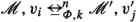
• forth If $wZw'$ and $R_{}wv_{1},\ldots ,v_{n}$ then there are $v_{1}',\ldots ,v_{n}'$ in $W'$ s.t. $R'_{}w'v_{1}',\ldots ,v_{n}'$ and for each $v'_j$ there is a $v_i$ such that $v_i Z v'_j$ where $1\le i,j\le n$.

• back If $wZw'$ and $R'_{}w'v_{1}',\ldots ,v_{n}'$ then there are $v_{1},\ldots ,v_{n}$ in W s.t. $R_{}wv_{1},\ldots ,v_{n}$ and for each $v_i$ there is a $v'_j$ such that $v_i Z v'_j$ where $1\le i,j\le n$.

When Z is a bisimulation linking two states w in ${\mathscr {M}}$ and $w'$ in ${\mathscr {M}}'$ we say that w and $w'$ are $\varPhi$-$wa^n$-bisimilar . When $\varPhi$ is equal to $\mathsf {Prop}$ or is clear from the context, we speak of $wa^n$-bisimulation instead of $\varPhi$-$wa^n$-bisimulation and write instead of . When the models from which w and $w'$ are picked are clear from the context, we also suppress the reference to the models and write for example.

Remark 1

Observe the two subtleties in the above definition: first, the i and j in the forth and back conditions are not necessarily the same, thus we may not have an aligned correspondence of each $v_i$ and $v_i'$; second, in the second part of the forth condition, we require each $v_j'$ to have a corresponding $v_i$, but not the other way around, and similarly in the back condition. This reflects the quantifier alternation in the semantics of $\Box$ in $\textsf {WAML}^n$.

Example 1

Consider the following two 2-models where $\{\langle w,w_1,w_2 \rangle , \langle w,w_2,w_3 \rangle \}$ is the ternary relation in the left model, and $\{\langle v,v_1,v_2 \rangle \}$ is the ternary relation in the right model.

$Z=\{\langle w,v \rangle , \langle w_1, v_1 \rangle , \langle w_2, v_2 \rangle , \langle w_2, v_1 \rangle \}$ is a $wa^2$-bisimulation. And the polyadic modal formula $\lnot \nabla (p, \lnot p)$, not expressible in $\textsf {WAML}^2$, can distinguish w and v.

It is easy to verify that is indeed an equivalence relation. Now we briefly show that $\textsf {WAML}^n$ formulas are invariant under it.

Definition 5

(Modal equivalence) Let ${\mathscr {M}}=(W,R_{},V)$ and ${\mathscr {M}}'=(W',R_{}',V')$ be two n-models, $w \in W$, and $w' \in W'$. Then ${\mathscr {M}}, w\equiv _{\textsf {WAML}^n} {\mathscr {M}}', w'$ iff for all formula $\varphi$ of $\textsf {WAML}^n$, ${\mathscr {M}}, w \models \varphi$ iff ${\mathscr {M}}', w' \models \varphi$. We may also write $w \equiv _{\textsf {WAML}^n} w'$ when it is clear from the context which models w and $w'$ are from.

Proposition 2

Let ${\mathscr {M}}=(W,R_{},V)$ and ${\mathscr {M}}'=(W',R_{}',V')$ be two n-models. Then for every $w\in W$ and $w'\in W'$, if , then $w\equiv _{\textsf {WAML}^n} w'$. In words, $\textsf {WAML}^n$ formulas are invariant under $wa^n$-bisimulation.

Proof

We only consider the modality case. Suppose that and $w\not \models \Box \varphi$. Then there are $v_{1},\ldots ,v_{n}$ s.t. $R_{}wv_{1},\ldots ,v_{n}$, and for each $v_i$, $v_{i}\not \models$ $\varphi$. By the forth condition, there are $v_{1}',\ldots ,v_{n}'$ in $W'$ s.t. $R_{}w'v_{1}',\ldots ,v_{n}'$ and for each $v'_j$ there is a $v_i$ such that $v_i Z v'_j$. From the I.H., for each $v_i$ we have that $v_{i}'\not \models \varphi$. As a result, $w'\not \models \Box \varphi$. For the converse direction (that if $w'\not \models \Box \varphi$ then $w \not \models \Box \varphi$), use the back condition. $\square$

Theorem 1

(Hennessy–Milner Theorem for $\textsf {WAML}^n$) Let ${\mathscr {M}}=(W,R_{},V)$ and ${\mathscr {M}}'=(W',R_{}',V')$ be two image-finite n-models. Then for every $w\in W$ and $w'\in W'$, iff $w\equiv _{\textsf {WAML}^n} w'$.

Proof

As in the standard Kripke semantics, the crucial part is to show that $\equiv _{\textsf {WAML}^n}$ is indeed a $wa^n$-bisimulation between image-finite models. We only verify the forth condition here; the other conditions are easy. Pick w and $w'$ such that ${\mathscr {M}}, w \equiv _{\textsf {WAML}^n} {\mathscr {M}}', w'$ and suppose towards a contradiction that $Rwv_1\dots v_n$ but for each $v_1'\dots v'_n$ such that $R'w'v_1'\dots v'_n$ there is a $v'_j$ such that it is not $\textsf {WAML}^n$-equivalent to any of the $v_i$’s. In image-finite models we can list such $v'_j$ as $u_1, \dots , u_m$. Now for each $u_k$ and each $v_i$ there is a $\varphi _k^i$ that holds on $v_i$ but not on $u_k$. Now consider the formula $\psi =\Diamond (\bigvee _{1\le i\le n}\bigwedge _{1\le k\le m} \varphi _k^i)$. It is not hard to see that $\psi$ holds on w but not $w'$, contradicting that ${\mathscr {M}}, w \equiv _{\textsf {WAML}^n} {\mathscr {M}}', w'$. $\square$

Now we define a notion of k-bisimulation of $\textsf {WAML}^n$ by restricting the maximal depth we care.

Definition 6

($\varPhi$-k-$wa^n$ -bisimulation) Let $\varPhi \subseteq \mathsf {Prop}$. For every n-models ${\mathscr {M}}=(W,R_{},V)$ and ${\mathscr {M}}'=(W',R_{}',V')$ and w and $w'$ from W and $W'$, respectively, we say that ${\mathscr {M}}, w$ and ${\mathscr {M}}', w'$ are $\varPhi$-0-$wa^n$-bisimilar () iff $V(w) \cap \varPhi =V'(w') \cap \varPhi$, and we say that ${\mathscr {M}}, w$ and ${\mathscr {M}}', w'$ are $\varPhi$-$k+1$-$wa^n$-bisimilar () if and the following conditions are satisfied:

• forth If $R_{}wv_{1}\ldots v_{n}$ then there are $v_{1}',\ldots ,v_{n}'$ in $W'$ s.t. $R'_{}v'v_{1}'\ldots v_{n}'$ and for each $v'_j$ there is a $v_i$ such that where $1\le i,j\le n$;

• back If $R'_{}w'v_{1}',\ldots ,v_{n}'$ then there are $v_{1},\ldots ,v_{n}$ in W s.t. $R_{}vv_{1}\ldots v_{n}$ and for each $v_i$ there is a $v'_j$ such that where $1\le i,j\le n$.

We will use $\textsf {WAML}^n_{\varPhi ,k}$-formulas to mean the class of all $\textsf {WAML}^n$ formulas built from $\varPhi$ with modal depth at most k. Again, we suppress the reference to $\varPhi$ when it is just $\mathsf {Prop}$.

By an induction on k one can easily show:

Proposition 3

For any natural number $n \ge 1$, given a finite set $\varPhi$ of propositional letters, the following two hold:

• 1. For all k, up to logical equivalence in ${\mathbb {K}}_n$ there are only finitely many $\textsf {WAML}^n_{\varPhi ,k}$ formulas.

• 2. For all k, every n-model ${\mathscr {M}}$, and every state w in ${\mathscr {M}}$, the set of all $\textsf {WAML}^n_{\varPhi ,k}$ formulas that are satisfied by w is equivalent to a single $\textsf {WAML}^n_{\varPhi , k}$ formula.

Similarly, we can also show the following:

Proposition 4

Suppose $\varPhi$ is a finite set of propositional letters, then given two n-models ${\mathscr {M}}=(W,R_{},V)$ and ${\mathscr {M}}'=(W',R_{}',V')$ the following are equivalent:

• 1. ;

• 2. w and $w'$ agree on all $\textsf {WAML}^n_{\varPhi ,k}$-formulas.

Proof

By an induction on k with a similar strategy in proving Theorem 1. Image-finiteness is not important here because of Proposition 3: while there may be infinitely many successor tuples covering infinitely many worlds when showing the inductive step from k to $k+1$, since there are only finitely many $\textsf {WAML}^n_{\varPhi , k}$ formulas up to logical equivalence in ${\mathbb {K}}_n$, by soundness (which entails that a formula $\varphi$ is true at a world iff all formulas logically equivalent to $\varphi$ are true at that world) and I.H., there are only finitely many -types to consider. $\square$

From the above two propositions, it follows that every -equivalence class can be defined by a single $\textsf {WAML}^n_{\varPhi ,k}$-formula.

We can translate each $\textsf {WAML}^n$ formula to an equivalent $\textsf {FOL}$ formula with one free variable and $n+1$-ary relation symbols in a meaning preserving way.

Definition 7

(Standard translation) Define by simultaneous recursion the following family $\{ST_x\}$ of functions from $\textsf {WAML}^n$ to $\textsf {FOL}$ (with countably many unary predicates corresponding to the elements in $\mathsf {Prop}$ and an $n+1$-ary relation symbol R) indexed by the variables in $\textsf {FOL}$:

$$\begin{aligned} ST_x(p)&=Px; \\ ST_x(\lnot \varphi )&= \lnot ST_x(\varphi ); \\ ST_x(\varphi \wedge \psi )&= ST_x(\varphi )\wedge ST_x(\psi ); \\ ST_x(\Box \varphi )&= \forall y_1\forall y_2\dots \forall y_n (R xy_1y_2\dots y_n\rightarrow ST_{y_1}(\varphi )\vee \dots \vee ST_{y_n}(\varphi )). \end{aligned}$$

Following a similar strategy as in Otto (2004), we will show a van Benthem–Rosen characterization theorem for $\textsf {WAML}^n$: a $\textsf {FOL}$ formula is equivalent to the translation of a $\textsf {WAML}^n$ formula (over finite n-models) if and only if it is invariant under $wa^n$-bisimulations (over finite n-models).

First we need to define a notion of unraveling with respect to n-ary models similarly to models with binary relations. We use an example of a graph with ternary relations to illustrate the intuitive idea behind the general n-ary unraveling, which is first introduced in de Rijke (1993).

Example 2

Consider the 2-model $\langle \{w,v,u,t\},$ $\{\langle w, u,t \rangle ,$ $\langle u,t,u \rangle ,$ $\langle t,w,v \rangle \}, V \rangle$. It is quite intuitive to first unravel it into a tree with pairs of states as nodes, illustrated below:

To turn it into a 2-model, we need to define the new ternary relations. For each triple $\langle s_0,s_1,s_2 \rangle$ of pairs, $\langle s_0, s_1, s_2 \rangle$ is in the new ternary relation iff $s_1$ and $s_2$ are successors of $s_0$ in the above graph and the triple of underlined worlds in $s_0, s_1, s_2$ respectively is in the original ternary relation. For example, $\langle \langle u,{\underline{t}} \rangle ,\langle {\underline{w}},v \rangle ,\langle w,{\underline{v}} \rangle \rangle$ is in the new ternary relation since $\langle t,w,v \rangle$ is in the original ternary relation.

In general, we can use the n-tuples of the states in the original model together with a natural number $k\in [1,n]$ as the basic building blocks for the unraveling of an n-model. For example, $\langle w, v, u, 2 \rangle$ means the second state is the underlined one. To make the definition uniform, we define the root of an unraveling from w as the sequence $\langle w,\dots ,w,1 \rangle .$ Like the unraveling for a binary graph, formally we will use sequences of such building blocks as the nodes in the unraveling of an n-model. For example, the left-most node $\langle {\underline{t}},u \rangle$ in the above example will be coded by $\langle \langle w,w,1 \rangle ,\langle u,t,1 \rangle ,\langle t, u ,1 \rangle \rangle$. This leads to the following definition.

Definition 8

Given an n-model ${\mathscr {M}}=\langle W,R,V\rangle$ and $w\in W$, we first define the binary (in the sense that the relation in the unraveling is binary) unraveling ${\mathscr {M}}^b_{w}$ of ${\mathscr {M}}$ around w as $\langle W_w, R^b, V' \rangle$ where:

• $W_w$ is the set of sequences $\langle \langle \vec {v}_0,i_0\rangle ,\langle \vec {v}_{1},i_{1}\rangle ,\ldots ,\langle \vec {v}_{m},i_{m}\rangle \rangle$ where:

  • $m\in {\mathbb {N}}$;

  • for each $j\in [0,m]$, $\vec {v}_{j}\in W^n$ and $i_{j}\in [1, n]$ such that $R(\vec {v}_{j}[i_{j}])\vec {v}_{j+1}$;⁹

  • $\vec {v}_0$ is the constant n-sequence $\langle w,\dots ,w\rangle$ and $i_0=1$;

• as convenient and also conceptually important notations, for each $s \in W_w$ with its last item being $\langle \vec {v}, i \rangle$, define $e(s) = \vec {v}$, $o(s) = i$, and $r(s) = \vec {v}[i]$; intuitively, s records a history of traveling in ${\mathscr {M}}$ starting from w where in each step we choose an edge emanating from the current world and an arrow in the edge (since an edge can be seen as a tuple of n arrows) and then follow that arrow to the next world; thus, we understand e(s) as the last edge used in the traveling history, o(s) as the index of the arrow in the last edge used, and r(s) as the “current” world in history s;

• $R^bss'$ iff $s'$ extends s with some $\langle \vec {v}, i \rangle$;

• $V'(s)=V(r(s))$.

The unraveling ${\mathscr {M}}_w$ then is defined as $\langle W_w, R', V' \rangle$ where $R'$ is the $n+1$-ary relation on $W_w$ satisfying the condition that $R's_0 s_1\dots s_n$ iff there is an n-tuple $\vec {v} = \langle v_1, v_2, \ldots , v_n\rangle$ of W such that $Rr(s_0)v_1v_2\ldots v_n$ and that $s_i$ is precisely $s_0$ extended with $\langle \vec {v}, i \rangle$ for all $i = 1 \ldots n$. In other words, $R's_0 s_1\dots s_n$ iff for each i from 1 to n, $R's_0s_i$, $e(s_i) = e(s_1)$, $o(s_i) = i$, and $Rr(s_0)r(s_1)\cdots r(s_n)$ (this condition in fact follows from the previous three given the definition of $W_w$).

Finally, let the bounded unraveling ${\mathscr {M}}_w|_l$ be the submodel of ${\mathscr {M}}_w$ obtained by restricting the domain of ${\mathscr {M}}_w$ to sequences of length at most l.

Remark 2

The unraveling ${\mathscr {M}}_w$ is clearly tree-like since ${\mathscr {M}}_w^b$ is clearly tree-like and $R'$ is obtained by grouping, for each $s \in W_w$, the edges in $R^b$ from s to the children of s according to the first n coordinate of these children.

Note that, intuitively, the r defined above reveals for each sequence $s \in {\mathscr {M}}_w$ the state in the original model ${\mathscr {M}}$ this sequence s corresponds to. Then, it is not hard to show the following.

Proposition 5

The above r (viewed as a relation) is a $wa^n$-bisimulation between ${\mathscr {M}}_{w}$ and ${\mathscr {M}}$. In fact, r is a p-morphism (over n-models) from ${\mathscr {M}}_w$ to ${\mathscr {M}}$.

Proof

• Invariance: by definition of $V'$.

• Forth condition: If $R'xy_{1}\ldots y_{n}$, then by the definition of $R'$, $Rr(x)r(y_{1})\ldots r(y_{n})$.

• Back condition: If $Rr(x)z_{1}\ldots z_{n}$, then let $y_{i}$ be the extension of x by $\langle \langle z_{1},\ldots ,z_{n}\rangle ,i \rangle$, for each i from 1 to n. By our definition of $W_{w}$, $y_{i}\in W_{w}$ and $r(y_{i})=z_{i}$, which shows that $R'xy_{1}\ldots y_{n}$. $\square$

Now we have all the ingredients to prove the following characterization theorem. Note that the characterization works with or without the finite model constraints.

Theorem 2

A first-order formula $\alpha (x)$ is invariant under (over finite models) iff $\alpha (x)$ is equivalent to a $\textsf {WAML}^n$ formula (over finite models).

We will prove this theorem through the general strategy in Otto (2004). First, we show the following finitary version of the characterization theorem.

Theorem 3

A first-order formula $\alpha (x)$ is invariant under (on finite models) iff $\alpha (x)$ is equivalent to a $\textsf {WAML}^n_k$ formula (on finite models).

Proof

The right-to-left direction is trivial. For the left-to-right direction, let $\varPhi$ be the set of propositional letters in $\mathsf {Prop}$ whose corresponding unary predicate occurs in $\alpha (x)$. Then $\varPhi$ is finite, and by the principle of irrelevance in first-order logic (changing the valuation of propositional letters not in $\varPhi$ does not affect the truth value of $\alpha (x)$), $\alpha (x)$ now must be invariant under (if , then by making every propositional letters not in $\varPhi$ false everywhere in ${\mathscr {M}}$ and ${\mathscr {M}}'$ and obtaining ${\mathscr {N}}, w$ and ${\mathscr {N}}', w'$ respectively, ). Then, by Propositions 3 and 4, has only finitely many equivalence classes (either on the class of all models or the class of finite models), each defined by a formula in $\textsf {WAML}^n_{\varPhi , k}$. Given that $\alpha (x)$ is invariant under , its model class is a finite union of those equivalence classes, and thus it is equivalent to a formula in $\textsf {WAML}^n_k$, namely the disjunction of the formulas defining those equivalence classes. $\square$

Clearly, the gap from Theorem 3 to 2 is filled by the following lemma:

Lemma 1

A first-order formula $\alpha (x)$ is invariant under (over finite models) iff $\alpha (x)$ is invariant under for some l (over finite models).

Again, the right-to-left direction is trivial. To prove the left-to-right direction, we take the following detour strategy. We need to find the right l such that the truth value of $\alpha$ is preserved by moving to a partial unraveling ${\mathscr {M}}_w|_l$ of the model where the maximal length of each point (recall that it is a sequence) is bounded by l.

So the following lemma, which is the most non-trivial part, is sufficient for our goal.

Lemma 2

(Locality) If an $\mathsf {FOL}$ formula $\alpha (x)$ is invariant under (over finite models), then there is $l \in {\mathbb {N}}$, for any n-model ${\mathscr {M}}, w$, ${\mathscr {M}}\Vdash \alpha (x)[w]$ iff ${\mathscr {M}}_w|_{l}\Vdash \alpha (x)[\langle \langle \vec {w},1 \rangle \rangle ]$. In fact, if the quantifier rank of $\alpha$ is q, we can pick $l = 2^q$.

Proof

Let q be the quantifier rank of $\alpha (x)$, and let $l=2^q$. Then let the partial unraveling ${\mathscr {M}}^+_w|_l$ of ${\mathscr {M}}$ be the model coming from ${\mathscr {M}}_w|_{l+1}$ where each leaf node s is replaced by a copy of the original ${\mathscr {M}}, r(s)$ (recall that r is defined in Definition 8). The reason we use ${\mathscr {M}}_w|_{l+1}$, the unraveling of ${\mathscr {M}}, w$ restricted to level $l+1$, for the partial unraveling ${\mathscr {M}}^+_w|_l$ to level l is to keep the attached copies of ${\mathscr {M}}$ away from the leaves of ${\mathscr {M}}_w|_l$. Now we construct two pointed models ${\mathscr {M}}^*, w^*$ and ${\mathscr {N}}^*, v^*$:

• let ${\mathscr {M}}^*$ be the disjoint union of q isomorphic copies of ${\mathscr {M}}_w|_l$ and another $q+1$ isomorphic copies of partial unraveling ${\mathscr {M}}^+_w|_l$, and let $w^*$ be the root of one of those ${\mathscr {M}}^+_w|_l$;

• let ${\mathscr {N}}^*$ be the disjoint union of q isomorphic copies of ${\mathscr {M}}^+_w|_l$ and $q+1$ isomorphic copies of ${\mathscr {M}}_w|_l$, and let $v^*$ be the root of one of those ${\mathscr {M}}_w|_l$.

Set theoretically, the copies of ${\mathscr {M}}_w|_l$ and ${\mathscr {M}}^+_w|_l$ are constructed by taking the product of them with $\{1, 2, \ldots , q+1\}$. It is clear that . Moreover, based on Proposition 5, we can show that by extending r. Hence, we will be done if we can show that ${\mathscr {M}}^*, w^* \equiv _{\mathsf {FOL}_q} {\mathscr {N}}^*, v^*$. Intuitively, ${\mathscr {M}}^*,w^*$ and ${\mathscr {N}}^*,v^*$ are “forests” pictured as follows (q and $q+1$ denote the number of copies):

Given the special composition of the two models, for each w in ${\mathscr {M}}^*$ or ${\mathscr {N}}^*$, let c(x) be the point in ${\mathscr {M}}_w^+|_l$ that x corresponds to. More precisely, since we build the copies of ${\mathscr {M}}_w^+|_l$ and ${\mathscr {M}}_w|_l$ by taking the products of them with $\{1, 2, \ldots , q, q+1\}$, c(x) is just the first coordinate of x. Note that if x is in a copy of ${\mathscr {M}}_w|_l$, c(x) is also in ${\mathscr {M}}_w^+|_l$ since ${\mathscr {M}}_w|_l$ is in fact a submodel of ${\mathscr {M}}_w^+|_l$. To conveniently see whether x in ${\mathscr {M}}^*$ or ${\mathscr {N}}^*$ corresponds to the difference between ${\mathscr {M}}_w^+|_l$ and ${\mathscr {M}}_w|_l$ or not, let $t(x) = 0$ if c(x) is in ${\mathscr {M}}_w|_l$ and $t(x) = 1$ otherwise.

Now our goal is to show that ${\mathscr {M}}^*,w^* \equiv _{\textsf {FOL}_q} {\mathscr {N}}^*,v^*$. For this, for each $u, v \in {\mathscr {M}}^*$ (resp. ${\mathscr {N}}^*$), let d(u, v) be the distance between u and v, i.e., the length of the shortest path between u and v, in the (undirected) Gaifman graph of ${\mathscr {M}}^*$ (resp. ${\mathscr {N}}^*$). Recall that given ${\mathscr {M}}^* = \langle W_{{\mathscr {M}}^*}, R_{{\mathscr {M}}^*}\rangle$, the Gaifman graph $G({\mathscr {M}}^*)$ of ${\mathscr {M}}^*$ is $\langle W_{{\mathscr {M}}^*}, R \rangle$ where $\langle x, y \rangle \in R$ iff $x \not = y$ and $\vec {v} \in R_{{\mathscr {M}}^*}$ for some $\vec {v}$ including both x and y. The same definition goes for ${\mathscr {N}}^*$.¹⁰ Furthermore, for any finite sequence $\vec {u}$ of elements in ${\mathscr {M}}^*$ (resp. ${\mathscr {N}}^*$) and any natural number k, let $U_k(\vec {u})$ be the restriction of ${\mathscr {M}}^*$ (resp. ${\mathscr {N}}^*$) to the set of elements whose distances to one of the elements in $\vec {u}$ are no greater than k.

Then, consider the family $I = \langle I_m \rangle _{m = 0, \ldots , q}$ of sets of partial functions from ${\mathscr {M}}^*$ to ${\mathscr {N}}^*$ where each $I_m$ consists of partial functions f from ${\mathscr {M}}^*$ to ${\mathscr {N}}^*$ satisfying the following conditions:

• f is injective, and $|{\textit{dom}}(f)| = m+1$;

• for any $x \in {\textit{dom}}(f)$, $c(x) = c(f(x))$; moreover, there exists $y \in U_{2^{q-m}}(x)$ such that $t(y) = 1$ iff there exists $y' \in U_{2^{q-m}}(f(x))$ such that $t(y') = 1$; note that the two conditions here force $U_{2^{q-m}}(x)$ to be isomorphic to $U_{2^{q-m}}(f(x))$ by matching points from the two submodels that correspond to the same point; in other words, they are isomorphic by c to the same submodel of ${\mathscr {M}}^+|_l$;

• for any $x, y \in {\textit{dom}}(f)$, $d(x, y) \le 2^{q-m}$ iff $d(f(x), f(y)) \le 2^{q-m}$.¹¹

Clearly then, the function $f = \{\langle w^*, v^*\rangle \}$ is in $I_0$. Furthermore, for every $m \in \{0, \ldots , q\}$, every $f \in I_m$ is a partial isomorphism for the following reason: if $\vec {v} = \langle v_1, \ldots , v_n \rangle$ consisting of points in ${\textit{dom}}(f)$ is in the relation of ${\mathscr {M}}^*$, then by the definition of the Gaifman graph and the distance function d, $d(v_1, v_i) \le 1 \le 2^{q-m}$. Hence, by the third condition of the definition of I, $d(f(v_1), f(v_i)) \le 2^{q-m}$ as well. This means that all $v_i$’s are in $U_{2^{q-m}}(v_1)$ and all $f(v_i)$’s are in $U_{2^{q-m}}(f(v_1))$. Then, since $U_{2^{q-m}}(v_1)$ is isomorphic to $U_{2^{q-m}}(f(v_1))$ by matching points corresponding to the same point using c, and since $v_i$ and $f(v_i)$ do correspond to the same point, $\langle f(v_1), \ldots , f(v_n) \rangle$ is in the relation of ${\mathscr {N}}^*$.

Hence, to conclude that ${\mathscr {M}}^*, w^* \equiv _{\mathsf {FOL}_q} {\mathscr {N}}^*, v^*$, we only need to show that I has the back and forth condition required for $I: {\mathscr {M}}^* \cong _q {\mathscr {N}}^*$. Pick an arbitrary f in $I_m$ and any $x \in {\mathscr {M}}^*$ not already in ${\textit{dom}}(f)$. Then, to extend f to g by adding x to its domain, there are two cases.

• If there is $y \in {\textit{dom}}(f)$ such that $d(x, y) \le 2^{q-m-1}$, let $x'$ be the element in ${\mathscr {N}}^*$ such that $c(x') = c(x)$ and $d(x', f(y)) < \infty$ ($x'$ and f(y) are in the same copy). This $x'$ is well-defined (its choice does not depend on the choice of y) since f preserves distances no greater than $2^{q-m-1}$ and the distance function satisfies the triangle inequality. Then let $g = f \cup \{\langle x, x'\rangle \}$. To show that $g \in I_{m+1}$, we need to show the three conditions in the definition of I. The first and the third are easy. For the second, the only interesting case is for the newly added $x \in {\textit{dom}}(g) {\setminus } {\textit{dom}}(f)$. In this case, it is enough to notice that, picking a $y \in {\textit{dom}}(f)$ such that $d(x, y) \le 2^{q-m-1}$, $U_{2^{q-(m+1)}}(x) \subseteq U_{2^{q-m}}(y)$ and also $U_{2^{q-(m+1)}}(x') \subseteq U_{2^{q-m}}(f(y))$.

• If there is no $y \in {\textit{dom}}(f)$ such that $d(x, y) \le 2^{q-m-1}$, let $x'$ be an element in ${\mathscr {N}}^*$ such that (1) $c(x') = c(x)$, (2) $d(x', f(y)) = \infty$ for all $y \in {\textit{range}}(f)$ (namely that $x'$ is not on any copy containing elements in ${\textit{range}}(f)$), and (3) there exists $y \in U_{2^{q-m}}(x)$ such that $t(y) = 1$ iff there exists $y' \in U_{2^{q-m}}(x')$ such that $t(y') = 1$. Since we have at least q many copies of both ${\mathscr {M}}_w^+|_l$ and ${\mathscr {M}}_w|_l$, such an $x'$ can always be found. Letting $g = f \cup \{\langle x, x'\rangle \}$, clearly $g \in I_{m+1}$.

The back condition where we start with picking an $x \in {\mathscr {N}}^*$ is completely symmetric. Hence, we are done showing that ${\mathscr {M}}^*, w^* \equiv _{\mathsf {FOL}_q} {\mathscr {N}}^*, v^*$ and also the whole lemma.$\square$

4 Interpolation

By a standard strategy in Hansen et al. (2009), we know that the basic polyadic modal logics ($\textsf {PML}$) have the Craig Interpolation Property (CIP). Moreover, in Santocanale et al. (2010), the authors proved that the minimal monotonic modal logic M has uniform interpolation. Furthermore, we know that the basic modal logic ${\mathbb {K}}$ also has Uniform Interpolation from Andréka et al. (1995) and Andréka et al. (1998). From the following three aspects then, one may conjecture that the basic $\textsf {WAML}$ systems ${\mathbb {K}}_{n}$ should have interpolation too:

• 1. $\textsf {WAML}$ can be treated as a fragment of $\textsf {PML}$.

• 2. ${\mathbb {K}}_{n}$ is regarded as a general version of ${\mathbb {K}}$, since ${\mathbb {K}}$ is just ${\mathbb {K}}_{1}$.

• 3. ${\mathbb {K}}_{n}$ can be viewed as a special kind of monotonic modal logics.

As further evidence of how enticing this conjecture is, it is claimed in Pattinson (2013) that every rank-1 monotone modal logic¹² with finitely many modalities has uniform interpolation (a property stronger than CIP), and the logics ${\mathbb {K}}_n$ for $n \ge 2$ are paradigmatic rank-1 monotone modal logics.

However, none of the ${\mathbb {K}}_{n}$’s for $n \ge 2$ has CIP, and the claim in Pattinson (2013) is retracted in Seifan et al. (2017), though using a different counterexample. In fact, the counterexamples to the CIP of ${\mathbb {K}}_n$’s are surprisingly simple and illuminating. Among them, the counterexamples to ${\mathbb {K}}_n$’s with $n \ge 3$ are easier, where we do not even need more than 1 successor tuple for any point. The counterexample to ${\mathbb {K}}_2$, however, requires more than 1 successor tuple: we will show that if we only consider 2-models where each state has no more than 1 successor tuple, their logic does have CIP.

Before we state the counterexamples, let us first clarify what do we mean by “a counterexample” to CIP for ${\mathbb {K}}_n$.

Lemma 3

Let n be a non-zero natural number. If there are two pointed n-models ${\mathscr {M}}, w$ and ${\mathscr {N}}, v$ and two formulas $\varphi$ and $\psi$ such that

• 1. ${\mathscr {M}}, w\models \varphi$ and ${\mathscr {N}}, v\models \psi$;

• 2. ${\mathbb {K}}_n \vdash \varphi \rightarrow \lnot \psi$;

• 3. letting $\varPhi$ be the set of all the propositional letters that appear both in $\varphi$ and $\psi$, for any formula $\gamma$ in $\textsf {WAML}$ such that only letters in $\varPhi$ appear, ${\mathscr {M}}, w \models \gamma$ iff ${\mathscr {N}}, v \models \gamma$;

then ${\mathbb {K}}_n$ does not have the Craig Interpolation Property.

Proof

Assume for contradiction that ${\mathbb {K}}_n$ has CIP. Then since ${\mathbb {K}}_n \vdash \varphi \rightarrow \lnot \psi$, there is an interpolant $\gamma$ such that:

• ${\mathbb {K}}_n \vdash \varphi \rightarrow \gamma$ and ${\mathbb {K}}_n \vdash \gamma \rightarrow \lnot \psi$;

• only letters in $\varPhi$ appear in $\gamma$.

Since ${\mathscr {M}}, w \models \varphi$ with ${\mathscr {M}}$ being an n-model and ${\mathbb {K}}_n \vdash \varphi \rightarrow \gamma$, by soundness, ${\mathscr {M}}, w \models \gamma$. Then ${\mathscr {N}}, v \models \gamma$ by 3. Then using ${\mathbb {K}}_n \vdash \gamma \rightarrow \lnot \psi$ and soundness again, ${\mathscr {N}}, v \models \lnot \psi$. This contradicts that ${\mathscr {N}}, v \models \psi$. $\square$

Given this proposition, a pair of pointed n-models and a pair of formulas satisfying the antecedent constitute a counterexample to CIP. Now we proceed to provide them for each ${\mathbb {K}}_n$ with $n \ge 2$.

Example 3

Consider the following two 2-models where $\{\langle w,w_1,w_1 \rangle ,\langle w,w_2,w_3 \rangle \}$ is the ternary relation in the left model ${\mathscr {M}}_2$, and $\{\langle v,v_1,v_2 \rangle \}$ is the ternary relation in the right model ${\mathscr {N}}_2$, where the valuations are as in the diagram.

Then set $\varphi _2 = \Box (\lnot p \vee \lnot q) \wedge \Diamond q$ and $\psi _2 = \Box (p \wedge r) \wedge \Box (p \wedge \lnot r)$. It is easy to see that ${\mathscr {M}}_2, w \models \varphi _2$ and ${\mathscr {N}}_2, v \models \psi _2$. To see that ${\mathbb {K}}_2\vdash \varphi _2 \rightarrow \lnot \psi _2$, consider the following derivation, where to make long Boolean combinations readable, we write negation of propositional letters as overline, omit $\wedge$ between purely Boolean formulas and replace $\vee$ with |.

• $\vdash _2 \Box (\bar{p} | \bar{q}) \wedge \Box rp \wedge \Box \bar{r}p \rightarrow \Box (((\bar{p} | \bar{q})rp) | ((\bar{p} | \bar{q})\bar{r}p)| rp\bar{r}p)$ $\mathtt {K}_2$

• $\vdash _2 (((\bar{p} | \bar{q})rp) | ((\bar{p} | \bar{q})\bar{r}p)| rp\bar{r}p) \rightarrow p{\bar{q}}$ A propositional tautology

• $\vdash _2 \Box (\bar{p} | \bar{q}) \wedge \Box rp \wedge \Box \bar{r}p \rightarrow \Box p\bar{q}$ PL,RM

• $\vdash _2 \varphi _2 \wedge \psi _2 \rightarrow \Box p\bar{q} \wedge \Diamond q$ PL

• $\vdash _2 \varphi _2 \wedge \psi _2 \rightarrow \Box \bar{q} \wedge \lnot \Box \bar{q}$ PL, $\mathtt {RM}$

• $\vdash _2 \varphi _2 \rightarrow \lnot \psi _2$ PL

Here PL means propositional reasoning. Hence, we are done with the first two requirements for this pair of models and formulas to count as a counterexample. For the last requirement, note that

$$\begin{aligned} Z=\{\langle w,v \rangle , \langle w_1, v_1 \rangle , \langle w_1, v_2 \rangle , \langle w_2, v_1 \rangle ,\langle w_2, v_2 \rangle \} \end{aligned}$$

is a $\varPhi$-$wa^2$-bisimulation for $\varPhi = \{p\}$. Hence, by Proposition 2, for any formula $\gamma$ with p the only propositional letter, ${\mathscr {M}}_2, w \models \gamma$ iff ${\mathscr {N}}_2, v \models \gamma$. But p is the only common propositional letters in $\varphi _2$ and $\psi _2$. So, ${\mathscr {M}}, w$, ${\mathscr {N}}, v$, $\varphi _2$, and $\psi _2$ form a counterexample to CIP for ${\mathbb {K}}_2$.

Example 4

Consider the following two 3-models where $\{\langle w,w_1,w_2,w_3 \rangle \}$ is the relation in ${\mathscr {M}}_3$ and $\{\langle v,v_1,v_2,v_3 \rangle \}$ is the relation in ${\mathscr {N}}_3$.

Then set $\varphi _3= \Box p\bar{q} \wedge \Box pq \wedge \Diamond (p|\bar{p})$, $\psi _3= \Box \bar{p}r \wedge \Box \bar{p}\bar{r} \wedge \Diamond (p|\bar{p})$. Clearly ${\mathscr {M}}_3, w \models \varphi _3$ and ${\mathscr {N}}_3, v \models \psi _3$. Further, ${\mathbb {K}}_2 \vdash \varphi _3 \rightarrow \lnot \psi _3$ since we have the following derivation.

• $\vdash _3 \Box p\bar{q} \wedge \Box pq \wedge \Box \bar{p}r \wedge \Box \bar{p}\bar{r} \rightarrow \Box (p\bar{q}pq | p\bar{q}\bar{p}r | p \bar{q}\bar{p}\bar{r} | pq\bar{p}r | pq\bar{p}\bar{r} | \bar{p}r\bar{p}\bar{r} )$ $\mathtt {K}_3$

• $\vdash _3 \Box p\bar{q} \wedge \Box pq \wedge \Box \bar{p}r \wedge \Box \bar{p}\bar{r} \rightarrow \Box p\bar{p}$ PL,

• $\vdash _3 \varphi _3 \wedge \psi _3 \rightarrow \Box p\bar{p} \wedge \Diamond (p|\bar{p})$ PL, $\mathtt {RM}$

• $\vdash _3 \varphi _3 \rightarrow \lnot \psi _3$ PL

Finally, note that $Z=\{\langle w,v \rangle , \langle w_1, v_3 \rangle , \langle w_2, v_3 \rangle , \langle w_3, v_1 \rangle ,\langle w_3, v_2 \rangle \}$ is a $\{p\}$-$wa^3$-bisimulation.

The above example can be naturally generalized for each ${\mathbb {K}}_n$ with $n > 3$. Let m be the least natural number s.t. $2^{m} \ge n-1$ and pick m many distinct propositional letters $r_1, \ldots , r_m$ from $\mathsf {Prop}$ that are different from p and q. Then for each i from 1 to $n-1$, we can associate a distinct conjunction $\rho _i$ of literals formed from $r_j$’s so that $\rho _i \wedge \rho _{i'}$ are incompatible for each $i \not = i'$. Then we can state the general counterexample.

Example 5

Consider the following two n-models where $\{\langle w,w_1,\ldots ,w_n \rangle \}$ is the relation in ${\mathscr {M}}_n$, and $\{\langle v,v_1,\ldots ,v_n \rangle \}$ is the relation in ${\mathscr {N}}_n$.

Set $\varphi _n = \Box (p \wedge \lnot q) \wedge \Box (p \wedge q) \wedge \Diamond \top$ and $\psi _n = \bigwedge _{i = 1}^{n-1}\Box (\lnot p \wedge \rho _{i}) \wedge \Diamond \top$. Clearly ${\mathscr {M}}_n, w \models \varphi _n$ and ${\mathscr {N}}_n, v \models \psi _n$. It is also easy to see that by $\mathtt {K}_n$, we can derive $(\Box (p \wedge \lnot q) \wedge \Box (p \wedge q) \wedge \bigwedge _{i = 1}^{n-1}\Box (\lnot p \wedge \rho _i)) \rightarrow \Box \bot$. With this we can then easily derive $\varphi _n \rightarrow \lnot \psi _n$ in ${\mathbb {K}}_n$. Finally, note that p is the only common propositional letter in $\varphi _n$ and $\psi _n$ and that $Z=\{\langle w,v \rangle , \langle w_1, v_1 \rangle , \langle w_2, v_1 \rangle \} \cup \{w_3,\ldots ,w_n\} \times \{v_2,\ldots ,v_n\}$ is a $\{p\}$-$wa^n$-bisimulation.

With the examples and Lemma 3, the main theorem of this section follows.

Theorem 4

For any $n \ge 2$, ${\mathbb {K}}_n$ does not have the Craig Interpolation Property.

A natural question follows immediately: can we find logics extending ${\mathbb {K}}_n$’s that have CIP? To be more precise, we define n-normal modal logics:

Definition 9

An n-normal modal logic ${\mathsf {L}}$ (with $n \ge 1$ a natural number) is a subset of the language of $\textsf {WAML}$ that contains all propositional tautologies and the axiom $\mathtt {K}_n$, and is closed under modus ponens, uniform substitution, the rule $\mathtt {RM}$, and the necessitation rule $\mathtt {N}$.

According to Definition 3, ${\mathbb {K}}_n$ is the smallest n-normal modal logic. For any formula $\varphi$ (resp. set of formulas X) in the language of $\textsf {WAML}$, we write ${\mathbb {K}}_n\varphi$ (resp. ${\mathbb {K}}_n X$) for the smallest n-normal modal logic containing $\varphi$ (resp. all formulas in X).

Now, note that Lemma 3 uses only the soundness of the logics: we can replace ${\mathbb {K}}_n$ there with any logic that is valid on the underlying frames of the “counterexamples”. Thus, just by using the same counterexamples above, we have the following corollary:

Corollary 1

If L is an n-normal modal logic and is valid on the underlying frames of both ${\mathscr {M}}_n$ and ${\mathscr {N}}_n$, then L does not have CIP. For example, ${\mathbb {K}}_n(\Box p \rightarrow \Box \Box p)$ does not have CIP, since the underlying frames of ${\mathscr {M}}_n$ and ${\mathscr {N}}_n$ validate $\Box p \rightarrow \Box \Box p$ trivially.

Thus, to restore CIP, we need formulas that rule out the counterexamples. Note that in the counterexample to the CIP of ${\mathbb {K}}_2$ we gave above, we used two distinct successor tuples. Recall that in the standard Kripke semantics, the formula $\Box (p \vee q) \rightarrow (\Box p \vee \Box q)$, which we now refer to by ${\mathtt {C}}^{*}$, defines the property of having no more than one successor (the property of being partially functional). Relative to 2-frames, ${\mathtt {C}}^{*}$ does not define partial functionality. But we will show that it is very close, and at the very least, it rules out the counterexample above for ${\mathbb {K}}_2$: ${\mathtt {C}}^{*}$ is not valid on ${\mathscr {M}}_2$ since it is false at w once we change the valuation of p so that p is also false at $w_2$. For the rest of this section, we show that the addition of ${\mathtt {C}}^{*}$ to ${\mathbb {K}}_2$ restores CIP. For ${\mathbb {K}}_n$ with $n > 2$, however, ${\mathtt {C}}^{*}$ will not restore CIP, since the counterexamples above for them still works.

The first step toward the CIP of ${\mathbb {K}}_2{\mathtt {C}}^{*}$ is to provide the first-order correspondent ${\mathtt {C}}^{*}$ relative to n-frames. Intuitively, it says that if a point w has an n-tuple successor, then w has a minimal n-tuple successor.

Proposition 6

An n-frame ${\mathscr {F}}=\langle W, R\rangle$ validates ${\mathtt {C}}^{*}$ if and only if for each $w \in W$:

$$\begin{aligned} \begin{aligned}&\exists \langle x_1,\ldots ,x_n \rangle (wRx_1\ldots x_n) \\&\quad \rightarrow \exists \langle a_1,\ldots ,a_n \rangle (wRa_1\ldots a_n \wedge \forall \langle b_1,\ldots ,b_n \rangle (wRb_1\ldots b_n \rightarrow \{a_1,\ldots ,a_n\}\\&\quad \subseteq \{b_1,\ldots ,b_n\})). \end{aligned}\nonumber \\ \end{aligned}$$

(1)

Proof

Let ${\mathscr {F}}=\langle W, R\rangle$ be an n-frame. It is easy to observe that ${\mathscr {F}}$ validates ${\mathtt {C}}^{*}$ iff ${\mathscr {F}}$ validates $(\Diamond p \wedge \Diamond q) \rightarrow \Diamond (p \wedge q)$, so we focus on $(\Diamond p \wedge \Diamond q) \rightarrow \Diamond (p \wedge q)$ instead.

The right to left direction is as usual easy to check: the witness for the truth of $\Diamond (p \wedge q)$ is always the tuple $\langle a_1, \ldots , a_n\rangle$ claimed to exist in the consequent of (1). For the other direction, suppose ${\mathscr {F}}$ validates $(\Diamond p \wedge \Diamond q) \rightarrow \Diamond (p \wedge q)$. To facilitate the proof, we introduce the following notations: let $U(s) = \{a_1, a_2, \ldots , a_n\}$ for any n-tuple $s = \langle a_1, a_2, \ldots , a_n\rangle$, and let $U(X) = \{U(s) \mid s \in X\}$ for any set X of n-tuples. Also, let $R(w) = \{\langle w_1, w_2, \ldots , w_n \rangle \in W^n \mid Rww_1w_2\ldots w_n\}$, the set of successor n-tuples of w in R. Now pick any $w \in W$. Using the notations above, our goal is to show that if R(w) is non-empty, then there is an $s \in R(w)$ such that for all $s' \in R(w)$, $U(s) \subseteq U(s')$. So suppose that R(w) is non-empty. To find the required s, we only need to show that there is $Z \in U(R(w))$ that is a subset of every element in U(R(w)) since if so, we can then let s by any $s_0 \in R(w)$ such that $U(s_0) = Z$. To do this, we first show that U(R(w)) is a directed family of sets: for any $X,Y \in U(R(w))$, there is some $Z \in U(R(w))$ such that $Z \subseteq X \cap Y$. Pick any $X, Y \in U(R(w))$ and $s, t \in R(w)$ such that $X = U(s)$ and $Y = U(t)$. Let V be any valuation on ${\mathscr {F}}$ such that $V(p)=X, V(q)=Y$, and let ${\mathscr {M}}=\langle {\mathscr {F}},V \rangle$. Then, ${\mathscr {M}}, w \models \Diamond p \wedge \Diamond q$. Since ${\mathscr {F}}\models (\Diamond p \wedge \Diamond q) \rightarrow \Diamond (p \wedge q)$, ${\mathscr {M}},w \models \Diamond (p \wedge q)$. So there must be $u \in R(w)$ (which means that $U(u) \in U(R(w))$) such that ${\mathscr {M}}, x \models p \wedge q$ for each $x \in U(u)$. Since $V(p) = X$ and $V(q) = Y$, $U(u) \subseteq X \cap Y$. This shows that U(R(w)) is directed. By a simple induction, for any finite $\varDelta \subseteq U(R(w))$, there is $Z \in U(R(w))$ such that $Z \subseteq \bigcap \varDelta$. Now notice that R(w) is a set of n-tuples, so every set in U(R(w)) has at most n elements. Pick any $X \in U(R(w))$ and let $\varDelta = \{Z \in U(R(w)) \mid Z \subseteq X\}$. By directedness, for every $Y \in U(R(w))$, there is $Z \in \varDelta$ such that $Z \subseteq Y$. Moreover, $\varDelta$ is finite ($|\varDelta | \le 2^n$). So pick $Z \in U(R(w))$ such that $Z \subseteq \bigcap \varDelta$. Then Z is a subset of every element in $\varDelta$, and by transitivity, a subset of every element in U(R(w)). This concludes the proof. $\square$

The above property may seem convoluted at first sight, but once we allow for the flexibility of taking bisimilar models, essentially we are looking at the standard property of being partially functional on standard Kripke frames. To show this, we introduce the concept of core. Since our focus is on ${\mathbb {K}}_2{\mathtt {C}}^{*}$ with the semantics based on 2-models, we state the definitions only for 2-models. The generalization to n-models is straightforward.

Definition 10

For any $X \subseteq W^2$ and $\langle a_1, a_2\rangle \in W^2$, we say that $\langle a_1, a_2\rangle$ is a core of X if $\langle a_1, a_2 \rangle \in X$ and for any $\langle b_1, b_2\rangle \in X$, $\{a_1, a_2\} \subseteq \{b_1, b_2\}$.

Then for any $R \subseteq W^3$, we define $R_{{\textit{core}}}$ such that for all $w \in W$, if R(w) has a core $\langle a_1, a_2\rangle$, then $R_{{\textit{core}}}(w) = \{\langle a_1, a_2 \rangle \}$ (we pick an arbitrary core of R(w) here), otherwise $R_{{\textit{core}}}(w) = \varnothing$. (Set theoretically, $R_{{\textit{core}}} = \{\langle w, x, y\rangle \mid w \in W, \langle x, y \rangle \in R_{{\textit{core}}}(w)\}$.) In sum, $R_{{\textit{core}}}$ is obtained by keeping exactly one core of R(w) if there is one.

Finally, given a 2-model ${\mathscr {M}}= \langle W, R, V\rangle$, we define ${\mathscr {M}}_{core} = \langle W, R_{{\textit{core}}}, V\rangle$.

Lemma 4

Let ${\mathscr {M}}= \langle W, R, V\rangle$ be a 2-model whose 2-frame $\langle W, R\rangle$ validates ${\mathtt {C}}^{*}$. Then the identity function id is a bisimulation between ${\mathscr {M}}$ and ${\mathscr {M}}_{core}$.

Proof

To check that the identity function id is a bisimulation, we only need to check the back and forth conditions, and the two conditions now simplifies to:

• Forth: for any $w \in W$, if $wRa_1a_2$, then there are $b_1, b_2$ such that $wR_{core}b_1b_2$ and $\{b_1, b_2\}\subseteq \{a_1, a_2\}$.

• Back: for any $w \in W$, if $wR_{{\textit{core}}}a_1a_2$, then there are $b_1, b_2$ such that $wRb_1b_2$ and $\{b_1, b_2\}\subseteq \{a_1, a_2\}$.

The back condition is trivial since $R_{core}$ is a subrelation of R (so that we can just pick $b_1$ and $b_2$ to be $a_1$ and $a_2$ respectively). For the forth condition, note that since the underlying frame of ${\mathscr {M}}$ validates ${\mathtt {C}}^{*}$, by Proposition 6, for any $w \in W$, if $wRa_1a_2$, then $R_{core}(w)$ is non-empty, and its sole element, say $\langle b_1, b_2\rangle$, is a core of R(w) and by definition $\{b_1, b_2\} \subseteq \{a_1, a_2\}$. Thus, the forth condition is also verified. $\square$

Clearly, for any 2-model ${\mathscr {M}}$, ${\mathscr {M}}_{core}$ is partially functional in the sense that every $w \in {\mathscr {M}}$ has at most one successor tuple. Hence, the above lemma shows that, once we impose ${\mathtt {C}}^{*}$, so long as our consideration do not go beyond the language of $\textsf {WAML}$, we can simply consider partially functional 2-models.

Our method of showing the CIP of ${\mathbb {K}}_2{\mathtt {C}}^{*}$ is finitary and semantic, similar to that in Rosen (1997). Since CIP is a syntactic property, this means that we need a completeness theorem for ${\mathbb {K}}_2{\mathtt {C}}^{*}$ with respect to finite 2-models. Luckily, this is already done.

Theorem 5

(Apostoli 1997) For any X a set of formulas of $\textsf {WAML}$, if for every $\varphi \in X$, $deg(\varphi ) \le 1$, then the smallest n-normal modal logic ${\mathbb {K}}_n X$ extending X is complete with respect to the class of finite n-frames validating it.

Note that the famous result by Lewis (1974) can be used to prove the special case of $n = 1$ of the above theorem. For our purpose, take $n = 2$ and $X = \{{\mathtt {C}}^{*}\}$. Now, we are ready for the main theorem.

Theorem 6

${\mathbb {K}}_2{\mathtt {C}}^{*}$ has CIP. More precisely, for any $\varphi$ and $\psi$ such that $\vdash _{{\mathbb {K}}_2{\mathtt {C}}^{*}} \varphi \rightarrow \psi$, there is a formula $\alpha$ s.t. (1) ${\textit{atom}}(\alpha ) \subseteq {\textit{atom}}(\varphi ) \cap {\textit{atom}}(\psi )$, (2) ${\textit{deg}}(\alpha ) \le {\textit{max}}({\textit{deg}}(\varphi ),{\textit{deg}}(\psi ))$, and (3) $\vdash _{{\mathbb {K}}_2{\mathtt {C}}^{*}} \varphi \rightarrow \alpha$ and $\vdash _{{\mathbb {K}}_2{\mathtt {C}}^{*}}\alpha \rightarrow \psi$.

However, for $n > 2$, ${\mathbb {K}}_n{\mathtt {C}}^{*}$ does not have CIP.

Proof

That ${\mathbb {K}}_n{\mathtt {C}}^{*}$ lacks CIP when $n > 2$ follows from Corollary 1 since the counterexamples we used for the cases with $n > 2$ are all partially functional, which means that ${\mathtt {C}}^{*}$ is valid on them.

Now we focus on ${\mathbb {K}}_2{\mathtt {C}}^{*}$. Let $\vdash$ stand for the derivability in ${\mathbb {K}}_2{\mathtt {C}}^{*}$. To easily refer to 2-models based on frames validating the ${\mathtt {C}}^{*}$ axiom, we call them 2-c-models. Then, let $\vDash _f$ stand for the validity with respect to all finite 2-c-models. By Theorem 5, $\vdash$ and $\vDash _f$ coincide.

Now pick arbitrary $\varphi$ and $\psi$ such that $\vdash \varphi \rightarrow \psi$. For convenience, let $P = {\textit{atom}}(\varphi ) \cap {\textit{atom}}(\psi )$, $Q = {\textit{atom}}(\varphi ) {\setminus } P$, and $R = {\textit{atom}}(\psi ) {\setminus } P$. Then $Q \cap R = \varnothing$, and P, Q, and R are all finite. Furthermore, let $k = {\textit{max}}({\textit{deg}}(\varphi ), {\textit{deg}}(\psi ))$.

To find the required $\alpha$, we use the following claim:

To see that ($\star$) gives us the required $\alpha$, note again that since P is finite, there are at most finitely many -equivalence classes, each defined by a formula using only letters in P and has degree at most k (Propositions 3 and 4). Now let X be the union of the finitely many such equivalence classes that contain at least one finite model of $\varphi$, and let $\alpha$ be a formula, which is a disjunction of formulas using only letters in P and having degree at most k, that defines X. Then clearly this $\alpha$ is what we need. By its definition, $\vDash _{f} \varphi \rightarrow \alpha$. By ($\star$), $\vDash _f \alpha \rightarrow \psi$, since if a finite 2-c-model ${\mathscr {N}}, v \models \alpha$, then this must be because that there is a finite such that ${\mathscr {M}}, w \models \varphi$. But then, by ($\star$), ${\mathscr {N}}, v \models \psi$. Hence, by the completeness theorem for ${\mathbb {K}}_2{\mathtt {C}}^{*}$ with respect to finite 2-c-models, $\vdash \varphi \rightarrow \alpha$ and $\vdash \alpha \rightarrow \psi$.

So we are now left with just ($\star$). Given that $\vdash \varphi \rightarrow \psi$, ${\textit{atom}}(\varphi ) = P \cup Q$, ${\textit{atom}}(\psi ) = P \cup R$, ${\textit{deg}}(\varphi ) \le k$, and ${\textit{deg}}(\psi ) \le k$, clearly ($\star$) follows from the following:

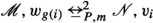
Given Lemma 4, for every 2-c-model ${\mathscr {M}}, w$, ${\mathscr {M}}_{{\textit{core}}}$ is partially functional, and . This means that, in showing the above claim, we can assume that ${\mathscr {M}}$ and ${\mathscr {N}}$ are partially functional. Now we show it by induction on k.

The base case is trivial. If ${\mathscr {M}}, w$ and ${\mathscr {N}}, v$ are partially functional 2-c-models such that , then we obtain ${\mathscr {T}}, u$ by setting ${\mathscr {T}} = \langle \{u\}, \{\}, V\rangle$ with V(u) agreeing with the valuation of w on $P \cup Q$ and the valuation of v on $P \cup R$, so that $V(u) \cap (P \cup Q) = V_{{\mathscr {M}}}(w)\cap (P \cup Q)$ and $V(u) \cap (P \cup R) = V_{{\mathscr {N}}}(v) \cap (P \cup R)$. Given that , this is doable.

For the inductive case, let ${\mathscr {M}}, w$ and ${\mathscr {N}}, v$ be partially functional 2-c-models such that . If w has no successor tuple, then we are back to the situation in the base case, so we deal with the case that w sees the tuple $\langle w_1, w_2\rangle$ and v sees the tuple $\langle v_1, v_2\rangle$ (v must have a successor tuple since ). Then, according to the definition of , we know that the following are true:

• there is a function $f:\{1, 2\}\rightarrow \{1, 2\}$ such that for $i \in \{1, 2\}$;

• there is a function $g:\{1, 2\}\rightarrow \{1, 2\}$ such that for $i \in \{1, 2\}$.

From this, we can show that there is a bijection $h:\{1, 2\}\rightarrow \{1, 2\}$ such that for $i \in \{1, 2\}$. If f is already injective, the let h be f. If f is not injective, let $j = f(1) = f(2)$. Then define h so that $h(g(3-j)) = 3-j$ and $h(3-g(3-j)) = j$, and it is not hard to check that it works.

With this h, we invoke I.H. to obtain ${\mathscr {T}}_1, u_1$ and ${\mathscr {T}}_2, u_2$ so that

Then, let ${\mathscr {T}}$ be the result of first taking disjoint union of ${\mathscr {T}}_1$ and ${\mathscr {T}}_2$, and then adding a point u with its valuation agreeing to that of w on $P\cup Q$ and to that of v on $P \cup R$, and then adding the triple $\langle u, u_1, u_2\rangle$ to the relation of ${\mathscr {T}}$. It is now easy to verify that

and we omit the routine details here. This completes the whole proof. $\square$

We conclude this section with three remarks. First, in the above proof, the existence of the bijection h corresponds to the following simple combinatoric fact: for any bipartite graph with the two parts each having exactly two vertices and each vertex’s degree is at least 1, there is a 2-edge covering of the 4 vertices. We can afford only 2 edges since we needed to create 2-models in which each point’s successor tuples can have at most 2 points. The same question can be asked for bipartite graphs where each part has $n > 2$ vertices: if the set of edges already covers every vertex, can we find a subcover with n edges? The answer is no. In fact, consider the graph $G = \langle V, E\rangle$ such that $V = \{a_1, b_1, a_2, b_2, \ldots , a_n, b_n\}$ and $E = \{\{a_1, b_i\} \mid i = 1, \ldots , n-1\} \cup \{\{a_i, b_n\} \mid i = 2, \ldots , n\}$. In picture, G is as follows:

Clearly, E covers V, but E has no proper subcover. Moreover, E has $2n-2$ many elements. When $n > 2$, $2n - 2 > n$. This shows why our proof above cannot extend to the case with $n > 2$. The number $2n-2$ of course is not necessary: so long as it is larger than n, it presents an obstacle to CIP. The importance of the above graph is that it is the worst case: for any bipartite graph where each part has n vertices and the edges cover the vertices, there must be a subcover of at most $2n-2$ edges.¹³ On the other hand, the counterexample we gave to the CIP of ${\mathbb {K}}_n$ for $n > 2$ in Example 5 realizes the graph in which V is still $\{a_1, b_1, a_2, b_2, \ldots , a_n, b_n\}$ but $E = \{\{a_1, b_1\}, \{a_1, b_2\}\} \cup \{\{a_i, b_j\} \mid i = 2, \ldots , n, j = 3, \ldots , n\}$. Any minimal subcover of this graph has $n+1 > n$ edges, and that is enough for the purpose of refuting CIP.

Second, note that the addition of ${\mathtt {C}}^{*}$ makes the $\Box$ a normal diamond in ${\mathbb {K}}_2{\mathtt {C}}^{*}$. Hence, if we interpret the $\Box$ by the diamond operation on Kripke frames, then ${\mathbb {K}}_2{\mathtt {C}}^{*}$ is precisely the logic of Kripke frames where each point has at most two successors, since now the axiom $\mathtt {K}_2 = (\Box p_1 \wedge \Box p_1 \wedge \Box p_2) \rightarrow \Box ((p_0 \wedge p_1) \vee (p_0 \wedge p_2) \vee (p_1 \wedge p_2))$ is logically equivalent to $(\Box p_1 \wedge \Box p_1 \wedge \Box p_2) \rightarrow (\Box (p_0 \wedge p_1) \vee \Box (p_0 \wedge p_2) \vee \Box (p_1 \wedge p_2))$ (by pushing the $\Box$, which is now a diamond operator, inside the disjunction), which is precisely the standard Sahqvist formula defining the frame property of each point having no more than two successors. This means that the logic ${\mathbb {K}}_2{\mathtt {C}}^{*}$ is precisely the logic ${\mathbb {K}}\mathtt {Alt}_2$ (using the notation in Segerberg 1971 and Kracht 1999) once we switch the role of $\Diamond$ and $\Box$. Hence, from the above theorem, we immediately obtain:

Corollary 2

${\mathbb {K}}\mathtt {Alt}_2$ has CIP, and ${\mathbb {K}}\mathtt {Alt}_n$ for any $n > 2$ lacks CIP.

Finally, instead of strengthening the logic, a restriction to the language may also lead to CIP. In particular, note that there does not seem to be an obvious way to reduce the number of distinct propositional letters in the examples we provided. In light of this, we leave the following question open:

Question 1

Is there an m for each n such that once $|\mathsf {Prop}| \le m$, ${\mathbb {K}}_n$ has the Craig Interpolation Property?

5 Conclusion

In this paper, we proved three results about $\textsf {WAML}$: first, $\textsf {WAML}$ have a van Benthem–Rosen characterization; second, basic $\textsf {WAML}$ systems do not have Craig Interpolation Property; and third, a special extension of ${\mathbb {K}}_{2}$ has CIP. We conclude with some potentially promising lines of further investigation.

First, we did not cover the usual infinitary constructions, such as ultrafilter extension, for $\textsf {WAML}$. Given the definition of canonical models in Apostoli and Brown (1995), Defintion 6.0) and the proofs therein, a definition of ultrafilter extension can be readily read off from it. A more direct and in fact also more general algebraic presentation is also in Urquhart (2009). However, we feel that the proofs there are very dense and also somewhat obscured by the general multi-ary modality setting. Thus, we believe it is worthwhile to have a simpler presentation of the ultrafilter extension, and we also believe that, contrary to what is done in Urquhart (2009), taking the dual $\Diamond$ of the weakly aggregative $\Box$ as the primitive will allow more elegant proofs (see Ding et al. 2021).

Second, the main part of the completeness proof of ${\mathbb {K}}_n$ over n-models in Nicholson et al. (2000) is to solve a combinatorial puzzle. Due to the semantics of $\textsf {WAML}$, there is a natural link between combinatorics and $\textsf {WAML}$ as also shown in the use of graph coloring problem in Apostoli and Brown (1995). As future work, we would like to explore the possibility of using $\textsf {WAML}$ to express interesting combinatorial properties in graphs, like the one in Nicholson and Allen (2003).

Third, even though we proved that basic $\textsf {WAML}$ systems do not have Craig Interpolation Property, it does not mean that the same must be the case for stronger logics, as we have already seen for ${\mathbb {K}}_{2}{\mathtt {C}}^{*}$. The counterexample in our paper cannot show that ${\mathbb {K}}_n\mathtt {T}$ lacks CIP since the logic is not sound on the frames of the models we provided. What remains to be done then is to chart the map of CIP among the logics extending ${\mathbb {K}}_n$’s and look for more general methods.

Lastly, as we observed in Corollary 2, it seems that, more abstractly speaking, the counterexamples exist because the logic can reason about, but cannot express directly, whether there are many accessible worlds satisfying a property, with the help of extra propositional letters. Note that counting the number of accessible worlds satisfying a property is intuitively important and has been studied in Description Logics (DL) (Baader et al. 2008) and Graded Modal Logics (GML) (Fine et al. 1972; Fattorosi-Barnaba and De Caro 1985; De Caro 1988). There are already some CIP work in those logics, like (Lutz and Wolter 2011), and we conjecture that CIP may return when we add modalities that talk directly about numbers.

References

Allen, M. (2005). Complexity results for logics of local reasoning and inconsistent belief. In Proceedings of the 10th conference on Theoretical aspects of rationality and knowledge (pp. 92–108). National University of Singapore.
Andréka, H., Németi, I., & van Benthem, J. (1998). Modal languages and bounded fragments of predicate logic. Journal of Philosophical Logic, 27(3), 217–274.
Andréka, H., Van Benthem, J., & Németi, I. (1995). Back and forth between modal logic and classical logic. Logic Journal of the IGPL, 3(5), 685–720.
Apostoli, P. (1997). On the completeness of first degree weakly aggregative modal logics. Journal of Philosophical Logic, 26(2), 169–180.
Apostoli, P., & Brown, B. (1995). A solution to the completeness problem for weakly aggregative modal logic. The Journal of Symbolic Logic, 60(3), 832–842.
Arló Costa, H. (2005). Non-adjunctive inference and classical modalities. Journal of Philosophical Logic, 34(5), 581–605.
Baader, F., Horrocks, I., & Sattler, U. (2008). Description logics. Foundations of Artificial Intelligence, 3, 135–179.
Beall, J., Brady, R., Dunn, J. M., Hazen, A. P., Mares, E., Meyer, R. K., Priest, G., Restall, G., Ripley, D., Slaney, J., & Sylvan, R. (2012). On the ternary relation and conditionality. Journal of Philosophical Logic, 41(3), 595–612.
Blackburn, P., De Rijke, M., & Venema, Y. (2002). Modal logic (Vol. 53). Cambridge University Press.
Blackburn, P., van Benthem, J. F., & Wolter, F. (2006). Handbook of modal logic (Vol. 3). Elsevier.
Chellas, B. F. (1980). Modal logic: An introduction. Cambridge University Press.
De Caro, F. (1988). Graded modalities, ii (canonical models). Studia Logica, 47(1), 1–10.
de Rijke, M. (1993). Extending modal logic. Ph.D. thesis, ILLC, University of Amsterdam.
Ding, Y., Liu, J., & Wang, Y. (2021). Hypergraphs, local reasoning, and weakly aggregative modal logic. In International workshop on logic, rationality and interaction (pp. 58–72). Springer.
Fagin, R., Halpern, J., Moses, Y., & Vardi, M. (1995). Reasoning about knowledge. MIT Press.
Fan, J., Wang, Y., & van Ditmarsch, H. (2015). Contingency and knowing whether. The Review of Symbolic Logic, 8, 75–107.
Fattorosi-Barnaba, M., & De Caro, F. (1985). Graded modalities. I. Studia Logica, 44(2), 197–221.
Feferman, S. (2008). Harmonious logic: Craig’s interpolation theorem and its descendants. Synthese, 164(3), 341–357.
Fervari, R., Herzig, A., Li, Y., & Wang, Y. (2017). Strategically knowing how. In Proceedings of IJCAI’17 (pp. 1031–1038).
Fine, K., et al. (1972). In so many possible worlds. Notre Dame Journal of formal logic, 13(4), 516–520.
Fusco, M. (2015). Deontic modality and the semantics of choice. Philosophers’ Imprint, 15.
Goranko, V., Otto, M., et al. (2007). Model theory of modal logic. Handbook of Modal Logic, 3, 249–329.
Gu, T., & Wang, Y. (2016). “knowing value” logic as a normal modal logic. In L. Beklemishev, S. Demri, & A. Máté (Eds.), Advances in modal logic (Vol. 11, pp. 362–381). College Publications.
Hansen, H., Kupke, C., & Pacuit, E. (2009). Neighbourhood structures: Bisimilarity and basic model theory. Logical Methods in Computer Science, 5(2)
Jennings, R. E., Johnston, D., & Schotch, P. K. (1980). Universal first-order definability in modal logic. Mathematical Logic Quarterly, 26(19–21), 327–330.
Jennings, R. E., & Schotch, P. K. (1981). Some remarks on (weakly) weak modal logics. Notre Dame Journal of Formal Logic, 22(4), 309–314.
Kamp, H. (1968). Tense logic and the theory of linear order. Ph.D. thesis, UCLA
Kracht, M. (1999). Tools and techniques in modal logic (Vol. 97). Elsevier.
Lewis, D. (1974). Intensional logics without interative axioms. Journal of Philosophical Logic, 3, 457–466.
Libkin, L. (2013). Elements of finite model theory. Springer.
Liu, J. (2019). Model theoretical aspects of normal polyadic modal logic: An exposition. Studies in Logic, 12(3), 79–101.
Liu, J., Wang, Y., & Ding, Y. (2019). Weakly aggregative modal logic: Characterization and interpolation. In Proceedings of the 7th international workshop on logic, rationality, and interaction (pp. 153–167). Springer.
Lutz, C., & Wolter, F. (2011). Foundations for uniform interpolation and forgetting in expressive description logics. In Twenty-second international joint conference on artificial intelligence.
Nicholson, D. (2009). A dualization of neighbourhood structures. In R. E. Jennings, P. K. Schotch, & B. Brown (Eds.), On Preserving: Essays on preservationism and paraconsistent logic (pp. 49–60). University of Toronto Press.
Nicholson, T., & Allen, M. (2003). Aggregative combinatorics: An introduction. In Proc. student session, 2nd North American summer school in logic, language, and information (NASSLLI-03) (pp. 15–25).
Nicholson, T., Jennings, R. E., & Sarenac, D. (2000). Revisiting completeness for the \({K}_{n}\) modal logics: A new proof. Logic Journal of IGPL, 8(1), 101–105.
Otto, M. (2004). Elementary proof of the van Benthem–Rosen characterisation theorem. Technical Report 2342.
Pattinson, D. (2013). The logic of exact covers: Completeness and uniform interpolation. In Proceedings of the 2013 28th annual ACM/IEEE symposium on logic in computer science (pp. 418–427). IEEE Computer Society.
Rosen, E. (1997). Modal logic over finite structures. Journal of Logic, Language and Information, 6(4), 427–439.
Routley, R., & Meyer, R. K. (1972). The semantics of entailment-II. Journal of Philosophical Logic, 1(1), 53–73.
Routley, R., & Meyer, R. K. (1972). The semantics of entailment-III. Journal of Philosophical Logic, 1(2), 192–208.
Santocanale, L., Venema, Y., et al. (2010). Uniform interpolation for monotone modal logic. In L. Beklemishev, V. Goranko, & V. Shehtman (Eds.), Advances in Modal Logic (Vol. 8, pp. 350–370). College Publications.
Schotch, P., & Jennings, R. (1980). Modal logic and the theory of modal aggregation. Philosophia, 9(2), 265–278.
Segerberg, K. (1971). An essay in classical modal logic. Filosofiska Föreningen Och Filosofiska Institutionen Vid Uppsala Universitet.
Seifan, F., Schröder, L., & Pattinson, D. (2017). Uniform interpolation in coalgebraic modal logic. In 7th Conference on algebra and coalgebra in computer science (CALCO 2017). Schloss Dagstuhl-Leibniz-Zentrum fuer Informatik.
Urquhart, A. (2009). Weakly additive algebras and a completeness problem. In R. E. Jennings, P. K. Schotch, & B. Brown (Eds.), On preserving: Essays on preservationism and paraconsistent logic (pp. 33–48). University of Toronto Press.
Van Benthem, J. (2008). The many faces of interpolation. Synthese, 451–460.
Van Benthem, J., Bezhanishvili, N., Enqvist, S., & Yu, J. (2017). Instantial neighbourhood logic. The Review of Symbolic Logic, 10(1), 116–144.
van Benthem, J., van Eijck, J., & Kooi, B. (2006). Logics of communication and change. Information and Computation, 204(11), 1620–1662.
Wang, Y. (2018). A logic of goal-directed knowing how. Synthese, 195(10), 4419–4439.
Wang, Y., & Fan, J. (2014). Conditionally knowing what. In R. Goré, B. P. Kooi, & A. Kurucz (Eds.), Advances in modal logic (Vol. 10, pp. 569–587). College Publications.
Author information
Authors and Affiliations
Corresponding author
Additional information
Publisher's Note
Springer Nature remains neutral with regard to jurisdictional claims in published maps and institutional affiliations.
This paper is an extended journal version of Liu et al. (2019). In this extended version, a detailed proof of Theorem 2 is provided using updated techniques, and a new result on recovering Craig interpolation (Theorem 6) is added. Jixin Liu thanks China Postdoctoral Science Foundation (2020M683344) and Fundamental Research Funds of SCU (2021-Philosophy-02) for support. Yanjing Wang gratefully acknowledges the support from NSSF (Grant 19BZX135).
Rights and permissions
About this article
Cite this article
Liu, J., Ding, Y. & Wang, Y. Model Theoretical Aspects of Weakly Aggregative Modal Logic. J of Log Lang and Inf 31, 261–286 (2022). https://doi.org/10.1007/s10849-022-09366-x
Accepted:
Published:
Issue Date:
DOI: https://doi.org/10.1007/s10849-022-09366-x