Distributed multi-agent scheduling and control system for robotic flexible assembly cells

Abstract

This paper deals with the development of a distributed multi-agent system (DMAS) for scheduling and controlling Robotic Flexible Assembly Cells (RFAC). In the proposed system, an approach for solving one of the most challenging decisional problems in RFAC is proposed and implemented. This problem is related to the products operations scheduling which requires their allocation and sequencing on the robots, while satisfying products and robots constraints under makespan minimization. The proposed DMAS addresses this challenge by using a cooperative approach supported by three kinds of autonomous control agents: supervisory agent, local agents, and remote agents. These agents interact by a negotiation protocol based on common dispatching rules for coordinating their individual decisions, satisfying their local objective and providing an optimized global solution. Moreover, because of the dynamic nature of the assembly systems, it is imperative to consider external disturbances on production scheduling and to solve the related issues. Consequently, DMAS has the ability to respond and manage some dynamic events that may occur in the cells such as unexpected robot breakdown or dynamic products arrivals. Computational results on benchmarks show the effectiveness and the robustness of the proposed system.

Introduction

Nowadays, with increasing global competition and responding to unpredictable demands, companies are forced to develop Flexible Manufacturing Systems (FMS) while benefiting from their ability to quickly minimize the required changes to produce new products, to support diversity of customers’ needs and their ability to deal with to unforeseen disruptive events. The most widespread class in the manufacturing industry is the Flexible Assembly Systems (FAS). In these systems, flexible assembly robots are used to perform assembly operations on families of products (Tang and Wong 2005). FAS are one of the most important areas in today’s industry; they offer a more consistent product quality, better repeatability, higher speed, consistent throughput, and better control. The use of industrial robots related to integrated planning and control in intelligent systems, allows FAS to accommodate the constant changes of their products and varying production volumes. Robots in FAS are able to quickly change their tools to perform a wide variety of repetitive tasks which allows these systems to change production quickly without having to reprogram anything or change equipment.

FAS can be divided into two main types (Sawik 1999): Robotic Assembly Line (RAL) and Robotic Flexible Assembly Cell (RFAC). RAL is a flow type system; it consists of a serie of special-purpose robotic assembly stations connected by an automated material handling system. However, RFAC is a highly modern system structured with industrial robots, assembly stations and an automated material handling; all are monitored by computer numerical control (Sawik 1999; Abd et al. 2014). In this paper, we are interested in RFAC, due to the advantages that offer over RFAL such as the ability to simultaneously mount a variety of products using the same resources, etc.

In RFAC where various types of products are assembled concurrently, the use of robots leads to increase productivity and reconfiguration capacity with minimal cost and robustness (Abd et al. 2014). The decision problems in FAS are classified as design, planning, scheduling, and control (Sawik 1999). The main focus of this paper is the scheduling and control problems in which an efficient FAS scheduling and control can manage the robots’ cooperation/coordination and improve their performances. The scheduling problem consists of finding the best way to use the cell robots as effectively as possible to allocate and sequence all the products. However, the objective of the controller is to monitor the overall system and taking the necessary corrective actions when dynamic disturbances occur.

There are several types of scheduling problems in the literature that differ according to the definition of their organization and their range. Because of their complexity, meta-heuristic algorithms are the most approximate methods used in the literature. They are able to solve large-scale NP-hard problems in less computational time compared to exact algorithms while arriving at high-quality near optimal solutions (Hosseini and Al Khaled 2014). These algorithms can be regrouped on two classes, (i) Algorithms based on neighborhood search that start from an initial solution and then the algorithm tries to improve it by choosing a new solution in the neighborhood, such as Tabu Search (TS) (González et al. 2013) and Adaptive Large Neighborhood Search (ALNS) (Vadlamani and Hosseini 2014). (ii) Algorithms based on global search which progressively improve a set of solutions (i.e. population) generated randomly, in general. Most of them are based on searching for many solutions by simple simultaneous calculation and then selecting the best one; such as Genetic Algorithm (GA) (Lu et al. 2015), Imperialist Competitive Algorithm (ICA) (Hosseini et al. 2014) and Particle Swarm Optimization (PSO) (AitZai et al. 2016).

The challenges on decision problems in FAS led researchers to develop control architectures composed of many independent behaviours that attempt to provide integral solutions for such problems. These systems can be classified into centralized, decentralized, and distributed control architectures. Recently, a great deal of effort has been spent on developing distributed control architecture due their reconfigurability, flexibility and to their capacity of high adaptation to requirements of modern manufacturing systems. In this category, researchers have identified the potential of Distributed Artificial Intelligence (DAI) in solving complex problem. In DAI, multi-agent systems (MAS) have received a considerable attention due to their autonomy, flexibility, fault tolerance, distributed nature and their aptitude to negotiate for conflicts problem resolution. These distributed systems can exchange information efficiently and their entities cooperate effectively in solving complexes problems.

In fact, the next generation of advanced manufacturing systems needs to incorporate more distributed control, machine (robots) and product flexibility (Ennigrou and Ghdira 2008). In this context, the MAS advantageous features in terms of decentralization of decisions, their ability to cope with dynamic changes (i.e. ability to handle dynamic nature of the manufacturing environments), modularity and also their potential to represent and run cooperative and distributed applications allow manufacturing organizations to overcome the needs and challenges of future industrial production systems.

MAS have been widely applied to solve scheduling problems by many researchers in the literature. For such problems, the multi-agent based approaches mainly include either (i) heuristic algorithm that uses some heuristic rules to negotiate with each other for solving the problems (Aydin 2012), or (ii) meta-heuristic algorithm that uses various strategies to iteratively search the optimal solution. Wang et al. (2003) proposed a multi-agent and distributed ruler-based approach to handle production scheduling in a machine shop. Kouider and Bouzouia (2012) proposed a distributed multi-agent scheduling system based on cooperative approach to solve static and dynamic scheduling problems. Maoudj et al. (2015) proposed a multi-agent architecture in which an approach for task allocation and scheduling for multi-robot systems is implemented. In this architecture, the agents negotiate and cooperate to allocate tasks to robots, and then schedule them on the robots using priority rules. Erol et al. (2012) developed a multi-agent based on-line system for scheduling machines and vehicles in a manufacturing system which operates under a decentralized control. While they did not take into account the machine flexibility, satisfactory results are obtained in dynamic manufacturing environments. An agent-based dynamic scheduling system is proposed by Sahin et al. (2015). Their system is based on a market oriented programming approach which makes use of negotiation as a problem solving strategy. The system is proposed for scheduling of flexible machine groups and material handling system working under a manufacturing dynamic environment. A multi-agent scheduling system for solving flexible job shop scheduling problem is presented by Wei and Dongmei (2012). Their system is inspired by the structure and negotiation strategies of the human immune system. Nouiri et al. (2015) developed two effective and distributed multi-agent PSO algorithms to solve the flexible job shop scheduling problem.

The cooperation between assembly robots in RFAS has been studied in the literature from multiple points of view. From the scheduling point of view, the challenge is always to have the appropriate algorithm capable for better solving this problem. In this context, few studies have been done on scheduling problems in RFAC; they can be categorized into three groups (Abd et al. 2014, 2010, 2013c): the first group applies heuristic methods (Lin et al. 1995; Abd et al. 2013a, b), the second uses the expert systems (Van Brussel et al. 1990), and the third investigates the simulation as an approach to solve the problem (Glibert et al. 1990).

This paper presents our ongoing efforts toward the development of a Distributed multi-agent system (DMAS) for RFAC control that allows entities to interact and cooperate with each other, to reliably and efficiently accomplish tasks. The overall behaviour of the proposed DMAS emerges through dynamic interactions of its agents behaviours, which provides RFAC control with important characteristics such as good scheduling, high robustness, quick response, extensibility and good expandability. DMAS consists of three kinds of autonomous and cooperative control agents: Supervisory agent, Local agents, and Remote agents. In dealing with scheduling problem, the proposed system distributes the computational tasks among its agents, where a local objective is defined for each agent (i) cost time minimization in the allocation step and (ii) idle time minimization in the sequencing step. For solving the problem, all agents cooperate and interact to satisfy their own local objective in order to generate a solution which optimizes the global objective (Makespan).

In multi-agent heuristic based algorithms, it is difficult to guarantee the quality of solution; whereas, multi-agent meta-heuristic algorithms are non-deterministic and need to spend more time than the heuristic algorithms to find out a high-quality solution (Xiong and Fu 2015). Therefore, these approaches lack of good trade-off between the convergence speed and solution quality. However, our proposed multi-agent decision-making approach is guided by distributed algorithms based on dispatching rules. Consequently, our approach is deterministic and requires low computational time to generate good solutions. Moreover, because of the dynamic nature of the current RFAC environments, the proposed control system is able to manage some dynamic events that can occur during the production process (urgent client orders arrivals, etc.) and to guarantee fault-tolerance to unexpected robot breakdowns. This ability allows the system to continue working while absorbing these disturbing events (guaranteeing thus a minimal service).

The remainder of this paper is structured as follows. Second section describes the distributed multi-agent system proposed for scheduling and controlling RFAC. Third section presents the proposed mathematical model of the studied problem. Fourth section deals with the interaction process during the problem resolution; this section gives also an illustrative example. Fifth section validates the proposed approach via some benchmark instances of the literature. Finally, last section concludes the paper and gives future works.

The proposed scheduling and control system

Generally, modern RFAC consists of flexible conveyor system as transportation device, multiple industrial robots controlled by embedded-computers, and integrates Radio Frequency Identification (RFID) system which enables real-time information about products in the cells. The overall cell is monitored by of a set of interconnected computers and PLCs that allow management of the cell orders. Therefore, to make our DMAS generic and easily adapted to any RFAC by implementing only some new required modules (used in other flexible manufacturing systems integrating machines and robots), the proposed DMAS is distributed on two sides as described in Fig. 1: Decisional side (Planning level) and Physical side (Operative level), in which three kinds of autonomous agents (software applications) are implemented: Supervisory agent (SA), Local Agent (LA) and Remote Agent (RA). The last two kinds of agents are associated for each robot (resp. machine) in the cell. LAs make all decisions in planning and scheduling stages, to generate the scheduled local plans (sequenced assembly operations) ready for sending to their corresponding RA (for execution). RA is implemented on the robot control station (embedded-computer); it executes the scheduled local plan. All the agents are organized in a distributed manner and cooperate by exchanging messages to manage their interactions (Maoudj et al. 2015, 2016).

Fig. 1

The proposed DMAS for RFAC scheduling and control

Decisional side (planning level)

In RFAC, each robot is controlled by an embedded-computer, the overall cell is monitored by a supervision station (res. by many interconnected computers) connected to robots embedded-computers, the conveyor movement and RFID reader are controlled by PLCs. In DMAS, the decisional side gathers SA and LAs; they are installed on the supervision station (resp. the interconnected computers). These agents are responsible of global cell configuration, planning, scheduling and control. They collect parts and robots states and provides real-time monitoring of the cell. As we are only interested by scheduling problem in RFAC, we focus on the agents role in the problem solving.

Supervisory agent (SA)

This agent allows operators to manage and interact with the overall DMAS. SA is installed on the supervision station, it receives information about the initial cell parameters and products defined by a sequence of assembly operations. While implementing the necessary modules, SA can also connect to the PLCs that control the conveyor and the RFID system to control them and exchange data related to assembly part with LAs. In the scheduling process, SA does not take part in the decision-making phase for operations allocation; its main role is to dispatch operations onto LAs, which are in charge to perform such a decision.

Local agents (LAs)

LAs contain all needed modules to cooperate between them for operations allocation and local plans sequencing. Moreover, each LA obtains feedbacks from its corresponding RA (Failure notification, information sensors, information about operation execution progress, reports/ratios, etc.) and displays them on its user interface.

Physical side (operative level)

This side contains the physical robots system (i.e. the industrial robots cell). Each robot is controlled by a reactive RA implemented on its embedded computer. The main role of RA consists of carrying out the scheduled operations plans sent by its corresponding LA. In parallel, to obtain the robots state in real-time, RA sends all robot’s sensors information to LA during the execution process.

The scheduling problem in robotic flexible assembly cell

Let’s consider a RFAC composed of m industrial robots with n products to be realized. The considered scheduling problem is described as follows. There are a set of n independent products (jobs) $J=\{j_{1}, j_{2},...,j_{n}\}$, to be processed on m industrial robots $R=\{R_{1}, R_{2},..., R_{m}\}$. Each job $j_{i}$ consists of an ordered set of $n_{i}$ non preemptive assembly operations $\{O_{i1}, O_{i2},..., O_{i,n_{i}}\}$. Each assembly operation $O_{ij}$ (j th operation of job i) must be processed on one and only one robot among the set of robots R. In addition, at a given time, a robot can execute at most one operation. The aim is to find the best robots assignment to assembly operations and sequence them on each robot, while satisfying the operations precedence constraints and the disjunctive constraints on each robot under the minimization of the makespan $C_{max}$. This corresponds to the completion time of the last scheduled product (i.e. the maximal completion time of products), $C_{max}=\underset{i=1\dots n}{\mathrm {max}}{C}_{i}$ where $C_i$ represents the completion time of product $j_{i}$.

This problem is mathematically modeled by the Mixed Integer Linear Program (MILP) proposed bellow. The following notations describe indices, parameters and decision variables used in the developed model.

Parameters and indices

n :

Number of products (jobs).

m :

Number of industrial robots.

$n_{i}$ :

Total number of assembly operations in job i.

i, k:

Indices of jobs $i, k \in \{1,\ldots ,n\}$.

j, l:

Indices of operation order in a job $j, l \in \{1,\ldots ,n_{i}\}$.

r :

Index of robots $r\in \{1,\ldots ,m\}$.

$p_{ij,k}$ :

Processing time of the jth operation of job i on robot k.

M :

A large positive number.

$O_{i,j}$ :

The jth operation of job i.

Decision variables

$t_{ij}$ :

Start time of the jth operation of job i.

$C_{max}$ :

Makespan of a schedule.

$$\begin{aligned}&B_{ij,kl,r}\\&\quad = \left\{ \begin{array}{ll} 1, &{}\quad \hbox {if\;operation} O_{ij} \hbox {is\;performed\;before} O_{kl} \text { on robot } r,\\ 0, &{}\quad \hbox {otherwise.} \end{array}\right. \end{aligned}$$

$$\begin{aligned} A_{ij,r} = \left\{ \begin{array}{ll} 1, &{} \quad \hbox {if\;operation} O_{ij} \text { is assigned to robot } r, \\ 0, &{} \quad \hbox {otherwise.} \end{array} \right. \end{aligned}$$

The MILP is given as follows:

The objective function (1) consists of the makespan minimization.

$$\begin{aligned} Minimize \{C_{max}\} \end{aligned}$$

(1)

subject to:

Constraints (2) impose for the last operation of each job to be less than or equal to the makespan:

(2)

Constraints (3) ensure that the precedence relationships between the operations of a job are not violated, i.e. operation $O_{ij}$ is not started before operation $O_{i,j-1}$ has been completed.

(3)

Constraints (4) make sure that operation $O_{ij}$ is assigned to only one robot.

$$\begin{aligned}&\sum _{r=1}^m A_{ij,r} = 1\nonumber \\&\quad \forall i\in \{1,\ldots ,n\}, \forall j\in \{1,\ldots ,n_{i}\}, \quad \forall r\in \{1,\ldots ,m\}\nonumber \\ \end{aligned}$$

(4)

Constraints (5) and (6) enforce each robot to process at most one operation at a time.

(5)

$$\begin{aligned}&\sum _{r=1}^m (B_{ij,kl,r} + B_{kl,ij,r} - A_{ij,r}) = 0\nonumber \\&\quad \forall i,k \in \{1,\ldots ,n\}, \forall j,l \in \{1,\ldots ,n_{i}\}, \quad \forall r\in \{1,\ldots ,m\}\nonumber \\ \end{aligned}$$

(6)

Finally, constraint (7) require all t variables to be positive and constraints (8) require all B and A variables to be binary.

$$\begin{aligned} t_{ij} \ge 0 \quad \forall i \in \{1,\ldots ,n\}, \quad \forall j\in \{1,\ldots ,n_{i}\} \end{aligned}$$

(7)

$$\begin{aligned}&B_{ij,kl,r}\in \{0, 1\}, A_{ij,kl,r}\in \{0, 1\}\nonumber \\&\quad \forall i,k \in \{1,.., n\}, \forall j,l \in \{1,\ldots ,n_{i}\}, \forall r\in \{1,\ldots ,m\}\nonumber \\ \end{aligned}$$

(8)

The proposed scheduling approach

The problem described above can be divided into two closely related subproblems (i) allocating each assembly operation to a robot, and (ii) sequencing the assigned operations on each robot while satisfying the products constraints and minimizing the makespan. This problem can be seen as a Flexible Job Shop Scheduling Problem (FJSSP) (Maoudj et al. 2016; Park and Wang 2009) which is known to be NP-hard.

Because of the high complexity of this problem, its optimal resolution requires a very high computation time. Hence, the need to use heuristics or meta-heuristics (GA, PSO, TS, etc.) arises to achieve an approximate optimal solution. Most of these approaches are non-deterministic, centralized and require a huge computational time when the problem size increases. Consequently, to overcome these problems, the proposed DMAS approach only considers dispatching rules; this makes our approach deterministic and requires low computational time to generate the solutions.

The proposed system distributes the computational tasks among its agents. Each agent only completes a part of the computational tasks with lack of a full global view. For solving the problem, all agents interact and collaborate to satisfy both local and global objectives. The interaction in the proposed DMAS consists of the dynamic relations between the LAs through an interchanged set of actions (local information, exchange of messages, etc.). This setting of dynamic relationship between the LAs of the system led to a convergence toward a good solution.

Owing to the complexity of the problem and in order to make proper decisions resulting from interactions between the agents, two rules (GBPT and SBPT) are used in the allocation phase and combined with two other well-known rules (SRT and SPT) to sequence the allocated operations:

• Greatest Best Processing Time (GBPT) it selects operation with maximum BPT.

• Smallest Best Processing Time (SBPT) it selects operation with minimum BPT.

• Smallest Processing Time (SPT) it selects operation with minimum processing time.

• Smallest Release Time (SRT) it selects operation with minimum release time.

where, Best Processing Time (BPT) is the smallest processing time of the operation among their several processing times on the cell robots (as each assembly operation has the possibility to be processed by more than one robot).

Fig. 2

The proposed distributed resolution method for scheduling problem

Each agent has its own local objective in each resolution step (allocation and sequencing); each agent bases its decisions on the rules described above to minimize its local objective. Finally, the global solution is the result of the interactions between all the agents. The defined agents local objective is summarized as follows:

• Cost time minimizationin the allocation step to allocate an operation, the agent having the minimal cost holds the proposed operation. Let us consider $Cost_{ij,r}$ be the cost of operation $O_{ij}$ on robot r calculated by Eq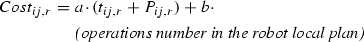. (9):

  

  (9)

  where a and b are two constant weights fixed by using preliminary tests.

• Minimization of robot idle time in the sequencing step let’s consider $r_{i}$ (resp. $c_{i}$) be the release time (resp. completion time) of the sequenced operation in the position i on a robot local plan. The idle time ($I_{i}$) of robot having an operation scheduled in position i is depicted in Eq. (10):

  $$\begin{aligned} I_{i} = \left\{ \begin{array}{ll} r_{i}-c_{i-1}, &{} \quad \hbox {if} \quad i>1\\ r_{i}, &{} \quad \hbox {if}\quad i=1\end{array}\right. \end{aligned}$$

  (10)

Interaction mechanism

The proposed distributed resolution method for scheduling problem is summarized in Fig. 2. Three distributed algorithms (Alg1, Alg2 and Alg3) are used in the interaction process in both allocation and sequencing steps. For this propose, SA receives jobs (products) data. After the system configuration, SA sends them to all concerned agents. Then, it builds Priority Matrix (PM) in which the operations are classified according to their priority level (to define which operation SA selects to dispatch it to LAs):

In PM, SA adds a priority level for each operation, given by its assigned row in PM: Operations of row 1 have priority 1, operations of row 2 have priority 2, until the last row. For example, let $h = MAX n_{i} (i\in \{1,\ldots ,n \})$, $J_{1}=\{O_{11}, O_{12},\ldots , O_{1n_{1}}\}$ be $Job_{1}$ that consists of a predetermined sequence of $n_{1}$ assembly operations to be consecutively processed. SA adds $O_{11}$ in level $L_{1}$ (row 1), $O_{12}$ in level $L_{2}$ (row 2)...$O_{1n_{1}}$ in level $L_{n_{1}}$ (row $n_{1}$), and so on for the other assembly operations of jobs $J_{2}$...$J_{n}$.

$$\begin{aligned} PM = \left[ \begin{array}{ccc} O_{11} &{} \quad \cdots &{}\quad O_{n1} \\ :&{}\quad \ddots &{}\quad :\\ O_{1h} &{} \quad \cdots &{} \quad O_{nh} \end{array} \right] \end{aligned}$$

In each priority level (each row in PM), the level operations are sequenced by using Alg1 as detailed by Fig. 3. Then, SA uses the obtained order to dispatch these operations one by one to LAs. In the decision-making process, SA considers the following rules in Algo1:

Fig. 3

Functional diagram of SA in the resolution process (Alg1)

• 1. In the first level ($L_{1}$), operations are ordered by using GBPT rule. We point out that the operation processing time is unknown, SA requests this time form LAs by exchanging messages.

• 2. For each level $L_{j}$$(1<j<h)$, if the number of products is more than 10, operations are ordered by using GBPT; otherwise, they are ordered by using SRT.

• 3. In GBPT rule, if GBPT values for some operations are equal, the operation that can be executed by only one robot has the priority. In case of another equality of GBPT, the operation having greatest number of successors that should be executed by one and only one robot will get the priority. If there is another equality of this last number, the order will be kept as it is.

• 4. In SRT rule, if more than one operation has the same SRT value, the operations are ordered by using SBPT rule. If there is an equality of SBPT, the operation that is executed by only one robot will get the priority. If an equality exists again, the operation having the greatest number of successors that should be executed by one and only one robot will get the priority. If the equality always persists, the order will be kept as it was.

The dispatching process of Alg1 is summarized below:

Step 1

• $h={\text{ max }}$$n_{i}$, number of the levels in PM

• For (all operations in level $L_{1}$), release times $=$ 0

• Order this level using GBPT rule

• $j=1$

• Goto Step 2

Step 2

• Dispatch operations of level $L_{j}$

• $j=j+1$

• Goto Step 3

Step 3

If ($j\le h$) then

• Wait for a message, which contains release times of operations in level $L_{j}$

• Goto Step 5

Else (i.e. all PM operations are allocated) Goto Step 6

Step 4

• Order operations of $L_{j}$ level by using SRT or GBPT rule

• Goto Step 2

Step 5

• Update the release time of the concerned operation in level $L_{j}$

• If (all release times are updated), Goto Step 4

• Else, Goto Step 3

Step 6

• Send a message to inform LAs that all the operations have been allocated to robots.

• End

Fig. 4

Functional diagram of LA in the resolution process

The decision-making process and the behaviour of each LA during the operations allocation are described in the functional diagram of Fig. 4 (Alg2):

• If sender is SA, three possible cases are distinguished:

  • 1. When the received message is about system configuration LA updates its database.

  • 2. When the received message is about an operation allocation If SA requests its processing time, LA responds by giving the requested information. Otherwise, LA evaluates its local cost to execute this operation and sends it within other useful information (allocated operations number, idle time on its local plan) to the other LAs.

  • 3. If the message is about the ending of planning process (all operations are allocated and sequenced) in this case, LA sends the final scheduled plan to SA.

• If sender is LA, two possible cases are distinguished:

  • 1. When the received message is about a cost proposition for an allocated operation The agent checks if all propositions (of its acquaintances) are received; in such a case, it compares them with its local cost. The agent that proposed the smallest cost will get the operation. If two agents or more give the same cost, the agent having the smallest number of allocated operations in its local plan will get the operation. If there is another equality of allocated operations number, the agent having the greatest idle time will get the operation. Afterwards, the agent that holds the operation adds it to its local plan and activates the sequencing process (Alg 3). Finally, LA sends its decision to SA informing it that the operation is allocated.

  • 2. When the received message is about the release time of an operation The agent re-sequences its local plan only if this operation is assigned to the current agent with a modified release time. Otherwise, the agent ignores the message.

The sequencing process is detailed in the flowchart of Fig. 5 (Alg3). We point out that in LAs local plan the operations have the same levels as in PM. For each level, operations with known release times are sequenced using SRT rule. If there is equality of the release times (for example, in level $L_{1}$ all operations release times are equal to zero), operations are sequenced using SPT rule. If there is also an equality of SPT, the first allocated will have the priority.

Fig. 5

Scheduling algorithm for LAs

The sequencing algorithm (Alg3) executed by LAs to sequence m level in their local plan is summarizes below:

Step 1

• $j=1$

• b = number of levels in the local plan $(b\in \{1,\ldots ,h\})$

• Goto Step 4

Step 2

• Update the release time of the concerned operation in level $L_{j}$

• If (all release times are updated) then Goto Step 4

• Else, Goto Step 3

Step 3

If ($j\le b$) then

• If (all release times of $L_{j}$ operations are updated) then Goto Step 4

• Else, wait for a message, which contains release times of operations in $L_{j}$

• Goto Step 2

Else (all operations of LA local plan are scheduled) Go to Step 5

Step 4

• Sequence the level $L_{j}$ operations by using SRT and SPT rules

• Send completion times of the scheduled operations to SA and all LAs, to inform them about the release times of their successors in the next level

• $j=j+1$

• Goto Step 3

Step 5

• End.

Rescheduling strategy in case of dynamic disturbances

In RFAC, some dynamic disturbances may occur during the assembly process, such as unexpected robots breakdown or new jobs (products) arrival. To provide a reliable fault-tolerant control system, disturbances mustn’t completely block the global RFAC.

A good scheduling algorithm not only allows obtaining high-quality scheduling solutions, but can flexibly and quickly respond to dynamic disturbances during production (assembly) process. However, many agent-based approaches of the literature lack of these two characteristics in the same time. Fortunately, our DMAS offers both of these properties; the agents reaction to these disturbing events are detailed below:

• 1. Case of robot breakdown RA of the broken robot (i.e. reactive agent implemented on robot embedded computer) informs its corresponding LA about this problem. Subsequently, LA informs all the other LAs about its unavailability, and rejects all its assembly operations. Next, LA sends its operations to SA. Afterwards, the other LAs send their operations that are not executed yet to SA. After that, SA removes the executed (resp. in progress) operations from the last ordered levels (in PM) that are saved in its database. Finally, the same interaction process explained previously is repeated in order to reassign and re-sequence the operations of the new PM.

• 2. Case of new job arrival SA reacts to this disturbance by informing all LAs about the new job arrival; after that, each LA responds by sending information about its un-executed operations. Afterwards, SA constructs a new PM in which it adds the new job, then orders the PM levels as explained above. Finally, the same procedures are repeated to allocate and sequence all operations.

Illustrative example

In this subsection, we present an example to clarify the interactions between the agents to solve static and dynamic scheduling problems. For both cases, we consider an example of five (05) robots working in a RFAC to carry out four (04) products (jobs). Each product consists of three assembly operations. In addition, each robot is able to carry out all these operations. The problem presented in Table 1 is deduced from Kacem $4\times 5$ FJSSP benchmark (Kacem et al. 2002), which is an instance of 04 jobs and 05 machines.

Table 1 Operations processing times on each robot (deduced from $4\times 5$ Kacem instance)

Table 2 Scheduled local plan of the LAs after each operation allocation

Fig. 6

Gantt diagram of the obtained solution

Scheduling strategy in static cases

We assign to each robot a local agent (i.e. LA1, LA2, LA3, LA4 and LA5). SA starts by building PM as detailed previously:

$$\begin{aligned} PM=\left[ \begin{array}{cccc} O_{11}(BPT_{R4}=1) &{} O_{21}(BPT_{R1}=2)&{} O_{31}(BPT_{R3}=6) &{} O_{41}(BPT_{R4}=1) \\ O_{12}(BPT_{R2}=4) &{} O_{22}(BPT_{R1,R5}=5)&{} O_{32}(BPT_{R2}=1) &{} O_{42}(BPT_{R1}=1) \\ O_{13}(BPT_{R1,R4}=4) &{} O_{23}(BPT_{R1,R3}=4)&{} O_{33}(BPT_{R1,R4}=2) &{} O_{43}(BPT_{R2,R4}=1) \end{array} \right] \end{aligned}$$

where $BPT_{Ri}$ means that the Best Processing Time (BPT) is given by $LA_{i}$ on robot $R_{i}$, $i\in \{1,\ldots ,5\}$.

To sequence PM levels, SA orders the levels by using the proposed rules then dispatches the levels operations one by one as detailed above. For the first level $L_{1}$, the ordered given by the proposed rules is {$O_{31}$$O_{21}$$O_{11}$$O_{41}$}.

In the following, we note SLP as a Scheduled Local Plan of an agent. Table 2 summarizes all the ordered levels ($L_{1}$, $L_{2}$ and $L_{3}$). For each operation allocation, the concerned LA sequences its local plan then sends the completion times of all operations to the other LAs (symbol $>>$ denotes succession between operations on the agents SLP).

The final solution is represented by Fig. 6. The obtained solution has a makespan of 11; this represents the optimal solution.

Rescheduling strategy in dynamic cases

As a second test, we consider the occurrence of some unexpected disturbances during the production process. Consequently, to show the robustness of the DMAS and how it reacts and manages these disturbing events, two cases are considered:

Table 3 The new information (state of the robots) at T$=$1 s

Fig. 7

Gantt diagram of the new solutions (left) when a robot breaks at $T=1$ s, (right) when a new job arrives at $T=2$ s

• Robot breakdown We assume that during the execution process, robot $R_4$ (i.e. LA4) breaks down at time $T=1$ s. Table 3 summarizes the state of the robotic cell at this time. After the rescheduling process, the new solution obtained is depicted by Fig. 7 (left) in form of Gantt diagram.

• A new job arrives Another disturbance event is considered; we assume that at $T=2$ s a new job $J_5$ arrives (it is a customer order). Table 4 shows the processing time of the assembly operations on the cell robots.

SA reacts to this disturbance by informing all LAs about the new job arrival; after that, each LA responds by sending information about its un-executed assembly operations. Afterwards, SA constructs a new PM in which it adds the new job ($J_5$), then orders the PM levels as explained above. Finally, the same procedures are repeated to allocate and sequence all operations. The obtained rescheduled plan is given in Fig. 7 (right).

It can be seen that the reactivity of the proposed DMAS to cell disturbances is high; the unavailability (failure) of an agent (i.e. a robot) or the arrival of new job did not affect/block the other agents/overall system.

Computational validation results

DMAS has been implemented using C# which is one of the powerful object-oriented programming languages. The agents are implemented as autonomous software applications which interact through exchanging of messages via TCP/IP protocol. The choice of C# is mainly based on its features related to events and delegations.

Table 4 The new job operations processing times on the robots

To test the performances and effectiveness of the proposed scheduling approach, some FJSSP benchmark instances have been considered. For each machine of a benchmark problem, an autonomous LA is associated which interacts with its acquaintances through messages exchange. In order to make comparisons with literature works, we enforce each robotic agent (LA) to evaluate the processing time of each of its assembly operations as given in the tested benchmark.

The weights a and b used in Eq. (9) are fixed empirically by using preliminary experiments to 0.9 and 0.1, respectively. In addition, for all the computational experiments, the agents run on a host PC with 1.90 GHz Core i3 CPU and 4 GB RAM.

The proposed approach solutions are compared in terms of solution quality by using two sets of FJSSP (Fattahi and Brandimarte benchmarks). The solutions are also compared in terms of solution quality and computational time by using Kacem benchmarks:

• Ten instances of Fattahi benchmarks (Fattahi et al. 2007) SFJS1–SFJS10.

• Ten instances of Brandimarte benchmarks (Brandimarte 1993) MK01–MK10.

• Four instances of Kacem benchmarks (Kacem et al. 2002) ($4\times 5$), ($8\times 8$), ($10\times 10$), ($15\times 10$).

For performances evaluation, our approach is compared with: (i) centralized approaches by using Fattahi benchmarks, (ii) distributed approaches by using Brandimarte benchmarks, and (iii) with both types by using Kacem benchmarks.

Table 5 Computational results of DMAS on Fattahi instances compared with ITS and ISA

Table 6 Computational results on Brandimarte instances

Comparison with centralized approaches using Fattahi benchmarks

We compare with three algorithms proposed by Fattahi et al. (2007): ISA (Integrated approach with Simulated Annealing heuristic), ITS (Integrated approach with Tabu Search heuristic) and HTS/SA (algorithm use Hierarchical approach and TS heuristic for assignment problem and SA heuristic for sequencing problem). Results are presented in Table 5; columns 1 and 2 represent the problem name and its lower bound, respectively. Columns 3, 6 and 9 represent the average makespan obtained by 10 runs of the same instance for ITS, ISA and HTS/SA algorithms, respectively. Columns 4, 7 and 10 represent the best found solution for ITS, ISA and HTS/SA algorithms, respectively. Columns 5, 8 and 11 represent the Df value, where Df determines the mean deviation of the best solution; it is given by (11) where $n=10$ runs, and $f^{*}$ denotes the best solution obtained by the mathematical model proposed in Fattahi et al. (2007). The last two columns refer to the makespan and Df obtained by our proposed DMAS.

$$\begin{aligned} Df =\sum _{i=1}^n (f_{i}-f^{*})/n.f^{*} \end{aligned}$$

(11)

Table 7 Comparison between makespan and CPU execution times of PSO, NIMASS, LEGA and DMAS

As the proposed DMAS is deterministic, Df is evaluated by (12):

$$\begin{aligned} Df =(C_{max} - f^{*}) / f^{*}. \end{aligned}$$

(12)

Comparison with distributed approaches using Brandimarte benchmarks

The comparison with purely distributed agent-based approaches FJS MATSLO (Multi-Agent Tabu Search Local Optimization), FJS MATSLO+ (Ennigrou and Ghdira 2008; Henchiri et al. 2013) (where each problem is carried out 5 times) and DMAPRGA (Distributed Multi-agent Approach based on Priority Rules and Genetic Algorithm) (Maoudj et al. 2016) is given in Table 6. The problem names are listed in the first column, the second column refers to the $C_{max}$ of the solution given by FJS MATSLO. The third column stands for the $C_{max}$ of the solution given by FJS MATSLO+. The fourth column presents the $C_{max}$ of the solution given by DMAPRGA. The last column shows the $C_{max}$ of the solution obtained by the proposed DMAS.

Fig. 8

CPU processing times of PSO, NIMASS, LEGA and DMAS

Comparison with centralized and distributed approaches using Kacem benchmarks

A good scheduling algorithm is not only able to generate high-quality scheduling solution, but it must quickly obtain this solution (good convergence speed). However, many approaches in the literature lack of good compromise between the convergence speed and solution quality. Therefore, as another test, the effectiveness of DMAS is analyzed in terms of CPU time (convergence speed). For this purpose, obtained results for Kacem instances (2002) are compared with those of some published approaches using meta-heuristic algorithms:

• A new immune multi-agent system for the flexible job shop Scheduling problem (NIMASS) It is run on 2GB RAM and on PC with 2.1 GHz CPU (Xiong and Fu 2015).

• Multi-Agent Particle Swarm Optimization (PSO) Carried out on Intel Core2Duo 2.0 GHz and having 3070 MO of memory (Nouiri et al. 2015).

• LEarnable Genetic Architecture (LEGA) It is run on Pentium IV with 2.0 GHz (Nhu Binh et al. 2007).

Table 7 shows the makespan and CPU execution time (in seconds) of each approach. The last two columns show makespan and CPU execution time obtained by our DMAS approach, respectively. Figure 8 shows CPU execution times of the compared approaches.

Discussion of obtained results

As it can be seen in Table 5, obtained results show that DMAS finds the optimal solution for 06 instances among 10. Whereas, ISA, ITS and HTS/SA reach the optimal solutions for 06, 09 and 09 instances, respectively. Furthermore, for the near optimal solutions DMAS has an average (i.e. Df) equal to 0.12 which attests the good quality of these near solutions.

Table 6 gives a comparison between our DMAS and the other distributed multi-agent based approaches. In comparison with DMAPRGA, DMAS has better results for MK02, MK03, MK04 and MK05; the same result is obtained for MK01. As it is shown in Table 6, the obtained results by DMAS for MK02, MK05, MK06, MK09 and MK10 instances are batter than those obtained by FJS MATSLO+. Whereas, DMAS achieved better results only for MK02 and MK10 and same result for MK01 compared with FJS MATSLO. On the basis of the non-deterministic and the fact that meta-heuristic based approaches require much computational CPU time, we can see that the quality of the near optimal solution given by DMAS is generally high. Despite the fact that DMAS is deterministic, distributed, based on non-global information and uses only four rules in the scheduling process, it gives good results (optimal or near-optimal solutions) which are close enough to results given by non-deterministic and centralized approaches that use global information.

From the results shown in Table 7, the interactions between agents allow to quickly converge toward a good solution (i.e. best or near-best solution). For $(4 \times 5)$ instance, DMAS generated the best makespan (i.e. 11) in 0.05 s while PSO and NIMASS converged to the best makespan in 0.35 and 1.2 s, respectively. For the other $(8 \times 8)$, $(10 \times 10)$ and $(15 \times 10)$ instances, the results given by DMAS are near to the best solutions with best CPU time. For all these reasons (CPU times and obtained makespan values), we can attest that results given by DMAS are very satisfactory.

Moreover, the quality of solutions obtained by meta-heuristic based algorithms strongly depends on the quality of initial solution and the settings of many parameters. In addition, initializing such parameters is very difficult in the real production process with various dynamic disturbances (Xiong and Fu 2015); this gives another reason to prove the good performances of our proposed DMAS since it has no parameter to be determined.

There are other several reasons to substantiate the good performances of the proposed DMAS. First, DMAS is generic, modular, flexible and reconfigurable (it has the ability to adapt to the changes in the cell environment). Second, the agents in DMAS are autonomous, independent and use local information by exploring a purely distributed approach through no master/slave relationship between the decisional agents. Third, DMAS is robust; it reacts and manages dynamic disturbances. Indeed, the agents are capable of making real-time decisions depending on the robots state in any unplanned or unforeseen events without needing any specific additional treatment. Finally, our proposed agent-based approach combines only four heuristic rules that allows obtaining a good balance between computational time and quality of solutions which is the main drawback of many approaches in the literature.

Conclusion and future work

In this paper, we have presented a distributed multi-agent control system (DMAS) for robotic flexible assembly cells. In this system, we discuss one of the most challenging decisional problems which is the scheduling problem. For this purpose, a distributed approach while using dispatching rules has been described and implemented. In DMAS, agents solve sub-problems locally to propose a global solution as a result of interactions between the different agents. The problem resolution is mainly done in two phases: (i) Allocation and (ii) Sequencing. In each phase, the agents interact and cooperate to satisfy their local objectives, i.e. cost time minimization in allocation phase and idle time minimization in sequencing phase, to quickly converge to the global objective (Makespan minimization). In the interaction process, the agents decisions are made while using and combining only four dispatching rules (GBPT, SBPT, SPT and SRT).

The agents cooperate by exchanging messages to locally produce a feasible scheduled local plan; this is done in order to converge at best toward a global solution that minimizes the makespan.

Comparisons with literature works, by using FJSSP benchmarks, show the effectiveness of the proposed DMAS. In addition, other features of the system have been tested and discussed such as the ability to manage some dynamic events (such as new products arrivals) and fault-tolerance to robots failures. If an agent (robot) breakdowns, the system may still working without adding any specific treatment.

Future works will consider the bi-objective optimization, including the most known objectives in scheduling problems: the Makespan ($C_{max}$) and the sum of total completion time ($\sum _{i=1}^n C_i$).

References

Abd, K., Abhary, K., & Marian, R. (2010). A Scheduling framework for robotic flexible assembly cells. AIJSTPME Asian International Journal of Science and Technology in Production and Manufacturing Engineering, 4(1), 30–37.
Abd, K., Abhary, K., & Marian, R. (2013a). Application of fuzzy logic to multi-objective scheduling problems in robotic flexible assembly cells. Automation Control and Intelligent Systems, 1(3), 34–41.
Abd, K., Abhary, K., & Marian, R. (2013b). Fuzzy decision support system for selecting the optimal scheduling rule in robotic flexible assembly cells. Australian Journal Of Multi-Disciplinary Engineering, 9(2), 125–132.
Abd, K., Abhary, K., & Marian, R. (2013c). A scheduling framework for robotic flexible assembly cells, KMUTNB: International. Journal of Applied Science and Technology, 4(1), 31–38.
Abd, K., Abhary, K., & Marian, R. (2014). Simulation modelling and analysis of scheduling in robotic flexible assembly cells using Taguchi method. International Journal of Production Research, 52(12), 2654–2666.
AitZai, A., Benmedjdoub, B., & Boudhar, M. (2016). Branch-and-bound and PSO algorithms for no-wait job shop scheduling. Journal of Intelligent Manufacturing, 27(3), 679–688.
Aydin, M. E. (2012). Coordinating metaheuristic agents with swarm intelligence. Journal of Intelligent Manufacturing, 23(4), 991–999.
Brandimarte, P. (1993). Routing and scheduling in a flexible job shop by tabu search. Annals of Operations research, 41(3), 157–183.
Ennigrou, M., & Ghdira, K. (2008). New local diversification techniques for flexible job shop scheduling problem with a multi-agent approach. Autonomous Agents and Multi-Agent Systems, 17(2), 270–287.
Erol, R., Sahin, C., Baykasoglu, A., & Kaplanoglu, V. (2012). A multi-agent based approach to dynamic scheduling of machines and automated guided vehicles in manufacturing systems. Applied soft computing, 12(6), 1720–1732.
Fattahi, P., Mehrabad, M. S., & Jolai, F. (2007). Mathematical modelling and heuristic approaches to flexible job shop scheduling problems. Journal of Intelligent Manufacturing, 18(3), 331–342.
Glibert, P. R., Coupez, D., Peng, Y. M., & Delchambre, A. (1990). Scheduling of a multi-robot assembly cell. Computer Integrated Manufacturing Systems, 3(4), 236–245.
González, M. A., Vela, C. R., González-Rodríguez, I., & Varela, R. (2013). Lateness minimization with Tabu search for job shop scheduling problem with sequence dependent setup times. Journal of Intelligent Manufacturing, 24(4), 741–754. doi:10.1007/s10845-011-0622-5.
Henchiri, A., & Ennigrou, M. (2013). Particle swarm optimization combined with tabu search in a multi-agent model for flexible job shop problem. Computer Science, 7929, 385394.
Hosseini, S., & Al Khaled, A. (2014). A survey on the imperialist competitive algorithm metaheuristic: Implementation in engineering domain and directions for future research. Applied Soft Computing, 24, 1078–1094.
Hosseini, S., Al Khaled, A., & Vadlamani, S. (2014). Hybrid imperialist competitive algorithm, variable neighborhood search, and simulated annealing for dynamic facility layout problem. Neural Computing and Applications, 25(7–8), 1871–1885.
Kacem, I., Hammadi, S., & Borne, P. (2002). Approach by localization multi-objective evolutionary optimization for exible job-shops scheduling problems. IEEE Transactions on Systems, Man and Cybernetics Part C Applications and Reviews, 32(1), 1–13.
Kouider, A., & Bouzouia, B. (2012). Multi-agent job shop scheduling system based on co-operative approach of idle time minimisation. International Journal of Production Research, 50(2), 409–424.
Lin, H. C., Egbelu, P. J., & Wu, C. T. (1995). A two-robot printed circuit board assembly system. International Journal of Computer Integrated Manufacturing, 8(1), 21–31.
Lu, P.-H., Wu, M.-C., Tan, H., Peng, Y.-H., & Chen, C.-F. (2015). A genetic algorithm embedded with a concise chromosome representation for distributed and flexible job-shop scheduling problems. Journal of Intelligent Manufacturing. doi:10.1007/s10845-015-1083-z.
Maoudj, A., Bouzouia, B., Hentout, A. & Toumi, R. (2015). Multi-agent approach for task allocation and scheduling in cooperative heterogeneous multi-robot team: Simulation results. In IEEE 13th International Conference on Industrial Informatics (INDIN) (pp. 179–184).
Maoudj, A., Bouzouia, B., Hentout, A. & Toumi, R. (2016). Multi-agent approach for task allocation and scheduling in cooperative heterogeneous multi-robot team: Simulation results. In The 42nd Annual Conference of the IEEE Industrial Electronics Society.
Nhu Binh, H., Tay, J. C., & Lai, E. M.-K. (2007). An effective architecture for learning and evolving flexible job-shop schedules. European Journal of Operational Research, 179(2), 316–333.
Nouiri, M., Bekrar, A., Jemai, A., Niar, S., & Ammari, A. (2015). An effective and distributed particle swarm optimization algorithm for flexible job-shop scheduling problem. Journal of Intelligent Manufacturing. doi:10.1007/s10845-015-1039-3.
Park, C. M., & Wang, G.-N. (2009). Job allocation and scheduling in multi robotic tasks considering collision free operation. Intelligent Automation and Soft Computing, 15(2), 249–261.
Sahin, C., Demitras, M., Erol, R., Baykasoğlu, A., & Kaplanoğlu, V. (2015). A multi-agent based approach to dynamic scheduling with flexible processing capabilities. Journal of Intelligent Manufacturing. doi:10.1007/s10845-015-1069-x.
Sawik, T. (1999). Production planning and scheduling in flexible assembly systems. Berlin: Springer.
Tang, H. P., & Wong, T. N. (2005). Reactive multi-agent system for assembly cell control. Robotics and Computer Integrated Manufacturing, 21(2), 87–98.
Vadlamani, S., & Hosseini, S. (2014). A novel heuristic approach for solving aircraft landing problem with single runway. Journal of Air Transport Management, 40, 144–148.
Van Brussel, H., Cottrez, F. & Valckenaers, P. (1990). SESFAC: A scheduling expert system for flexible assembly cells. In Proceedings, IEEE International Conference on in Robotics and Automation (pp. 1950–1955).
Wang, Y. H., Yin, C. W., & Zhang, Y. (2003). A multi-agent and distributed ruler based approach to production scheduling of agile manufacturing systems. International Journal of Computer Integrated Manufacturing, 16(2), 81–92.
Wei, X. & Dongmei, F. (2012). Multi-agent system for flexible jobshop scheduling problem based on human immune system. In Proceedings of the 31st Chinese control conference, Hefei, China (p. 24762480).
Xiong, W., & Fu, D. (2015). A new immune multi-agent system for the flexible job shop scheduling problem. Journal of Intelligent Manufacturing. doi:10.1007/s10845-015-1137-2.
Author information
Authors and Affiliations
Corresponding author
Rights and permissions
About this article
Cite this article
Maoudj, A., Bouzouia, B., Hentout, A. et al. Distributed multi-agent scheduling and control system for robotic flexible assembly cells. J Intell Manuf 30, 1629–1644 (2019). https://doi.org/10.1007/s10845-017-1345-z
Received:
Accepted:
Published:
Issue Date:
DOI: https://doi.org/10.1007/s10845-017-1345-z