Abstract Interpretation as Automated Deduction

Abstract

Automata theory, algorithmic deduction and abstract interpretation provide the foundation behind three approaches to implementing program verifiers. This article is a first step towards a mathematical translation between these approaches. By extending Büchi’s theorem, we show that reachability in a control flow graph can be encoded as satisfiability in an extension of the weak, monadic, second-order logic of one successor. Abstract interpreters are, in a precise sense, sound but incomplete solvers for such formulae. The three components of an abstract interpreter: the lattice, transformers and iteration algorithm, respectively represent a fragment of a first-order theory, deduction in that theory, and second-order constraint propagation. By inverting the Lindenbaum–Tarski construction, we show that lattices used in practice are subclassical first-order theories.

1 Introduction

Verification with satisfiability solvers, the automata-theoretic approach and abstract interpretation provide three approaches for checking if an assertion in an imperative program may be violated. At a high level, each technique can be viewed as proving a statement of the form below.

$$\begin{aligned}&\vdash Exec (P) \implies \lnot Err&\mathscr {L}(\mathscr {A}_P \times \mathscr {A}_ Err )&= \emptyset&\llbracket P \rrbracket _{{ A }} \sqcap \llbracket Err \rrbracket _{{ A }}&\sqsubseteq \bot \end{aligned}$$

In solver-based approaches, bounded executions of a program P are encoded as a formula $Exec (P)$. An assertion is not violated if the formula $Exec (P) \implies \lnot Err$ is true, which is determined by checking if $Exec (P) \wedge Err$ is satisfiable [3]. In the automata-theoretic approach, executions of a program and erroneous executions are represented using automata. The assertion is not violated if the language of the product automaton $\mathscr {L}(\mathscr {A}_p \times \mathscr {A}_ Err )$ is empty [42]. In abstract interpretation, an assertion is verified by computing an invariant and checking if the invariant contains an error state. The invariant and error states are represented as elements of a lattice ${ A }$. The assertion is not violated if the meet $\llbracket P \rrbracket _{{ A }} \sqcap \llbracket Err \rrbracket _{{ A }}$ is the bottom element of the lattice A [9].

These approaches have complementary strengths, which we now review. The strengths of smt solvers include efficient Boolean reasoning, complete reasoning in certain theories, theory combination, proof generation and interpolation. The strengths of the automata-theoretic approach are the use of automata to represent infinitary behaviour and the use of graph algorithms to reason about temporal properties. The strengths of abstract interpreters are the use of approximation to overcome the theoretical undecidability and practical scalability issues in program verification and the use of widening to generalize from partial information about a program to invariants.

The complementary strengths of these approaches has led to multiple theoretical and practical effort to combine them. [13] and [24] describe two different efforts that combine automata and smt solvers. The notes of the Dagstuhl seminar by [28], provide an overview of research combining abstract interpretation and satisfiability, while the work of [12] generalizes automata to operate on abstract domains. Despite these advances, a major impediment to combining these approaches is that they are formulated in terms of different mathematical objects. These mathematical differences translate into practical differences in the interfaces implemented by tools using each approach, which leads to further impediments to combining approaches. Conceptually, solver algorithms are formulated in terms of models and proofs, automata-theoretic algorithms in terms of graphs, and abstract interpretation is presented in terms of lattices and fixed points.

Fig. 1

To check if an error location $Err$ is reachable in a program P, one can check if the language of an automaton $\mathscr {L}(\mathscr {A})$ is empty, if a formula has no models $mod (\varphi )$, or if an element of a lattice is bottom. Büchi showed how to translate directly between automata and ws1s and by applying his construction, we obtain a logic for describing erroneous executions in a control-flow graph. Abstract interpreters solve such formulae using approximations of the lattice of sets of executions. The Lindenbaum–Tarski construction allows for generating a lattice from a logic and by inverting it, we identify logics and proof systems corresponding to lattices in abstract interpretation

Content and Contribution This paper applies classical results in logic to relate abstract interpreters for reachability analysis with the automata-theoretic approach and the satisfiability-based approach. One conceptual consequence of our work is to show that abstract interpreters are, in a precise sense, solvers for satisfiability of a special family of formulae in monadic, second-order logic. A second, conceptual consequence of our work is in showing that certain lattices used in abstract interpreters are subclassical fragments of first-order theories.

Fig. 1 summarises the technical concepts in the paper.[7] showed that the sets definable by the weak, monadic, second-order logic of one successor (ws1s) are regular languages. The modern proof of this statement involves an encoding of an automaton in ws1s, and a compilation of a ws1s formula into an automaton. Intuitively, the language of an automaton $\mathscr {A}$ is an element $\mathscr {L}(\mathscr {A})$ of the lattice of languages and the set $mod (\varphi )$ of models of a formula $\varphi$ is an element of lattice of subsets of structures over which formulae are interpreted. In § 2 we adapt the translation of automata to ws1s to encode erroneous executions in a control-flow graphs (cfgs) as a satisfiability problem.

Our second contribution, in § 3, is to show how a simple abstract interpreter is, in a precise sense, a solver for satisfiability of ws1s(t) formulae. The main components of an abstract interpreter are a lattice, monotone functions called transformers, and an invariant map that associates lattice elements with control locations. We show that these components are, respectively, approximations of first-order structures, of relations between first-order structures, and sequences of first-order structures. An abstract interpreter performs constraint propagation using assignments to second-order variables, similar to propagation techniques in sat solvers.

Table 1 A logical view of a lattice in abstract interpretation

Our third contribution, summarized in Table 1 with details in § 4 and § 5 is to give a logical account of certain lattices used in abstract interpretation. A lattice can be viewed as a logic in which the concretization function defines the model-theoretic semantics and the partial order defines the proof-theoretic semantics. We use the Lindenbaum-Tarski construction [34] to show that the proof systems we identify characterize existing lattices up to isomorphism. In particular, we give logical characterizations of the lattices of signs, constants and intervals, all of which are commonly used and studied in abstract interpretation.

Note. This article extends preliminary results announced in [14] with new formalization, results and complete proofs. The characterization of an analyzer as a solver in § 3 adds a formalization and proof of the soundness of propagation and clarifies the connection to propagation in sat solvers. § 4 and § 5 provide complete proofs of the proof-theoretic material and add a model-theoretic justification for the logics we choose.

2 Reachability as Second-Order Satisfiability

In this section, we introduce a new logic in which one can encode reachability of a control location as a satisfiability problem without an apriori bound on the length of an execution. We show how the logical encoding of reachability follows from a straightforward extension of Büchi’s theorem.

2.1 Weak Monadic Second Order Theories of One Successor

Notation. We use $\,\hat{=}\,$ for definition. Let $\mathop {\mathcal {P}(S)}$ denote the set of all subsets of S, called the powerset of S, and $\mathop {\mathcal {F}(S)}$ denote the finite subsets of S. Given a function $f:A \rightarrow B$, $f[a \mapsto b]$ denotes the function that maps a to b and maps c distinct from a to f(c).

Our syntax contains first-order variables $Vars$, functions $Fun$ and predicates $Pred$. The symbols x, y, z range over $Vars$, f, g, h range over $Fun$ and P, Q, R range over $Pred$. We also use a set $Pos$ of first-order position variables whose elements are i, j, k and a set $S\!Var$ of monadic second-order variables denoted X, Y, Z. Second-order variables are uninterpreted, unary predicates. We also use a unary successor function $suc$ and a binary, successor predicate $Suc$.

Our logic consists of three families of formulae called state, transition and trace formulae, which are interpreted over first-order structures, pairs of first-order structures and finite sequences of first-order structures, respectively. The formulae are named as such because when modelling programs, first-order structures model states, pairs of first-order structures model transitions, and sequences of first-order structures model program executions.

$$\begin{aligned} t&{:}{:}=x ~\mid ~f(t_0, \ldots , t_{n})&\text {Term}\\ \varphi&{:}{:}=P(t_0, \ldots , t_{n}) ~\mid ~\varphi \wedge \varphi ~\mid ~\lnot \varphi&\text {State Formula}\\ \psi&{:}{:}= suc (x) = t ~\mid ~\psi \wedge \psi ~\mid ~\lnot \psi&\text {Transition Formula}\\ \varPhi&{:}{:}=X(i) ~\mid ~ Suc (i, j) ~\mid ~\varphi ( i ) ~\mid ~\psi ( i )\\&~\mid ~\varPhi \wedge \varPhi ~\mid ~\lnot \varPhi ~\mid ~\exists i : Pos . \varPhi&\text {Trace formula} \end{aligned}$$

The formula $suc (x) = t$ expresses that the value of the first-order variable x after a transition equals the value of the term t before the transition. The formula $Suc (i,j)$ expresses that the position j on the trace occurs immediately after position i. The formulae $\varphi (i)$ and $\psi (i)$ express that the state formula $\varphi$ and the transition formula $\psi$ hold at position i on a trace. Though similar, ws1s(t) and ws1s are incomparable, because ws1s(t) contains first-order variables and terms, which ws1s does not, but ws1s allows for second-order quantification, which ws1s(t) does not.

State formulae are interpreted with respect to a theory $\mathscr {T}$ given by a first-order interpretation $( Val , I)$, which defines functions $I(f)$, relations I(P), and equality $=_\mathscr {T}$ over values in $Val$. A state maps variables to values and $State \,\hat{=}\, Vars \rightarrow Val$ is the set of states. The value $\llbracket t \rrbracket _{s}$ of a term t in a state s is defined as usual.

$$\begin{aligned} \llbracket x \rrbracket _{s}&\,\hat{=}\,s(x)&\llbracket f(t_1,\ldots , t_k) \rrbracket _{s}&\,\hat{=}\,I(f)(\llbracket t_0 \rrbracket _{s}, \ldots , \llbracket t_n \rrbracket _{s}) \end{aligned}$$

As is standard, $s \models _\mathscr {T}\varphi$ denotes that s is a model of $\varphi$ in the theory $\mathscr {T}$.

$$\begin{aligned} s&\models _\mathscr {T}P(t_0, \ldots , t_n) \text { if } (\llbracket t_0 \rrbracket _{s}, \ldots , \llbracket t_n \rrbracket _{s}) \in I(P)\\ s&\models _\mathscr {T}\varphi _1 \wedge \varphi _2 \text { if } s \models _\mathscr {T}\varphi _1 \text { and } s \models _\mathscr {T}\varphi _2&s&\models _\mathscr {T}\lnot \varphi \text { if } s \not \models _\mathscr {T}\varphi \end{aligned}$$

A transition is a pair of states $(r,s)$ and a transition formula is interpreted at a transition. The semantics of Boolean operators is defined analogously for transition and trace formulae, so we omit them in what follows.

$$\begin{aligned} (r,s)&\models suc (x) = t \text { if } \llbracket x \rrbracket _{s} =_\mathscr {T}\llbracket t \rrbracket _{r} \end{aligned}$$

A trace is a finite sequence of states and a position assignment associates position variables and second order variables with positions on a trace. Formally, a trace of length k is a sequence $\tau : [0, k-1] \rightarrow State$. We call $\tau (m)$ the state at position m, with the implicit qualifier $m < k$. A k-assignment maps position variables to $[0,k-1]$ and second-order variables to finite subsets of $[0,k-1]$. A k-assignment satisfies that $\left\{ \sigma (X) ~|~X \in S\!Var \right\}$ partitions the interval $[0, k-1]$. We explain the partition condition shortly. A ws1s(t) structure $(\tau , \sigma )$ consists of a trace $\tau$ of length k and a k-assignment $\sigma$. A trace formula is interpreted with respect to a ws1s(t) structure, as defined below.

$$\begin{aligned} (\tau , \sigma )&\models X( i ) \text { if } \sigma ( i ) \text { is in } \sigma (X)\\ (\tau , \sigma )&\models \varphi ( i ) \text { if } \tau (\sigma (i)) \models _\mathscr {T}\varphi \\ (\tau , \sigma )&\models \psi ( i ) \text { if } \sigma (i) < k-1 \text { and } (\tau (\sigma (i)), \tau (\sigma (i)+1)) \models \psi \\ (\tau , \sigma )&\models Suc (i,j) \text { if } \sigma (i) + 1 = \sigma (j)\\ (\tau , \sigma )&\models \exists i: Pos . \varPhi \text { if } (\tau , \sigma [i \mapsto n]) \models \varPhi \text { for some } n \text { in } \mathbb {N}\end{aligned}$$

A structure $(\tau , \sigma )$ satisfies X(i) if the position i is in the set of positions associated with X. Note that the semantics of a transition formula $\psi (i)$ is only defined if $\sigma (i)$ is not the last position on $\tau$. A trace formula $\varPhi$ is satisfiable if there exists a trace $\tau$ and assignment $\sigma$ such that $(\tau , \sigma ) \models \varPhi$. We assume standard shorthands for $\vee$, $\Rightarrow$ and $\forall$, and write $\varPhi \models \Psi$ for $\models \varPhi \Rightarrow \Psi$.

Example 1

We give examples of ws1s(t) formulae, which are also ws1s formulae and which we will use later in the paper. The ws1s formula $First (i) \,\hat{=}\,\forall j. \lnot Suc (j,i)$ is true at the first position on a trace and $Last (i) \,\hat{=}\,\forall j. \lnot Suc (i,j)$ is true at the last position. See [18, 41] for more examples.

The standard encoding of transitive closure of the successor relation in ws1s involves second-order quantification, so this encoding does not carry over. There may be other ways to encode transitive closure, depending on the underlying theory, but we do not explore this direction here because second-order quantification is not required for the specific class of formulae that we consider.

2.2 Encoding Reachability in WS1S(T)

Büchi showed that a language is regular if and only if it arises as the set of models of a ws1s formula. The modern proof that a regular language is definable in ws1s  [18, 41] encodes the structure and acceptance condition of a finite automaton using second-order variables. We now extend this construction to encode the set of executions that reach a location in a control-flow graph (cfg) as the models of a ws1s(t) formula. In the next section, we will show how an abstract interpreter is, in a precise sense, a solver for this formula.

A command is an assignment $x\, {:}=t$ of a term t to a first-order variable x, or is a condition $[\varphi ]$, where $\varphi$ is a state formula. A cfg $G = ( Loc , E, \mathtt {in}, Ex , stmt )$ consists of a finite set of locations $Loc$ including an initial location $\mathtt {in}$, a set of exit locations $Ex$, edges $E \subseteq Loc \times Loc$, and a labelling $stmt : E \rightarrow Cmd$ of edges with commands. To simplify the presentation, we require that every location is reachable from $\mathtt {in}$, and that exit locations have no successors.

We define an execution semantics for cfgs. We assume that terms in commands are interpreted over the same first-order structure as state formulae. The formula $Same _{V}$ below expresses that variables in the set V are not modified in a transition and $Trans _{c}$ is the transition formula for a command c.

$$\begin{aligned} Same _{V}&\,\hat{=}\,\bigwedge _{x \in V} suc (x) = x&Trans _{c}&\,\hat{=}\,{\left\{ \begin{array}{ll} b \implies Same _{ Vars } &{} \text { if } c = [b]\\ suc (x) = t \wedge Same _{ Vars \setminus \left\{ x\right\} } &{} \text { if } c = x\,{:}=t \end{array}\right. } \end{aligned}$$

The transition relation of a command c, is the set of models $Rel _{c}$ of $Trans _{c}$. We write $Trans _{e}$ and $Rel _{e}$ for the transition formula and relation of the command $stmt (e)$. An execution of length k is a sequence $\rho = (m_0,s_0), \ldots , (m_{k-1}, s_{k-1})$ of location and state pairs in which each $e = (m_i,m_{i+1})$ is an edge in E and the pair of states $(s_i, s_{i+1})$ is in the transition relation $Rel _{e}$. A location m is reachable if there is an execution $\rho$ of some length k such that $\rho (k-1) = (m,s)$ for some state s.

The safety properties checked by abstract interpreters are usually encoded as reachability of locations in a cfg. The formula $Reach _{\!G, L}$ below encodes reachability of a set of locations L in a cfg G as satisfiability in ws1s(t). The first line below is an initial constraint, the second is a set of transition constraints indexed by locations, and the third line encodes final constraints.

$$\begin{aligned} Reach _{\!G,L}&\,\hat{=}\,\forall i. First (i) \implies X_\mathtt {in}(i)\\&\quad \wedge \left( \bigwedge _{v \in Loc } \forall i. \forall j. X_v(j) \wedge Suc (i, j) \implies \bigvee _{(u,v) \in E} Trans _{(u,v)}(i) \wedge X_u(i) \right) \\&\quad \wedge \left( \forall j. Last (j) \implies \bigvee _{u \in L}X_u(j) \right) \end{aligned}$$

In intuitive terms, in a model $(\tau , \sigma )$ of the formula above, $\sigma$ describes control-flow and $\tau$ describes data-flow. The trace $\tau$ contains states but not locations. A second-order variable $X_v$ represents the location v and $\sigma (X_v)$ represents the points in $\tau$ when control is at v. The initial constraint ensures that the first location of an execution is $\mathtt {in}$. The final constraint ensures that execution ends a location in L. In a transition constraint, $X_v(j) \wedge Suc (i, j)$ expresses that the state $\tau (j)$ is visited at location v and its consequent expresses that the state $\tau (i)$ must have been visited at a location u that precedes v in the cfg and that $(\tau (i), \tau (j))$ must be in the transition relation $(u,v)$.

Theorem 1

Some location in a set L in a cfg G is reachable if and only if the formula $Reach _{\!G, L}$ is satisfiable.

Proof

$[\Rightarrow ]$ If a location $w \in L$ in the cfg G is reachable, there is an execution $\rho \,\hat{=}\,(u_0, s_0), \ldots , (u_{k-1}, s_{k-1})$ with $u_0 = \mathtt {in}$ and $u_{k-1} = w$. Define the structure $(\tau , \sigma )$ with $\tau \,\hat{=}\,s_0, \ldots , s_{k-1}$ and $\sigma \,\hat{=}\,\left\{ X_u \mapsto \left\{ i ~|~\rho (i) = (u,s), s \in State \right\} ~|~u \in Loc \right\}$. There are no first-order position variables in the domain of $\sigma$ because all such variables are bound in $Reach _{\!G, L}$. We show that $(\tau , \sigma )$ is a model of $Reach _{\!G,L}$. Since $u_0 = \mathtt {in}$ and $u_{k-1} = w$, the initial and final constraints are satisfied. In the transition constraint, if $X_v(j)$ holds and j is the successor of i, it must be that $j = i+1$ and there is some $(u_{i},s_{i}),(u_{i+1},s_{i+1})$ in $\rho$ with $u_{i+1} = v$. Thus, the transition $(s_i, s_{i+1})$ satisfies the transition formula $Trans _{(u_i,v)}$.

$[\Leftarrow ]$Assume $(\tau , \sigma )$ is a model of $Reach _{\!G,L}$, where $\tau$ is a trace of length k. Define a sequence $\rho$ with $\rho (i) \,\hat{=}\,(u,\tau (i))$ where $i \in \sigma (X_u)$. As $\sigma$ induces a partition of $[0, k-1]$, there is a unique u with i in $\sigma (X_u)$. We show that $\rho$ is an execution reaching L. The initial constraint guarantees that $\rho (0)$ is at $\mathtt {in}$ and the final constraints guarantee that $\rho$ ends in L. The transition constraints ensure that every step in the execution traverses an edge in G and respects the transition relation of the edge. $\square$

We believe this is a simple yet novel encoding of reachability, a property widely checked by abstract interpreters, in a minor variation of a known logic. By viewing the problem of reachability in a cfg in terms of satisfiability of $Reach _{\!G,L}$, we can connect the abstract interpretation approach with the automata-theoretic approach and with satisfiability-based approaches. Abstract interpreters operate on cfgs, which can be viewed as generalizations of automata. In addition, as we show in subsequent sections, abstract interpreters can be viewed as solving $Reach _{\!G,L}$ using deductive techniques. Thus, at a conceptual level, abstract interpreters use a hybrid of the automata-theoretic and logical approaches.

Fig. 2

A cfg for a program with non-terminating executions and a ws1s(t) formula over the theory of integer arithmetic encoding the reachability of $\mathtt {ex}$

Example 2

A cfg G and the formula $Reach _{\!G, Ex }$ for a program with an integer variable x are shown in Fig. 2. Executions that start with a strictly negative value of x neither terminate nor reach $\mathtt {ex}$. The execution $(\mathtt {in}, 1),(a, 1),(\mathtt {in}, 0),(\mathtt {ex}, 0)$ reaches $\mathtt {ex}$. It is encoded by the model $(\tau , \sigma )$, with $\sigma \,\hat{=}\,\left\{ X_\mathtt {in}\mapsto \left\{ 0,2\right\} , X_a \mapsto \left\{ 1\right\} , X_\mathtt {ex}\,\hat{=}\,\left\{ 3\right\} \right\}$ and $\tau = (x{:}1),(x{:}1),(x{:}0),(x{:}0)$. Note that $\sigma$ partitions $S\!Var$ because each position on the trace corresponds to a unique location. No structure $(\tau , \sigma )$ in which x is strictly negative in $\tau (0)$ satisfies $Reach _{\!G, Ex }$.

This example highlights important differences between ws1s(t) and encodings of program correctness in terms of set constraints [2] or second-order Horn clauses [19]. Invariants, which are solutions to constraints generated in these approaches, are formulae whose models include all reachable states. In contrast, a model of $Reach _{\!G, L}$ only involves states that occur on a single execution. Note that other formalisms allow for encoding a broader range of problems. Our intent with ws1s(t) though is to give a logical account of abstract interpreters, and not to solve arbitrary formulae.

3 Abstract Interpreters as Second-Order Solvers

Three crucial components of an abstract interpreter are a lattice, transformers, which are monotone functions on the lattice, and an invariant map, which maps locations in a cfg to lattice elements. An abstract interpreter updates the invariant map by applying transformers to lattice elements. We now show how an abstract interpreter performs second-order constraint propagation.

Lattice Theory We recall elements of lattice theory. A lattice $(A, \sqsubseteq , \sqcap , \sqcup )$ is a set A equipped with a partial order $\sqsubseteq$, a binary greatest lower bound $\sqcap$, called the meet, and a binary least upper bound $\sqcup$, called the join. A poset with only a meet is called a meet-semi-lattice. A lattice is bounded if it has a greatest element $\top$, called top, and a least element $\bot$ called bottom.

Pointwise lifting is an operation that lifts the order and operations of a lattice to functions on the lattice. Consider the functions $f, g: S \rightarrow A$, where S is a set and A a lattice as above. The pointwise order $f \sqsubseteq g$ holds if $f(x) \sqsubseteq g(x)$ for all x, while the pointwise meet $f \sqcap g$ is a function that maps x in S to $f(x) \sqcap g(x)$.

Let $(\mathop {\mathcal {P}(S)}, \subseteq )$ be the lattice of all subsets of S ordered by inclusion. A bounded lattice $(A, \sqsubseteq )$ is an abstraction of $(\mathop {\mathcal {P}(S)}, \subseteq )$ if there exists a monotone concretization function $\gamma : A \rightarrow \mathop {\mathcal {P}(S)}$ satisfying that $\gamma (\bot ) = \emptyset$ and $\gamma (\top ) = S$. A transformer is a monotone function on a lattice. A transformer $g: A \rightarrow A$ is a sound abstraction of $f: \mathop {\mathcal {P}(S)} \rightarrow \mathop {\mathcal {P}(S)}$ if for all a in A, $f(\gamma (a)) \subseteq \gamma (g(a))$.

Propagation Rules Propagation rules in a solver describe updates to data-structure that represents potential solutions using constraints that were present in or deduced from an input formula. We present a formalization of propagation based on the formalization of satisfiability algorithms by [30]. We only consider propagation, which is the main operation of an abstract interpreter. We first recall the unit rule used in sat solvers.

Example 3

Recall that a literal is a Boolean variable or its negation and a clause is a disjunction of literals. An assignment $\sigma : Vars \rightarrow \left\{ \mathsf {tt}, \mathsf {ff}\right\}$ maps each variable to a Boolean value, while in a partial assignment $\pi : Vars \rightarrow \left\{ \mathsf {tt}, \mathsf {ff}, \top \right\}$, a variable may also be unknown, denoted $\top$. A partial assignment $\pi '$ extends $\pi$ if for all p with $\pi (p) \ne \top$, it holds that $\pi (p) = \pi '(p)$. The definition of an assignment extending a partial assignment is similar.

A partial assignment $\pi$ satisfies a variable p if $\pi (p) = \mathsf {tt}$, satisfies the literal $\lnot p$ if $\pi (p) = \mathsf {ff}$, and satisfies a clause if it satisfies at least one literal in the clause. The partial assignment is in conflict with a clause if it makes every literal in the clause $\mathsf {ff}$.

The unit rule asserts that if $\pi$ is a partial assignment and $C \vee \ell$ is a clause, and the variable p in $\ell$ has the unknown value in $\pi$, and $\pi$ is in conflict with C, then $\pi$ must be extended to $\pi '$ that satisfies $\ell$. The unit rule has the property that every assignment $\sigma$ that extends $\pi$ and satisfies $C \vee \ell$ also extends $\pi '$. During Boolean Constraint Propagation in a sat solver, a partial assignment $\pi$ is repeatedly extended by the unit rule. If some extension of $\pi$ derived by unit rule applications is in conflict with a clause in the formula, no extension of $\pi$ satisfies the formula.

Let $Form$ be the set of formulae in a logic and $Struct$ be the set of structures over which formulae are interpreted. The function $mod : Form \rightarrow \mathop {\mathcal {P}( Struct )}$ maps a formula to its set of models. Let $(A, \sqsubseteq )$ be an abstraction of $(\mathop {\mathcal {P}( Struct )}, \subseteq )$ with concretization $\gamma$. We view the lattice A as a data-structure representing potential solutions of a formula. A propagation rule is a set of rules of the form $(\varphi , a) \leadsto a'$ that describe how an element a is modified given a formula $\varphi$. A propagation rule is sound if every model of $\varphi$ in a is also in $a'$: $mod (\varphi ) \cap \gamma (a) \subseteq \gamma (a')$.

Example 4

Consider the set $PAsg$ consisting of partial assignments over variables $Vars$ and an element $\bot$. Define a relation $\pi \sqsubseteq \pi '$ to hold if $\pi$ is $\bot$ or if $\pi$ extends $\pi '$. [16] showed that $( PAsg , \sqsubseteq )$ is an abstraction of $(\mathop {\mathcal {P}( Struct )}, \subseteq )$ in which the concretization $\gamma$ maps $\pi$ to the set of assignments that extend it. Let $Form$ be a set of cnf formulae. The unit rule contains elements $(\varphi , \pi ) \leadsto \pi '$ where $\pi '$ extends $\pi$ to satisfy some clause in $\varphi$.

We introduce abstract assignments to model abstractions of ws1s(t) structures. Consider the lattice $(\mathop {\mathcal {P}( State )}, \subseteq , \cap )$, where $State$ is $Vars \rightarrow Val$. Let $(A, \sqsubseteq , \sqcap )$ be an abstraction of this lattice with concretization $\gamma$. Recall that $S\!Var$ is the set of second-order variables. An abstract assignment is an element of $Asg _{\!A} \,\hat{=}\, S\!Var \rightarrow A$, which forms a lattice $( Asg _{\!A}, \sqsubseteq , \sqcap )$, in which the order and meet are defined pointwise. When convenient, use lambda expressions to define abstract assignments. An abstract assignment abstracts ws1s(t) structures by retaining set of states at each program location but forgetting the order in which states are visited.

Lemma 1

Let $(A, \sqsubseteq )$ be an abstraction of the lattice $\mathop {\mathcal {P}( State , \subseteq )}$ with concretization $\gamma$, and $Struct$ be the set of ws1s(t) structures for interpreting formulae over a set $S\!Var$ of second-order variables. The lattice of abstract assignments $( Asg _{\!A}, \sqsubseteq , \sqcap )$ is an abstraction of $(\mathop {\mathcal {P}( Struct )}, \subseteq )$.

Proof

Let $Struct$ be the set of pairs $(\tau , \sigma )$ of ws1s(t) structures. We show that the function $conc : Asg _{\!A} \rightarrow \mathop {\mathcal {P}( Struct )}$ below is a concretization function.

$$\begin{aligned} conc ( asg )&\,\hat{=}\,\left\{ (\tau , \sigma ) ~|~\text {for all } X \in S\!Var . \left\{ \tau (i) ~|~i \in \sigma (X)\right\} \subseteq \gamma ( asg (X))\right\} \end{aligned}$$

There are three properties to show. The least element of $Asg _{\!A}$ is $\lambda X. \bot$ and the greatest is $\lambda X. \top$. Since $\gamma (\bot ) = \emptyset$ and $\gamma (\top ) = State$, we have that $conc (\lambda X. \bot ) = \emptyset$ and $conc (\lambda X. \top ) = Struct$. The monotonicity of $conc$ follows from that of $\gamma$. $\square$

In Lemma 1, the lattice A abstracts states and $Asg _{\!A}$ abstracts ws1s(t) structures. Transitions are abstracted by transformers. A relation $R \subseteq S \times S$ generates a successor transformer $post _{R}: \mathop {\mathcal {P}(S)} \rightarrow \mathop {\mathcal {P}(S)}$ that maps every $X \subseteq S$ to its image R(X). We write $post _{c}$ for the successor transformer of the transition relation of a command c, and similarly write $post _{e}$ for the transformer of the command labelling a cfg edge e. We write ${\text { apost }}^{}_{c}$ and ${\text { apost }}^{}_{e}$ for the corresponding abstract transformers.

An abstract interpreter can be viewed as a solver for the formula $Reach _{\!G,L}$. The abstract interpreter begins with the abstract assignment $\lambda Y. \top$ indicating that every structure may be a model of $Reach _{\!G,L}$. Abstract assignments are updated using the propagation rule below. If a location in L is not reachable, the formula is unsatisfiable, as deduced by the conflict rule.

We highlight two differences between Boolean constraint propagation (bcp) and propagation in an abstract interpreter. First, abstract assignments are updated with lattice elements, not extended with values. Second, bcp extends a partial assignment from $\pi$ to $\pi ' \sqsubseteq \pi$. However, if an abstract interpreter generates $asg '$ from $asg$, then $asg '(X_v) \sqsubseteq asg (X_v)$ for locations v outside loops, but the converse may hold for locations inside a loop. The theorem below expresses the soundness of propagation.

Lemma 2

If $Asg _{\!A}$ is an abstraction of $(\mathop {\mathcal {P}( Struct )}, \subseteq )$ and the abstract transformers are sound, the propagation rule is sound.

Proof

Consider a formula $Reach _{\!G,L}$, an abstract assignment $asg$ and a structure $(\tau , \sigma )$ in $mod ( Reach _{\!G,L}) \cap conc ( asg )$. By definition of $conc$, the set $S_w \,\hat{=}\,\left\{ \tau (i) ~|~i \in \sigma (X_w)\right\}$ is contained in $\gamma ( asg (X_w))$ for every location w. Consider also a location v such that $\sigma (X_v) \ne \emptyset$ and $asg ' = asg [X_v \mapsto d]$ as in the propagation rule, By the semantics of ws1s(t), there exists $i+1$ in $\sigma (X_v)$ and some location u such that $(u,v)$ is an edge, i is in $\sigma (X_u)$, and $(\tau (i), \tau (i+1))$ is a model of the transition formula $Trans _{(u,v)}$. From the definition of the successor transformer it follows that $\tau (i+1)$ is in $post _{(u,v)}(S_u)$, and by monotonicity, it also follows that $\tau (i+i)$ is in $\bigcup _{(u,v)} post _{(u,v)}(S_u)$. Since the abstract transformers are sound, we have that $\tau (i+1)$ is in $\bigsqcup _{(u,v)} {\text { apost }}^{}_{(u,v)}(X_u)$. It follows that $(\tau , \sigma )$ is also in $conc ( asg ')$. $\square$

Theorem 2 captures the use of an abstract interpreter as a solver for satisfiability of $Reach _{\!G,L}$. Since the abstract interpreter begins with $\lambda X. \top$, and propagation is sound, and $\mathsf {unsat}$ is only reached if $conc ( asg )$ is the empty set we can soundly conclude that $Reach _{\!G,L}$ has no models.

Theorem 2

If the repeated application of the propagation and conflict rules leads to $\mathsf {unsat}$, the formula $Reach _{\!G,L}$ is unsatisfiable.

4 Fragments of First-Order Theories

The description of an abstract interpreter as a solver in the previous section was agnostic of the domain and transformers used. We now identify logical theories corresponding to lattices used in practice and in § 5 we show how these theories characterize the lattices of constants, signs and intervals up to isomorphism.

4.1 First-Order Theories

All the theories we consider in this section are fragments of integer arithmetic. We assume a set of first-order variables $Vars$, the integer constants, functions for binary addition and multiplication, denoted $x + y$ and $x \cdot y$ respectively, and the relational symbols $<, \le ,>$ and $\ge$. All these symbols have their standard interpretation over the integers, $\mathbb {Z}$. For the remaining sections, a structure $\sigma$ in $Struct \,\hat{=}\, Vars \rightarrow \mathbb {Z}$ is a map from variables to integers. We assume the standard model theoretic semantics for formulae and write $\sigma \models \varphi$ if the structure $\sigma$ satisfies the formula $\varphi$.

4.1.1 Logical Languages

A logical language $(\mathscr {L}, \vdash _\mathscr {L}, \models _\mathscr {L})$ consists of a set of formulae, a proof system, and an interpretation $\models _\mathscr {L}\mathbin {\subseteq } ( Struct \times \mathscr {L})$ of those formulae over structures. The logics we consider are interpreted over the same structures, so we usually omit $\models _\mathscr {L}$. We use logical languages to give proof-theoretic characterizations of the lattices in an abstract domain. We present the set of formulae with a grammar and present the proof system as a sequent-style calculus.

The three logical languages we introduce are sign logic, constant logic and interval logic. The names for these languages derive from the names of the abstract domains they model. Each grammar below defines a set of formulae in terms of atomic formulae, logical constants and connectives. All the languages contain unary predicates and are closed under conjunction but not under disjunction or negation. The languages also contain the symbol $\mathsf {tt}$ for the logical constant true.

$$\begin{aligned} \varphi _{\mathscr {S}}&{:}{:}=\mathsf {ff}_x ~\mid ~x < 0 ~\mid ~x = 0 ~\mid ~x > 0 ~\mid ~\varphi _{\mathscr {S}} \wedge \varphi _{\mathscr {S}} ~\mid ~\mathsf {tt}&\mathscr {S}\\ \varphi _{\mathscr {C}}&{:}{:}=\mathsf {ff}_x ~\mid ~x = k ~\mid ~\varphi _{\mathscr {C}} \wedge \varphi _{\mathscr {C}} ~\mid ~\mathsf {tt}&\mathscr {C}\\ \varphi _{\mathscr {I}}&{:}{:}=\mathsf {ff}_x ~\mid ~x \le k ~\mid ~x \ge k ~\mid ~\varphi _{\mathscr {I}} \wedge \varphi _{\mathscr {I}} ~\mid ~\mathsf {tt}&\mathscr {I}\end{aligned}$$

The language $\mathscr {S}$ models the domain of signs. The three atomic formulae in $\mathscr {S}$ express that a variable is negative ($x < 0$), equal to zero ($x = 0$), or positive ($x > 0$). The language $\mathscr {C}$ models the domain of constants. This language contains a countable number of atomic formulae of the form $x = k$ expressing that a variable has a constant value. The language $\mathscr {I}$ models the domain of intervals. Its atomic formulae express upper bounds ($x \le k$) and lower bounds ($x \ge k$) on the values of a variable.

All languages we introduce contain the logical constant $\mathsf {tt}$. These languages model non-relational domains, meaning that they cannot express constraints that explicitly relate the values of two or more variables. For example, the language $\mathscr {C}$ contains the formula $x = 5 \wedge y = 5$ which implicitly expresses that x and y have the same value. However, the language cannot explicitly codify this information with the formula $x = y$. The non-relational nature of the domains we consider leads to a non-standard treatment of false. These languages do not contain the constant $\mathsf {ff}$ but instead have a family of logical constants $\mathsf {ff}_x$ parameterized by variables. We discuss the lattice theoretic basis for this non-standard treatment shortly.

4.1.2 The Core Calculus

Reasoning within the logical languages we consider is encoded by proof rules in a sequent calculus. Our sequents are of the form $\Gamma \vdash _\mathscr {L}\varphi$, where the premise $\Gamma$ is a comma-separated sequence of formulae, and the consequent $\varphi$ is a single, first-order formula. A proof system is a set of sequents. We use the standard notion of derivability of a sequent in a proof system. Two formulae are inter-derivable if the sequents $\varphi \vdash _\mathscr {L}\psi$ and $\psi \vdash _\mathscr {L}\varphi$ are both derivable.

We write $\bigwedge \Gamma$ for the conjunction of formulae in the sequence $\Gamma$. We use this syntax for convenience in this discussion and it is external to the logical languages we consider. A proof system $\vdash _\mathscr {L}$ is sound if every derivable sequent $\Gamma \vdash _\mathscr {L}\psi$ satisfies the classical implication $\bigwedge \Gamma \Rightarrow \psi$ with respect to the semantics defined by $\models$. The only formulae for which the semantics $\models$ is not standard are those involving $\mathsf {ff}_x$. Every constant $\mathsf {ff}_x$ has the same semantics: there is no structure $\sigma$ for which $\sigma \models \mathsf {ff}_x$ holds. A proof system is complete if whenever the classical implication $\bigwedge \Gamma \Rightarrow \psi$ holds, the sequent $\Gamma \vdash _\mathscr {L}\psi$ is derivable.

Table 2 Proof rules for the core calculus $\vdash _{\textsc {core}}$ and its extensions. The core calculus contains rules for introduction (i), weakening (wl), contraction (cl) and permutation (pl) on the left, logical rules for false ($\mathsf {ff}\textsc {l}$), in which $\varphi (x)$ has only one free variable x, true ($\mathsf {tt}\textsc {r}$), and conjunction ($\wedge \textsc {l}$, $\wedge \textsc {r}$), and the cut rule

Sequent calculi usually contain structural, logical and cut rules, and in the case of theories, also contain theory rules. Table 2 shows a core calculus $\vdash _{\textsc {core}}$ which contains the rules common to all theories we introduce. Our introduction rule (i) is standard. The structural rules for weakening on the left (wl), contraction on the left (cl), and permutation on the left (pl) are also standard. Due to the asymmetry in our definition of sequents, we only use rules for structural manipulation on the left. The cut rule (cut) is also standard.

The core calculus has four logical rules. The false-left rule ($\mathsf {ff}\textsc {l}$) allows for the derivation of a formula $\varphi (x)$ with exactly one free variable x from the premise $\mathsf {ff}_x$. For example, in the interval proof system that we introduce shortly, the formula $x \ge 5 \wedge x \le 10$ is derivable from $\mathsf {ff}_x$, but $x \ge 5 \wedge y \ge 3$, is not derivable from $\mathsf {ff}_x$ because the second formula includes the variable y. Thus, arbitrary formulae are not derivable even from a premise that contains false. Our non-standard treatment of false is influenced by the way abstract domains reason about contradictions. We believe this is one counterintuitive way in which the logic of an abstract domain deviates from classical logics and proof systems.

The treatment of $\mathsf {tt}$ is the same as that of classical sequent calculi: $\mathsf {tt}$ is derivable from every premise. The syntactic asymmetry between true and false in our languages lifts to a corresponding asymmetry in the proof systems. We have a single rule for conjunction on the left ($\wedge \textsc {l}$) instead of the two standard rules. The rule for conjunction on the right is standard.

4.1.3 Theory Specific Rules

We introduce rules for reasoning within each theory. The reader should be warned that these logics have a restricted syntax and weak proof calculi, so the theorems derivable within the logic are rather uninteresting.

Fig. 3

The lattice of signs and the proof calculus $\vdash _\mathscr {S}$ for the sign logic

The sign calculus $\vdash _{\mathscr {S}}$, in Fig. 3, extends the core calculus with rules for deriving $\mathsf {ff}_x$ from conjunctions of atomic formulae. Every conjunction of atomic formulae in $\mathscr {S}$ is unsatisfiable in standard arithmetic. The theory rules allow us to derive $\mathsf {ff}_x$ from formulae such as $x < 0 \wedge x = 0$ or $x = 0 \wedge x > 0$. This logic supports no other form of theory-specific reasoning. We show later that this logic contains exactly three formulae that are not the logical constants and that are not inter-derivable.

Fig. 4

A derivation in the sign calculus $\vdash _{\mathscr {S}}$

Example 5

Fig. 4 shows a derivation of $x< 0 \vdash _{\mathscr {S}} x < 0 \wedge \mathsf {tt}$ and a derivation of $x< 0 \wedge \mathsf {tt}\vdash _{\mathscr {S}} x < 0$, thus showing that $x< 0$ and $x < 0 \wedge \mathsf {tt}$ are inter-derivable.

We now consider proof calculi for the constant and interval languages. Like the sign language, these languages only have atomic predicates over one variable. Unlike the sign languages these languages have a countably infinite number of atomic predicates.

Fig. 5

The lattice of constants and the proof calculus $\vdash _\mathscr {C}$ for the constant logic

Fig. 6

The lattice of intervals and the proof calculus $\vdash _\mathscr {I}$ for the interval logic

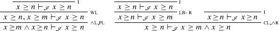
The constant calculus $\vdash _{\mathscr {C}}$ in Fig. 5 is similar to the sign calculus because both logics can only derive $\mathsf {ff}_x$ for each variable. The interval calculus $\vdash _{\mathscr {I}}$ in Fig. 6 contains rules for modifying upper and lower bounds on a variable. Specifically, the order on the integers dictates that one can weaken an upper bound $x \le m$ to $x \le n$ if m is smaller than n and a dual rule applies to lower bounds. It also contains a rule for deriving $\mathsf {ff}_x$ from inconsistent lower and upper bounds.

Example 6

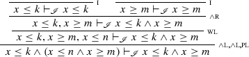
An abstract interpreter computing intervals on variable values will manipulate formulae over multiple variables. Suppose the abstract interpreter has derived the bounds $x \in [7,5], y \in [-\infty , 0]$ for some location in a program. We have deliberately written [7, 5], which would correspond to an empty interval, meaning that there is no feasible value for x and consequently, that the program location for which this bound was derived is unreachable. The conversion of [7, 5] to the empty interval is a calculation an abstract interpreter performs.

Logically, the bounds on x and y can be written as the sequence of predicates $y \le 0, x \le 5 \wedge x \ge 7$. The interval proof calculus allows us to derive the sequent ${y \le 0, x \le 5 \wedge x \ge 7 \vdash _{\mathscr {I}} \mathsf {ff}_x \wedge y \le 0}$ showing that the bound is infeasible and the inconsistency arises from x.

4.2 Soundness of the Proof Systems

Theorem 3 summarizes the soundness results we present, though, we prove the soundness of each calculus separately in Lemmas 3 to 6.

Theorem 3

The proof calculi $\vdash _{\mathscr {S}}$, $\vdash _{\mathscr {C}}$, and $\vdash _{\mathscr {I}}$ are sound.

We begin with the soundness of $\vdash _{\textsc {core}}$, which underlies all our calculi.

Lemma 3

The core proof calculus $\vdash _{{\textsc {core}}}$ is sound.

Proof

We have to show that for every derivable sequent $\Gamma \vdash \varphi$, a structure $\sigma$ that satisfies every formula in $\Gamma$, the structure also satisfies $\varphi$. The proof is by induction on the structure of a derivation.

(Base Case) The base cases are rules with no premise. The introduction (i) and truth ($\mathsf {tt}\textsc {r}$) rules are trivially sound. The false rule is sound because $\mathsf {ff}_x$ has no models.

(Induction Step)  The induction hypothesis is that a sequent derived using the core calculus is sound. For the induction step, we have to show that a sequent obtained by applying rules in the core calculus to a soundly derived sequent is also sound. The weakening rule is sound because if $\bigwedge \Gamma$ implies $\psi$, then $\bigwedge \Gamma \wedge \varphi$ also implies $\psi$ for the standard semantics of conjunction. The left and right conjunction rules are sound for the same reason. The contraction rule is sound because conjunction is idempotent and the permutation rule is sound because conjunction is commutative. $\square$

The soundness proofs for the other proof calculi are extensions of this lemma.

Lemma 4

The sign proof calculus $\vdash _{\mathscr {S}}$ is sound.

Proof

The proof extends the induction argument used for the soundness of the core calculus. Additional conditions for the base case are the rules $\mathsf {ff}\textsc {r}_1$, $\mathsf {ff}\textsc {r}_2$ and $\mathsf {ff}\textsc {r}_3$, which are sound because their premises are unsatisfiable. The induction hypothesis and inductive step are unmodified so the sign calculus is sound. $\square$

Lemma 5

The constant proof calculus $\vdash _{\mathscr {C}}$ is sound.

Proof

The proof extends the induction arguments used for the core calculus. An additional condition for the base case is the rule $\mathsf {ff}\textsc {r}_4$, which is sound because its premise is unsatisfiable. The induction hypothesis and inductive step are unmodified so the constant calculus is sound. $\square$

Lemma 6

The interval proof calculus $\vdash _{\mathscr {I}}$ is sound.

Proof

The proof requires extensions to the base case and induction step of the induction arguments used for proving the soundness of the core calculus. An additional condition for the base case is the rule $\mathsf {ff}\textsc {r}_5$, which is sound because the premise is unsatisfiable. The rules ub-l, lb-l for strengthening bounds on the left, and the rules ub-r, lb-r for weakening bounds on the right are sound due to the order on the integers so the interval calculus is sound.$\square$

5 Characterizing Lattices with First-Order Theories

We now apply the Lindenbaum–Tarski construction to generate a lattice from each logical language and then prove that the generated lattice is isomorphic to a lattice studied in program analysis.

5.1 The Lindenbaum-Tarski Construction and Logical Characterization

Tarski generalized a construction due to Lindenbaum to generate Boolean algebras from propositional calculus [34]. This construction has since be generalized to construct what is called the Lindenbaum–Tarski algebra of a logic. The essence of the construction is to quotient formulae in a logical language with respect to interderivability in that language. These equivalence classes form the carrier set of an algebra whose meet and join operations are defined by lifting conjunction and disjunction to equivalence classes. Derivability between formulae in equivalence classes defines a partial order on equivalence classes. The original construction has been extended to non-classical and first-order logics. We use a generalization of this construction to formulae with free variables due to [32], sometimes called the Rasiowa-Sirkoski construction of a Lindenbaum–Tarski algebra. In the definition below, we write $[\varphi ]_\mathscr {L}$ for the equivalence class of $\varphi$ with respect to $\equiv _\mathscr {L}$.

Definition 1

Let $(\mathscr {L}, \vdash _\mathscr {L})$ be a logical language and $\equiv _\mathscr {L}$ be an equivalence relation on formulae. A logic $(\mathscr {L}, \vdash _\mathscr {L})$ that is closed under conjunction generates the Lindenbaum–Tarski algebra ${ Alg }(\mathscr {L}, \vdash _\mathscr {L}) = ({\mathscr {L}}/{\equiv _\mathscr {L}}, \preccurlyeq _\mathscr {L}, \curlywedge _\mathscr {L})$ in which the relation $\preccurlyeq _\mathscr {L}$ and operator $\curlywedge _\mathscr {L}$ are defined on equivalence classes as shown below.

$$\begin{aligned} \varphi \equiv _\mathscr {L}\psi&\text { if } \varphi \vdash _\mathscr {L}\psi \text { and } \psi \vdash _\mathscr {L}\varphi .\\ [\varphi ]_\mathscr {L}\preccurlyeq _\mathscr {L}[\psi ]_\mathscr {L}&\text { if } \theta _1 \vdash _\mathscr {L}\theta _2 \text { for some } \theta _1\in [\varphi ]_\mathscr {L}, \text { and } \theta _2\in [\psi ]_\mathscr {L}.\\ [\varphi ]_\mathscr {L}\curlywedge _\mathscr {L}[\psi ]_\mathscr {L}&\,\hat{=}\,[\theta _1 \wedge \theta _2]_\mathscr {L}\text { where } \theta _1 \in [\varphi ]_\mathscr {L}, \text { and } \theta _2 \in [\psi ]_\mathscr {L}. \end{aligned}$$

The literature contains characterizations of Lindenbaum–Tarski algebras for various propositional and first-order logics. The classical propositional calculus provides an instructive example of the difference between what we study and what exists. The set of Boolean formulae over n propositional variables is countably infinite. The Lindenbaum–Tarski algebra over these formulae will contain $2^{2^n}$ elements, and is isomorphic to the free Boolean algebra over n generators. A Boolean algebras with $2^{n}$ elements for odd values of n will not be generated by this construction if one only uses the standard complete deductive systems for propositional calculus. The non-free Boolean algebras are Lindenbaum–Tarski algebras of propositional theories, meaning that they require additional axioms.

Example 7

The Lindenbaum–Tarski algebra of a propositional logic with one variable has the elements $\left\{ \mathsf {ff}, p, \lnot p, \mathsf {tt}\right\}$. A propositional logic with two variables generates a lattice with 16 elements. The four, least, non-bottom elements (atoms) are $\left\{ p \wedge q, p \wedge \lnot q, \lnot p \wedge q, \lnot p \wedge \lnot q\right\}$ and the other elements are equivalent to disjunctions of these elements. The lattice $\mathop {\mathcal {P}(\left\{ a,b,c\right\} )}$ has eight elements and is not isomorphic to the Lindenbaum–Tarski algebra of either of these two logics. One way to generate the eight element Boolean algebra using the Lindenbaum–Tarski construction, is to add the axiom $p \wedge q$. Alternative axioms are $p \wedge \lnot q$, $\lnot p \wedge q$ and $\lnot p \wedge \lnot q$.

We show how lattices in abstract interpretation are Lindenbaum–Tarski algebras of first-order theories. Ex. 7 illustrates that different theories generate isomorphic algebras. A characterization of a lattice-based abstraction, defined below, consists of a structural condition and a semantic condition. The structural condition uses a proof system to generate the lattice, and the semantic condition uses the concretization function to express that the logic and the abstraction have the same semantics. There may be multiple isomorphisms h between the Lindenbaum–Tarski algebra and a lattice, intuitively corresponding to different axiomatizations. Only some isomorphisms will satisfy the second condition and capture the semantics of the abstraction.

Definition 2

Let $(A, \sqsubseteq )$ be an abstraction of $(\mathop {\mathcal {P}( Struct )}, \subseteq )$ with concretization function $\gamma : A \rightarrow \mathop {\mathcal {P}( Struct )}$. A logical language $(\mathscr {L}, \vdash _\mathscr {L}, \models _\mathscr {L})$ characterizes $(A, \sqsubseteq )$, if the following conditions hold.

• 1. There exists an isomorphism $h: { Alg }(\mathscr {L}, \vdash _\mathscr {L}, \models _\mathscr {L}) \rightarrow A$ between the Lindenbaum–Tarski algebra of $\mathscr {L}$ and A.

• 2. An element a in A concretizes to the same set of structures as the formula it represents: $mod (\varphi ) = \gamma (h([\varphi ]_\mathscr {L}))$.

We now study the Lindenbaum–Tarski algebras of logical languages corresponding to the sign, constants and interval languages. To avoid cumbersome distinctions between an equivalence class and its representatives, we use the following lemma that allows us to work directly with the syntactic representation of an equivalence class.

Lemma 7

Let $\varphi$ and $\psi$ be two formulae. Then, $[\varphi ] and [\psi ]$ are the same equivalence class if and only if $\varphi \vdash \psi$ and $\psi \vdash \varphi$.

Proof

($\Rightarrow$) Since $[\varphi ]$ and $[\psi ]$ are the same equivalence class there is a formula $\theta$ in $[\varphi ]$ such that $\theta \vdash \varphi$, $\varphi \vdash \theta$, $\theta \vdash \psi$ and $\psi \vdash \theta$. We can now prove $\varphi \vdash \psi$ and $\psi \vdash \varphi$:

$\square$

5.2 Characterization of the Sign Proof Calculus

The lattice of signs $( Sign , \sqsubseteq )$ is depicted in Fig. 3. It consists of five elements $Sign = \left\{ \bot , \mathsf {Neg}, \mathsf {Zero}, \mathsf {Pos}, \top \right\}$ with $\bot$ and $\top$ as the least and greatest elements in the order $\sqsubseteq$, and with the elements in $\left\{ \mathsf {Neg}, \mathsf {Zero}, \mathsf {Pos}\right\}$ being pairwise incomparable. The concretization function $\gamma _ Sign : Sign \rightarrow \mathop {\mathcal {P}(\mathbb {Z})}$ is defined below. For all the lattices we consider, the concretization of $\bot$ is $\emptyset$ and of $\top$ is $\mathbb {Z}$, so we skip these elements.

$$\begin{aligned} \gamma _ Sign (\mathsf {Neg})&= \left\{ n ~|~n < 0\right\}&\gamma _ Sign (\mathsf {Zero})&= \left\{ n ~|~n = 0\right\}&\gamma _ Sign (\mathsf {Pos})&= \left\{ n ~|~n > 0\right\} \end{aligned}$$

The lattice of sign environments $( Vars \rightarrow Sign , \sqsubseteq )$ is the pointwise lift of $Sign$ to a set of functions. We use the same notation for the order and operations and their pointwise lifts. We first prove the special case of isomorphism between the sign logic $\mathscr {S}$ with a single variable and the lattice $\left\{ x\right\} \rightarrow Sign$. Since the lattice $\left\{ x\right\} \rightarrow Sign$ is isomorphic to $Sign$, we do not distinguish between the two. The concretization of a sign environment is defined below.

$$\begin{aligned} \gamma _ Sign&( Vars \rightarrow Sign ) \rightarrow \mathop {\mathcal {P}( Struct )}&\gamma _ Sign (\varepsilon )&= \left\{ \sigma ~|~\sigma (x) \in \gamma _ Sign (\varepsilon (x))\right\} \end{aligned}$$

An environment $\varepsilon$ concretizes to the set of structures that respect the signs of the variables in $\varepsilon$.

Lemma 8

The Lindenbaum–Tarski algebra of the sign logic $\mathscr {S}$ with a single variable has exactly five equivalence classes $\left\{ [\mathsf {ff}_x]_{\mathscr {S}}, [x < 0]_{\mathscr {S}}, [x = 0]_{\mathscr {S}}, [x > 0]_{\mathscr {S}}, [\mathsf {tt}]_{\mathscr {S}} \right\}$.

Proof

We proceed by induction on formula structure and abbreviate $[\varphi ]_{\mathscr {S}}$ to $[\varphi ]$.

 (Base Case) The constants $\mathsf {ff}_x$ and $\mathsf {tt}$, and the atomic formulae $x < 0$, $x = 0$ and $x > 0$ are each in one of these equivalence classes by the introduction rule.

 (Induction Step) The induction hypothesis is that every formula of $\mathscr {S}$ belongs to one of these equivalence classes. For the induction step, consider a formula $\varphi \wedge \psi$, where $[\varphi ]$ and $[\psi ]$ are among the equivalence classes above. We consider four cases for these two equivalence classes.

• 1. The two formulae are in the same equivalence class. By Lemma 7, we have the two sequents $\varphi \vdash _{\mathscr {S}} \psi$ and $\psi \vdash _{\mathscr {S}} \varphi$. The derivations below show that $\varphi \wedge \psi \vdash _{\mathscr {S}} \psi$ and $\psi \vdash _{\mathscr {S}} \varphi \wedge \psi$, so that $[\varphi \wedge \psi ]$ is the same equivalence class as $[\varphi ]$.

  

• 2. The two formulae are in distinct equivalence classes and $[\varphi ]$ is $[\mathsf {ff}_x]$. In this case, $[\varphi \wedge \psi ]$ is also $[\mathsf {ff}_x]$. We prove $\varphi \wedge \psi \vdash _{\mathscr {S}} \mathsf {ff}_x$ and $\mathsf {ff}_x \vdash _{\mathscr {S}} \varphi \wedge \psi$ knowing that $\varphi \vdash _{\mathscr {S}} \mathsf {ff}_x$ and $\mathsf {ff}_x \vdash _{\mathscr {S}} \varphi$. The case for $[\psi ]$ being $[\mathsf {ff}_x]$ is identical.

  

• 3. The two equivalence classes are distinct and $[\varphi ]$ is $[\mathsf {tt}]$. In this case, $[\varphi \wedge \psi ]$ is $[\psi ]$. It suffices to derive $\varphi \wedge \psi \vdash _{\mathscr {S}} \psi$ and $\psi \vdash _{\mathscr {S}} \varphi \wedge \psi$ given $\varphi \vdash _{\mathscr {S}} \mathsf {tt}$ and $\mathsf {tt}\vdash _{\mathscr {S}} \varphi$.

  

  The case for $[\psi ]$ being $[\mathsf {tt}]$ is identical.

• 4. The final case is when $[\varphi ]$ and $[\psi ]$ are distinct and neither of them is the equivalence class of $\mathsf {ff}_x$ or of $\mathsf {tt}$. In this case, we show that $[\varphi \wedge \psi ]$ is $[\mathsf {ff}_x]$ We show that $\varphi \wedge \psi \vdash _{\mathscr {S}} \mathsf {ff}_x$ and $\mathsf {ff}_x \vdash _{\mathscr {S}} \varphi \wedge \psi$ are derivable for all distinct, non-constant, atomic formulae $\varphi$ and $\psi$. By Lemma 7, the induction hypothesis and the assumption that the equivalence classes are not those for logical constants, there are only three cases to consider.

  

The proof so far shows that there are at most five equivalence classes. It does not show that these equivalence classes are distinct, e.g., that there is no way to derive $x > 0$ from $x = 0$ in $\vdash _\mathscr {S}$. The formulae $\left\{ x < 0, x = 0, x > 0\right\}$ do not semantically entail each other, do not entail $\mathsf {ff}_x$ and are not entailed by $\mathsf {tt}$. By the soundness of the sign calculus, it follows that distinct formulae in $Sign$ are pairwise not inter-derivable. $\square$

Lemma 9

The sign logic with a single variable characterizes the abstraction $Sign$.

Proof

Define the function $h : {\mathscr {S}}/{\equiv _{\mathscr {S}}} \rightarrow Sign$ as the witness for the isomorphism.

From Lemma 8, h is a bijection. We show that h is an order isomorphism: $[\varphi ] \preccurlyeq _{\mathscr {S}} [\psi ]$ if and only if $h([\varphi ]) \sqsubseteq h([\psi ])$. We should consider different cases. In the following, for brevity, we write $\preccurlyeq$ for $\preccurlyeq _{\mathscr {S}}$.

• $[\varphi ] \preccurlyeq [\mathsf {tt}] \Leftrightarrow h([\varphi ]) \sqsubseteq h([\mathsf {tt}])$. The implication holds because $h([\mathsf {tt}])$ is $\top$ in the lattice. For the converse we apply the rule for true.

  

• $[\mathsf {ff}_x] \preccurlyeq [\varphi ] \Leftrightarrow h([\mathsf {ff}_x]) \sqsubseteq h([\varphi ])$. The implication holds because $h([\mathsf {ff}_x])$ is $\bot$. The converse holds because of the rule for false.

  

• For all other cases, observe that if $[\varphi ]$ and $[\psi ]$ are incomparable, then so are $h([\varphi ])$ and $h([\psi ])$. Conversely if a is not comparable to b in $Sign$, then, the inverse maps $h^{-1}(a)$ and $h^{-1}(b)$ map to elements that do not entail each other and by soundness of $\vdash _{\mathscr {S}}$, these elements cannot be in the same equivalence class.

It remains to show that h distributes over meets. In the following, for brevity, we write $\curlywedge$ for $\curlywedge _{\mathscr {S}}$. We should consider all possible cases. For example:

• $h([x< 0] \curlywedge [x = 0]) = h([x < 0]) \sqcap h([x = 0])$. We have $h([x< 0] \curlywedge [x = 0]) = h([x< 0 \wedge x = 0]) = h([\mathsf {ff}_x]) = \bot = \mathsf {Neg}\sqcap \mathsf {Zero}= h([x < 0]) \sqcap h([x = 0])$.

The proof is similar for all cases where the meet is bottom. Otherwise, the meet is either of the form $a \curlywedge b$ with either a and b being the same, or one of them being the top element. Verification of these cases is routine.

To complete the proof, we have to show that $\mathscr {S}$ and $Sign$ have the same semantics. By Lemma 4, $\vdash _{\mathscr {S}}$ is sound, so if $[\varphi ]$ and $[\psi ]$ are the same equivalence class, then $mod (\varphi ) = mod (\psi )$. By Lemma 8, we only have to consider one formula in each of the five equivalence classes. Consider $x > 0$.

• We have that $\gamma _ Sign (h(x> 0)) = \gamma _ Sign (\mathsf {Pos}) = \left\{ x\right\} \rightarrow \left\{ n ~|~n > 0\right\}$. Note that we distinguish between $\left\{ x\right\} \rightarrow Sign$ and $Sign$ here because we need to concretize structures. Since $mod (x> 0) = \left\{ (x{:}n) ~|~n > 0\right\}$, the semantic condition follows.

The condition can similarly be verified for the other equivalence classes. $\square$

The chosen isomorphism h is crucial for the semantic condition to hold. Consider the function g that maps $[x < 0]$ to $\mathsf {Pos}$ and $[x > 0]$ to $\mathsf {Neg}$ and otherwise agrees with h. Note that g is an isomorphism but will not satisfy the semantic condition. We show that the sign logic with multiple variables characterizes sign environments.

Lemma 10

In the sign logic $\mathscr {S}$ over a finite set of variables $Vars$, every formula $\varphi$ is inter-derivable with a formula of the form $\bigwedge _{x \in V} \psi (x)$, for some $V \subseteq Vars$.

Proof

The proof is by induction on the number of variables and the structure of $\mathscr {S}$-formulae. The base case is a logic with one variable, which follows from Lemma 8. The induction hypothesis is that the lemma holds for $n \ge 1$ variables. For the induction step, we need to show that the lemma holds for a formula $\varphi$ with $n+1$ variables. First note that $\varphi$ must be of the form $\varphi _1 \wedge \varphi _2$, where at most n variables occur in $\varphi _1$ and $\varphi _2$. This is because the only way to introduce variables is by conjunction with an atomic predicate, the only way to compose formulae is by conjunction and because formulae are finite in length. By the induction hypothesis, $\varphi _1$ and $\varphi _2$ are inter-derivable with formulae of the form $\bigwedge _{x \in V_1} \psi _1(x)$ and $\bigwedge _{x \in V_2} \psi _2(x)$, respectively. Thus, $\varphi _1 \wedge \varphi _2$ is inter-derivable with a formula of the form

$$\begin{aligned} \left( \bigwedge _{x \in V_1 \setminus V_2} \psi _1(x) \right) \wedge \left( \bigwedge _{x \in V_1 \cap V_2} \psi _1(x) \wedge \psi _2(x) \right) \wedge \left( \bigwedge _{x \in V_2 \setminus V_1} \psi _2(x) \right) \end{aligned}$$

which is of the form in the lemma. $\square$

Lemma 11

The logic $\mathscr {S}$ over a finite set of variables $Vars$ characterizes the lattice of sign environments $( Vars \rightarrow Sign , \sqsubseteq )$.

Proof

Let h be the isomorphism from $\mathscr {S}$ to $Sign$ for the one variable case from Lemma 9. In the following, we write $var (\varphi )$ for the set of variables in a formula. Define the candidate isomorphism $g : {\mathscr {S}}/{\equiv _{\mathscr {S}}} \rightarrow ( Vars \rightarrow Sign )$ as follows:

$$\begin{aligned} g([\varphi ])(x) \,\hat{=}\,{\left\{ \begin{array}{ll} h([\psi (x)]) &{} x \in var (\varphi ) \\ \top &{} x \notin var (\varphi ) \end{array}\right. } \end{aligned}$$

Note that $Vars \rightarrow Sign$ is isomorphic to the product lattice $Sign ^{| Vars |}$. We have to show that there are as many equivalence classes as elements in the product lattice. It follows from Lemma 10 that every equivalence class can be written as the conjunction $\bigwedge _{x \in var (\varphi )} \psi (x)$, where every formula $\psi (x)$ belongs to one equivalence class of $\mathscr {S}$ over one variable. Thus, by Lemma 8 and the rule $\wedge \textsc {r}$, we can combine a derivation of each individual formula to obtain a derivation of the entire conjunction. It follows that there are at least as many equivalence classes as elements in the product. To show that there are at most as many equivalence classes, we observe that every formula of the form $\bigwedge _{x \in V} \psi (x)$, for some $V \subseteq Vars$, is inter-derivable with a formula of the form $\bigwedge _{x \in V} \psi (x) \wedge \bigwedge _{x \in Vars \setminus V} \mathsf {tt}$. Thus, every formula $\varphi$ derivable from a formula of the form $\bigwedge _{x \in V} \psi (x)$, for some $V \subseteq Vars$, is of the form $\bigwedge _{x \in V} \psi (x) \wedge \bigwedge _{x \in Vars \setminus V} \mathsf {tt}$. By lifting the proof of Lemma 9 component-wise, we can conclude that g is an isomorphism.

To verify the semantic condition. consider $\varepsilon$ in $mod (\varphi )$. By Lemma 10, $\varphi$ is equivalent to some $\bigwedge _{x \in var (\varphi )} \psi (x)$, so $\varepsilon (x)$ is a value satsifying $\psi (x)$. By Lemma 9, $\varepsilon (x)$ is also in $\gamma _ Sign (h([\psi (x)]))$. It follows from the definition of g that $\varepsilon (x)$ is in $\gamma _ Sign (g([\varphi ])(x))$ for each x. From the definition of concretization for sign environments, it follows that $\varepsilon$ is in $\gamma _ Sign (g([\varphi ]))$. $\square$

Example 8

This example shows that the proof system of the sign calculus is incomplete and this incompleteness is fundamental to characterizing sign environments. Consider the lattice $Sign$ and the sign environments $\left\{ x, y\right\} \rightarrow Sign$. Three distinct sign environments and their logical representations are shown below.

$$\begin{aligned} \varepsilon _1&= \left\{ x \mapsto \mathsf {Pos}, y \mapsto \bot \right\}&\varepsilon _2&= \left\{ x \mapsto \bot , y \mapsto \mathsf {Neg}\right\}&\varepsilon _3&= \left\{ x \mapsto \bot , y \mapsto \bot \right\} \\ h^{-1}(\varepsilon _1)&= [x > 0 \wedge \mathsf {ff}_y]&h^{-1}(\varepsilon _2)&= [\mathsf {ff}_x \wedge y < 0]&h^{-1}(\varepsilon _3)&= [\mathsf {ff}_x \wedge \mathsf {ff}_y] \end{aligned}$$

Observe that none of the formulae are satisfiable. In order for the the Lindenbaum–Tarski algebra to be isomorphic to the lattice of sign environments, we need that the formulae are not inter-derivable. That is, the proof system must be incomplete.

5.3 Characterization of the Constant Proof Calculus

The lattice of integer constants $( Const , \sqsubseteq )$ is depicted in Fig. 5. It consists of the elements $Const = \mathbb {Z}\cup \left\{ \bot , \top \right\}$, with $\bot$ and $\top$ as the least and greatest elements, and with all other elements being incomparable. The concretization $\gamma _ Const : Const \rightarrow \mathop {\mathcal {P}(\mathbb {Z})}$ maps n to $\left\{ n\right\}$. The concretization for constant environments $Vars \rightarrow Const$ is defined in a similar manner to the concretization for sign environments. We prove the characterization for the one-variable case and then generalize to more variables.

Lemma 12

The set of equivalence classes of the Lindenbaum–Tarski algebra of the constant logic $\mathscr {C}$ with a single variable is $\left\{ [\mathsf {ff}_x]_{\mathscr {C}}\right\} \cup \left\{ [x = k]_{\mathscr {C}}~|~k \in \mathbb {Z}\right\} \cup \left\{ [\mathsf {tt}]_{\mathscr {C}}\right\}$.

Proof

The proof is similar to the proof of Lemma 8. We reason by induction on the structure of the formulae of $\mathscr {C}$. We abbreviate $[\varphi ]_{\mathscr {C}}$ to $[\varphi ]$.

(Base Case) The constants $\mathsf {ff}_x$ and $\mathsf {tt}$, and the atomic formulae $x = k$ are, by the introduction rule of the core calculus, in one of these equivalence classes.

(Induction Step) The induction hypothesis is that every formula of $\mathscr {C}$ belongs to one of these equivalence classes. For the induction step, consider a formula $\varphi \wedge \psi$. When $\varphi$ and $\psi$ are in the same equivalence class, as in Lemma 8 we have $\varphi \wedge \psi \vdash _{\mathscr {C}} \psi$ and $\psi \vdash _{\mathscr {C}} \varphi \wedge \psi$, so that $[\varphi \wedge \psi ]$ is the same class as $[\varphi ]$. If the two equivalence classes are distinct, we have to consider if they are comparable or incomparable. Comparisons are only possible if one of the equivalence classes is $[\mathsf {ff}_x]$ or is $[\mathsf {tt}]$. If either $[\varphi ]$ or $[\psi ]$ is $[\mathsf {ff}_x]$, as in Lemma 8 we have $\varphi \wedge \psi \vdash _{\mathscr {C}} \mathsf {ff}_x$ and $\mathsf {ff}_x \vdash _{\mathscr {C}} \varphi \wedge \psi$, so $[\varphi \wedge \psi ]$ is also $[\mathsf {ff}_x]$. If $[\varphi ]$ is $[\mathsf {tt}]$, as in Lemma 8 we have $\varphi \wedge \psi \vdash _{\mathscr {C}} \psi$ and $\psi \vdash _{\mathscr {C}} \varphi \wedge \psi$, so $[\varphi \wedge \psi ]$ is $[\psi ]$. The case for $[\psi ]$ being $[\mathsf {tt}]$ is identical. If $[\varphi ]$ and $[\psi ]$ are distinct and are not the equivalence classes of $\mathsf {ff}_x$ and $\mathsf {tt}$, we show that $[\varphi \wedge \psi ]$ is $[\mathsf {ff}_x]$. We show that $\varphi \wedge \psi \vdash _{\mathscr {C}} \mathsf {ff}_x$ and $\mathsf {ff}_x \vdash _{\mathscr {C}} \varphi \wedge \psi$ are derivable for all distinct, non-constant, atomic formulae $x = m$ and $x = n$.

The equivalence classes are distinct because the constant calculus is sound. $\square$

Lemma 13

Constant logic with one variable characterizes the lattice of constants.

Proof

Define the function $h : {\mathscr {C}}/{\equiv _{\mathscr {C}}} \rightarrow Const$ as the witness for the isomorphism.

$$\begin{aligned} h([\mathsf {tt}])&~\,\hat{=}\,~\top&h([x = k])&~\,\hat{=}\,~k&h([\mathsf {ff}_x])&~\,\hat{=}\,~\bot \end{aligned}$$

From Lemma 12, h is a bijection. The proof that h is an order isomorphism and distributes over meets is identical to the proof of Lemma 9 and verification of the semantic condition is straightforward. $\square$

The following result now shows that the Lindenbaum–Tarski algebra of the constant logic $\mathscr {C}$ is isomorphic to the pointwise lift $Vars \rightarrow \mathscr {C}$ of $\mathscr {C}$.

Lemma 14

Constant logic over a finite set of variables $Vars$ characterizes the constant environments $( Vars \rightarrow Const , \sqsubseteq )$.

Proof

The proof is identical to the proof of Lemma 11 using the candidate isomorphism $g : {\mathscr {C}}/{\equiv _{\mathscr {C}}} \rightarrow ( Vars \rightarrow Const )$:

$$\begin{aligned} g([\varphi ])(x) \,\hat{=}\,{\left\{ \begin{array}{ll} h([\psi (x)]) &{} x \in var (\varphi ) \\ \top &{} x \notin var (\varphi ) \end{array}\right. } \end{aligned}$$

where h is the isomorphism from the Lindenbaum–Tarski algebra of $\mathscr {C}$ to the lattice $Const$ of constants for the one variable case from Lemma 13. The concretization for constant environments is defined in a similar manner to the concretization for sign environments, hence the verification of the semantic condition is also similar. $\square$

5.4 Characterization of the Interval Proof Calculus

The lattice of integer intervals $( Itv , \sqsubseteq )$ is depicted in Fig. 6. It consists of the set $\left\{ [a,b] ~|~a\le b, a \in \mathbb {Z}\cup \left\{ -\infty \right\} , b \in \mathbb {Z}\cup \left\{ \infty \right\} \right\}$ and a special element $\bot$ denoting the empty interval. The partial order is standard and $[-\infty , \infty ]$ is the top element. The concretization is $\gamma _ Itv ([a,b]) = \left\{ n \in \mathbb {Z}~|~a \le n \le b\right\}$ for non-$\bot$ elements. The lattice of interval environments is $( Vars \rightarrow Itv , \sqsubseteq )$ with the pointwise order. The concretization of an interval environment is defined similarly to concretization for sign environments: $\gamma _ Itv (\varepsilon ) = \left\{ \sigma ~|~\sigma (x) \in \gamma _ Itv (\varepsilon (x))\right\}$. We characterize $Itv$ by the interval logic $\mathscr {I}$ over one variable.

Lemma 15

The set of equivalence classes of the Lindenbaum–Tarski algebra of the interval logic $\mathscr {I}$ with a single variable is $\left\{ [x \le k]_{\mathscr {I}}~|~k \in \mathbb {Z}\right\} \cup \left\{ [x \ge k]_{\mathscr {I}}~|~k \in \mathbb {Z}\right\} \cup \left\{ [x \le n \wedge x \ge m]_{\mathscr {I}}~|~m,n \in \mathbb {Z}, m \le n\right\} \cup \left\{ [\mathsf {ff}_x]_{\mathscr {I}}, [\mathsf {tt}]_{\mathscr {I}}\right\}$.

Proof

The proof is by induction on formula structure. We write $[\varphi ]_{\mathscr {I}}$ for $[\varphi ]$.

 (Base Case) The constants $\mathsf {ff}_x$ and $\mathsf {tt}$, and the atomic formulae $x \ge k$ and $x \le k$ are, by the introduction rule of the core calculus, in one of these equivalence classes.

 (Induction Step)  The induction hypothesis is that every formula of $\mathscr {I}$ belongs to one of these equivalence classes. For the induction step, consider a formula $\varphi \wedge \psi$. When $\varphi$ and $\psi$ are in the same equivalence class, as in Lemma 8 we have $\varphi \wedge \psi \vdash _{\mathscr {I}} \psi$ and $\psi \vdash _{\mathscr {I}} \varphi \wedge \psi$, so that $[\varphi \wedge \psi ]$ is the same class as $[\varphi ]$. If the equivalence classes are distinct, we have to consider the cases where there is either an order between the classes or they are incomparable. If either $[\varphi ]$ or $[\psi ]$ is $[\mathsf {ff}_x]$, as in Lemma 8 we have $\varphi \wedge \psi \vdash _{\mathscr {I}} \mathsf {ff}_x$ and $\mathsf {ff}_x \vdash _{\mathscr {I}} \varphi \wedge \psi$, so $[\varphi \wedge \psi ]$ is also $[\mathsf {ff}_x]$. If $[\varphi ]$ is $[\mathsf {tt}]$, as in Lemma 8 we have $\varphi \wedge \psi \vdash _{\mathscr {I}} \psi$ and $\psi \vdash _{\mathscr {I}} \varphi \wedge \psi$, so $[\varphi \wedge \psi ]$ is $[\psi ]$. The case for $[\psi ]$ being $[\mathsf {tt}]$ is identical. If $[\varphi ]$ and $[\psi ]$ are distinct and are not the equivalence classes of $\mathsf {ff}_x$ and $\mathsf {tt}$, without loss of generality have the following cases:

• 1. If $[\varphi ]$ is $[x \le m]$ and $[\psi ]$ is $[x \le n]$, then, if $m < n$, we have that $[\varphi \wedge \psi ]$ is $[\varphi ]$. We show that $\varphi \wedge \psi \vdash _{\mathscr {I}} \varphi$ and $\varphi \vdash _{\mathscr {I}} \varphi \wedge \psi$ are derivable.

  

  Otherwise, if $n < m$, we have that $[\varphi \wedge \psi ]$ is $[\psi ]$. The proof is similar, requiring an application of the ${\textsc {pl}}$ rule before the ${\textsc {wl}}$ rule.

• 2. If $[\varphi ]$ is $[x \ge m]$ and $[\psi ]$ is $[x \ge n]$, then $[\varphi \wedge \psi ]$ is $[\psi ]$ if $m < n$ and is $[\varphi ]$ if $n < m$. The proof is similar to the previous case but uses the ${\textsc {lb-r}}$ rule instead of ${\textsc {ub-l}}$. The following derivations shows that, if $m < n$, $[\varphi \wedge \psi ]$ is $[\psi ]$.

  

  The derivations showing that, if $n < m$, $[\varphi \wedge \psi ]$ is $[\varphi ]$ are almost identical except that the ${\textsc {pl}}$ rule need not be applied before ${\textsc {wl}}$.

• 3. If $[\varphi ]$ is $[x \le n]$ and $[\psi ]$ is $[x \ge m]$, then, if $m \le n$, by the introduction rule, we have that $[\varphi \wedge \psi ]$ is $[x \le n \wedge x \ge m]$. Otherwise, if $n < m$, we have that $[\varphi \wedge \psi ]$ if $[\mathsf {ff}_x]$. We show that $\varphi \wedge \psi \vdash _{\mathscr {S}} \mathsf {ff}_x$ and $\mathsf {ff}_x \vdash _{\mathscr {S}} \varphi \wedge \psi$ are derivable.

  

• 4. If $[\varphi ]$ is $[x \le k]$ and $[\psi ]$ is $[x \le n \wedge x \ge m]$, then we have three cases.

  (case A) If $m \le n < k$ we have that $[\varphi \wedge \psi ]$ is $[\psi ]$. We show that $\varphi \wedge \psi \vdash _{\mathscr {S}} \psi$ and $\psi \vdash _{\mathscr {S}} \varphi \wedge \psi$ are derivable.

  

  (case B) If $m \le k \le n$ we have that $[\varphi \wedge \psi ]$ is $[x \le k \wedge x \ge m]$. We show that $\varphi \wedge \psi \vdash _{\mathscr {S}} x \le k \wedge x \ge m$ is derivable.

  

  The following derivation shows that $x \le k \wedge x \ge m \vdash _{\mathscr {S}} \varphi \wedge \psi$.

  

  (case C) If $k < m \le n$ we have that $[\varphi \wedge \psi ]$ is $[\mathsf {ff}_x]$. We show that $\varphi \wedge \psi \vdash _{\mathscr {S}} \mathsf {ff}_x$ and $\mathsf {ff}_x \vdash _{\mathscr {S}} \varphi \wedge \psi$ are derivable.

  

• 5. If $[\varphi ]$ is $[x \ge k]$ and $[\psi ]$ is $[x \le n \wedge x \ge m]$, then, we also have three cases.

  (case A) If $k < m \le n$, we have that $[\varphi \wedge \psi ]$ is $[\psi ]$. The proof of the derivation $\varphi \wedge \psi \vdash _{\mathscr {I}} \psi$ is identical to case 4A. The derivation showing that $\psi \vdash _{\mathscr {I}} \varphi \wedge \psi$ requires an application of the ${\textsc {pl}}$ rule also before the ${\textsc {wl}}$ rule.

  (case B) f $m \le k \le n$ we have that $[\varphi \wedge \psi ]$ is $[x \le n \wedge x \ge k]$. The derivation showing that $\varphi \wedge \psi \vdash _{\mathscr {I}} x \le n \wedge x \ge k$ is almost identical to case 4B except for requiring an application of the ${\textsc {pl}}$ rule after the ${\textsc {wl}}$ rule. The derivation showing that $x \le n \wedge x \ge k \vdash _{\mathscr {I}} \varphi \wedge \psi$ requires an an application of the ${\textsc {pl}}$ rule also before the ${\textsc {wl}}$ rule and an application of the ${\textsc {lb-l}}$ instead of the ${\textsc {ub-l}}$ rule.

  (case C) If $m \le n < k$ we have that $[\varphi \wedge \psi ]$ is $[\mathsf {ff}_x]$. The derivations are identical to case 4C except for requiring an application of the ${\textsc {pl}}$ rule after the ${\textsc {wl}}$ rule.

• 6. If $[\varphi ]$ is $[x \le q \wedge x \ge p]$ and $[\psi ]$ is $[x \le n \wedge x \ge m]$, then we have five cases.

  (case A) If $p \le m \le n \le q$, we have that $[\varphi \wedge \psi ]$ is $[\psi ]$. The derivation $\varphi \wedge \psi \vdash _{\mathscr {I}} \psi$ is identical to case 4A. The proof that $\psi \vdash _{\mathscr {I}} \varphi \wedge \psi$ is derivable is given below.

  

  (case B) If $m \le p \le q \le n$, we have that $[\varphi \wedge \psi ]$ is $[\varphi ]$. The derivation $\varphi \wedge \psi \vdash _{\mathscr {I}} \varphi$ only requires an application of $\wedge \textsc {l}$, ${\textsc {wl}}$, and the introduction rule. The derivation $\varphi \vdash _{\mathscr {I}} \varphi \wedge \psi$ is identical to case 6A.

  (case C) If $p \le m \le q \le n$, we have that $[\varphi \wedge \psi ]$ is $[x \le q \wedge x \ge m]$. The derivation showing that $\varphi \wedge \psi \vdash _{\mathscr {I}} x \le q \wedge x \ge m$ is almost identical to case 5B except for requiring an application of $\wedge \textsc {l}$, ${\textsc {wl}}$, and ${\textsc {pl}}$ before $\wedge \textsc {r}$. The derivation showing that $x \le q \wedge x \ge m \vdash _{\mathscr {I}} \varphi \wedge \psi$ is given below.

  

  (case D) If $m \le p \le n \le q$, we have that $[\varphi \wedge \psi ]$ is $[x \le n \wedge x \ge p]$. The derivation showing that $\varphi \wedge \psi \vdash _{\mathscr {I}} x \le q \wedge x \ge m$ is almost identical to case 6C except for requiring the application of ${\textsc {pl}}$ after (and not before) the first application of the ${\textsc {wl}}$ rule and the last application of $\wedge \textsc {l}$. The derivation $x \le n \wedge x \ge p \vdash _{\mathscr {I}} \varphi \wedge \psi$ is identical to case 6C.

  (case E) If $q < m$ or $n < p$ we have that $[\varphi \wedge \psi ]$ is $[\mathsf {ff}_x]$. If $q < m$, the proof is similar to case 4C except for requiring the applications of pl, $\wedge \textsc {l}$, ${\textsc {wl}}$, and again ${\textsc {pl}}$ before applying $\mathsf {ff}\textsc {r}_5$. If $n < p$, the proof is similar case 5C except for requiring the applications of $\wedge \textsc {l}$, ${\textsc {pl}}$ and ${\textsc {wl}}$ before applying $\mathsf {ff}\textsc {r}_5$.

The equivalence classes are distinct because the interval calculus is sound. $\square$

Lemma 16

The interval logic over one variable characterizes $Itv$.

Proof

Define the function $h : {\mathscr {I}}/{\equiv _{\mathscr {I}}} \rightarrow Itv$ as the witness for the isomorphism.

From Lemma 15, h is a bijection. We show that h is an order isomorphism: $[\varphi ] \preccurlyeq _{\mathscr {I}} [\psi ]$ if and only if $h([\varphi ]) \sqsubseteq h([\psi ])$. We have different other cases to consider. In the following, for brevity, we write $\preccurlyeq$ for $\preccurlyeq _{\mathscr {I}}$.

• $[\varphi ] \preccurlyeq [\mathsf {tt}] \Leftrightarrow h([\varphi ]) \sqsubseteq h([\mathsf {tt}])$. The implication holds because $h([\mathsf {tt}]) \,\hat{=}\,\top$. For the converse we apply the rule for true as in Lemma 9.

• $[\mathsf {ff}_x] \preccurlyeq [\varphi ] \Leftrightarrow h([\mathsf {ff}_x]) \sqsubseteq h([\varphi ])$. The implication holds because $h([\mathsf {ff}_x]) \,\hat{=}\,\bot$. The converse holds because of the rule for false as in Lemma 9.

• $[x \le m] \preccurlyeq [x \le n] \Leftrightarrow h([x \le m]) \sqsubseteq h([x \le n])$, for any given $m, n \in \mathbb {Z}$ such that $m \le n$. The implication holds because $h([x \le m]) \,\hat{=}\,[-\infty ,m]$ and $h([x \le n]) \,\hat{=}\,[-\infty ,n]$. The converse holds because of the ${\textsc {ub-l}}$ rule and the introduction rule.

  

• $[x \ge n] \preccurlyeq [x \ge m] \Leftrightarrow h([x \ge n]) \sqsubseteq h([x \ge m])$, for any given $m, n \in \mathbb {Z}$ such that $m \le n$. The implication holds because $h([x \ge n]) \,\hat{=}\,[n,+\infty ]$ and $h([x \ge m]) \,\hat{=}\,[m,+\infty ]$. The converse holds because of the ${\textsc {lb-l}}$ rule and the introduction rule.

• $[x \le n \wedge x \ge m] \preccurlyeq [x \le k] \Leftrightarrow h([x \le n \wedge x \ge m]) \sqsubseteq h([x \le k])$, for any given $k, m, n \in \mathbb {Z}$ such that $m \le n \le k$. The implication holds because $h([x \le n \wedge x \ge m]) \,\hat{=}\,[m,n]$ and $h([x \le k]) \,\hat{=}\,[-\infty ,k]$. The converse is show below.

  

• $[x \le n \wedge x \ge m] \preccurlyeq [x \ge k] \Leftrightarrow h([x \le n \wedge x \ge m]) \sqsubseteq h([x \ge k])$, for any given $k, m, n \in \mathbb {Z}$ such that $k \le m \le n$. The implication holds because $h([x \le n \wedge x \ge m]) \,\hat{=}\,[m,n]$ and $h([x \ge k]) \,\hat{=}\,[k,+\infty ]$. The converse is similar to the previous case except for also requiring ${\textsc {pl}}$ before ${\textsc {wl}}$ and for requiring the ${\textsc {lb-l}}$ rule instead of ${\textsc {ub-l}}$.

• $[x \le n \wedge x \ge m] \preccurlyeq [x \le q \wedge x \ge p] \Leftrightarrow h([x \le n \wedge x \ge m]) \sqsubseteq h([x \le q \wedge x \ge p])$, for any given $m, n, p, q \in \mathbb {Z}$ such that $p \le m \le n \le q$. The implication holds because $h([x \le n \wedge x \ge m]) \,\hat{=}\,[m,n]$ and $h([x \le q \wedge x \ge p]) \,\hat{=}\,[p,q]$. The converse is below.

  

• For all other cases, if $[\varphi ]$ and $[\psi ]$ are incomparable, then so are $h([\varphi ])$ and $h([\psi ])$. Conversely if a is not comparable to b in $Sign$, then, the inverse maps $h^{-1}(a)$ and $h^{-1}(b)$ map to elements that do not entail each other and by soundness of the interval calculus, these elements cannot be in the same equivalence class.

It remains to show that h distributes over meets. In the following, for brevity, we write $\curlywedge$ for $\curlywedge _{\mathscr {I}}$. We should consider all possible cases. For example:

• $h([x \le n \wedge x \ge m] \curlywedge [x \le q \wedge x \ge p]) = h([x \le n \wedge x \ge m]) \sqcap h([x \le q \wedge x \ge p])$ where $p \le m \le q \le n$. We have $h([x \le n \wedge x \ge m] \curlywedge [x \le q \wedge x \ge p]) = h([(x \le n \wedge x \ge m) \wedge (x \le q \wedge x \ge p)]) = h([x \le q \wedge x \ge m]) = [m,q] = [m,n] \sqcap [p,q] = h([x \le n \wedge x \ge m]) \sqcap h([x \le q \wedge x \ge p])$.

The reasoning is analogous for all other cases.

The argument for the semantic condition is similar to that for sign logic. $\square$

It is worth noting the difference in the proofs of the condition and the semantic condition in Lemmas 9, 13 and 16. Reasoning about Lindenbaum–Tarski algebras is specific to and proportional in complexity to the axioms of the theory. The concretization functions for all abstractions are defined similarly, so verifying the semantic condition requires the same reasoning in each case.

Lemma 17

The logic $\mathscr {I}$ over a finite set of variables $Vars$ characterizes the interval environments $( Vars \rightarrow Itv , \sqsubseteq )$.

Proof

The proof is identical to the proof of Lemma 11 using the candidate isomorphism $g : {\mathscr {I}}/{\equiv _{\mathscr {I}}} \rightarrow ( Vars \rightarrow Itv )$:

$$\begin{aligned} g([\varphi ])(x) \,\hat{=}\,{\left\{ \begin{array}{ll} h([\psi (x)]) &{} x \in var (\varphi ) \\ \top &{} x \notin var (\varphi ) \end{array}\right. } \end{aligned}$$

where h is the isomorphism from the Lindenbaum–Tarski algebra of $\mathscr {I}$ to the lattice $Itv$ of intervals for the one variable case from Lemma 16. Verifying the semantic condition is as in Lemma 11.

6 Related Work and Discussion

We discuss our work from a conceptual perspective and from the viewpoint of current theoretical and practical research.

6.1 Related Work

Automata, Logic and Languages. A classic family of results shows that regular expressions, finite automata over finite words, and ws1s all define regular languages. We refer to the survey by [38] for equally classic extensions of those results to infinite words and trees. Our work has applied this perspective to programs by using Büchi’s construction to define the set of executions in a control-flow graph by a formula in ws1s(t). The standard, algorithmic approach to reasoning about regular expressions and ws1s is to compile them to automata. We have shown that abstract interpreters can be viewed as solvers for ws1s(t) formulae, which use a graph structure to represent second-order constraints, but use deductive techniques to reason about first-order constraints. Our encoding differs from the use of set constraints by [2] and second-order Horn clauses by [19] in that models of our formulae are erroneous executions, not invariants.

Algebraic Logic and Stone Duality. The framework of Stone duality relate categories of lattices with operators, posets with relations, and topological spaces [26]. Since the Lindenbaum–Tarski construction generates lattices with operators, Stone duality can be viewed as a way to move between different representations of a theory. [1] extended Stone duality to lambda calculi by characterizing domains in semantics. We believe that logical characterization of strictness analysis by [25] was the first application of Stone duality to abstract interpretation. Both Abramsky and Jensen characterized the structures they studied as Lindenbaum–Tarski algebras of propositional, modal, intuitionistic logics. The lattices we studied are non-distributive and arise as algebras of first-order theories. Moreover, the lattices we studied are complete, so the topological machinery of Stone duality is not required to obtain a representation of the theories involved.

The approach we used is influenced by [33], who first articulated the ideas in Table 1 that the partial order in a lattice can be viewed as the proof theory of a logic, and that the concretization function defines the model-theoretic semantics of the logic. Schmidt formalized this view and studied the relationship between soundness and completeness in a logic and the corresponding notions in abstract interpretation. In our work, we have identified proof calculi for specific lattices and have identified a new connection between the Lindenbaum–Tarski construction and abstract interpretation.

Abstract Interpretation and Satisfiability. A driving force behind much current research is the discovery of novel combinations of automated deduction and abstract interpretation. The dissertations of  [22] and [35] and Dagstuhl seminar notes of  [28] provide a summary of this research. This paper contributes to this programme by providing a logical characterizations of an instance of abstract interpretation.

The general theme of work lifting the internals of sat and smt solvers to abstract domains has been to provide a property-guided, on-demand refinement of abstract interpretation-based analysis. dpll(t) and cdcl have been lifted to implement property-guided, path-sensitive analyses [16, 23]. Stålmarck’s method has been used to refine abstract transformers [36], interpolants have been used to refine widening operators [20] and unification has been used to obtain complete reasoning about restricted families of programs [39]. The Nelson-Oppen procedure, though less general than reduced product [10, 11], works as an algorithmic domain combinator [21].

Conversely, abstract interpretation has been incorporated in smt and constraint solvers to improve theory propagation [31, 40], to use joins for space-efficient representation [4], and to use widening for generalization [29]. Algorithms based on abstract interpretation have been used to implement alternatives to dpll(t)  [5, 37] and to improve sat encodings [6].

Theoretical work combining automated deduction and abstract interpretation has attempted to give abstract interpretation formulations of smt solvers [11, 17, 36]. While it is natural to model the algebraic content of a solver in an order-theoretic way, it is cumbersome to model combinatorial aspects such as decision heuristics and precise details of conflict analysis. We also believe that the work discussed above uses a mathematical framework that is atypical for formalizing solver algorithms. For these reasons, we have attempted a logical description of abstract interpretation.

6.2 Applications and Extensions

We briefly discuss potential applications of this work. The practical motivation for this work was to lift the clause learning capabilities of sat and smt solvers to abstract interpreters. We have used the theoretical framework of § 2 and § 3 to develop an abstract interpretation for termination analysis that combines propagation and learning [15].

Another application is to determine the correctness of an analyzer, which is crucial since abstract interpreters are often used to reason about safety-critical software. We refer to [8] for a survey of work on constructing analyzers with proof assistants and [27] for a recent highlight of this research programme. Developing an analyzer in a proof assistant incurs performance penalties, requires significant development time and does not provide confidence in the correctness of existing, deployed analyzers. An alternative, inspired by proof-producing sat and smt solvers, is to have the analyzer generate a proof certificate. Since most abstract interpreters have a modular architecture and rely on an abstract domain library, it would be sufficient to equip such a library with the ability to generate proof certificates. Our work is a step towards this goal; we have shown how to obtain proofs for reasoning performed within a lattice. In order to apply to analyzers used in practice, our proof-theoretic characterization has to extend to transformers and we need such characterizations for analyzers used in practice.

A third motivation is to bring tools and techniques from logic and automated deduction to abstract interpreters. Given the logical characterizations in this paper, one can study cut elimination, proof size, interpolation, and other properties of an abstract interpreter. Without this work, it would not even be clear that these notions apply to an abstract domain.

7 Conclusion

This work advances the logical understanding of the internals of abstract interpreters. Our results make precise widespread folk intuition that abstract domains correspond to monadic logics that are closed under conjunction. In undertaking an explicit study, we have also highlighted the non-standard treatment of false, the limited structure of the sequents involved and the absence of terms. Though our results are unsurprising, we believe such a study contributes in novel ways to the broader research programme of studying logic and abstract interpretation.

The next steps are a characterization of transformers as modalities. We believe this step will bring new challenges and insights as first-order modal theories have received little attention in the literature. We are also not aware of a logical account of widening and narrowing operators and believe that an advance there would need to connect with approaches for inductive generalization.

In summary, we believe that our work leads to several theoretical and practical questions that can be studied from the viewpoint of automated deduction or abstract interpretation. We have begun these investigations and hope that this exposition enables the automated deduction community to participate in the same.

References

Abramsky, S.: Domain theory and the logic of observable properties. PhD thesis, University of London (1987)
Aiken, A.: Introduction to set constraint-based program analysis. Sci. Comput. Program. 35, 79–111 (1999)
Bjørner, N., de Moura, L.: Applications of SMT solvers to program verification. In: Notes for the Summer School on Formal Techniques (2014)
Bjørner, N., Duterte, B., de Moura, L.: Accelerating lemma learning using joins – DPLL(\(\sqcup \)). In: Proceedings of Logic for Programming, Artificial Intelligence and Reasoning (2008)
Brain, M., D’silva, V., Griggio, A., Haller, L., Kroening, D.: Deciding floating-point logic with abstract conflict driven clause learning. Form. Methods Syst. Des. 45(2), 213–245 (2014)
Brain, M., Hadarean, L., Kroening, D., Martins, R., Automatic generation of propagation complete SAT encodings. In: Proceedings of Verification, Model Checking and Abstract Interpretation, Springer, pp. 536–556. (2016)
Büchi, J. R.: On a decision method in restricted second order arithmetic. In: Logic, Methodology and Philosophy of Science, Stanford Univ. Press, pp 1–11 (1960)
Cachera, D., Pichardie, D., Comparing techniques for certified static analysis. In: The NASA Formal Methods Symposium (NFM), NASA Ames Research Center, pp. 111–115. (2009)
Cousot, P., Cousot, R.: Abstract interpretation: a unified lattice model for static analysis of programs by construction or approximation of fixpoints. In: Proceedings of Principles of Programming Languages, ACM Press, pp. 238–252. (1977)
Cousot, P., Cousot, R.: Systematic design of program analysis frameworks. In: Proceedings of Principles of Programming Languages, ACM Press, pp. 269–282. (1979)
Cousot, P., Cousot, R., Mauborgne, L.: Theories, solvers and static analysis by abstract interpretation. J. ACM 59(6), 31:1–31:56 (2013)
Dalla Preda, M., Giacobazzi, R., Lakhotia, A., Mastroeni, I.: Abstract symbolic automata: Mixed syntactic/semantic similarity analysis of executables. In: Proceedings of Principles of Programming Languages, ACM Press, pp. 329–341. (2015)
D’antoni, L.: Extended symbolic finite automata and transducers. Form. Methods Syst. Des. 47(1), 93–119 (2015)
D’Silva, V., Urban, C.: Abstract interpretation as automated deduction. In: Proceedings of Automated Deduction, pp. 450–464. (2015a)
D’Silva, V., Urban, C.: Conflict-driven conditional termination. In: Proceedings of Computer Aided Verification, pp. 471–286. (2015b)
D’Silva, V., Haller, L., Kroening, D.: Abstract conflict driven learning. In: Proceedings of Principles of Programming Languages, ACM Press, pp. 143–154. (2013)
D’Silva, V., Haller, L., Kroening, D.: Abstract satisfaction. In: Proceedings of Principles of Programming Languages, ACM Press, pp. 139–150. (2014)
van den Elsen, S.: Weak monadic second-order theory of one successor. Seminar: Decision Procedures, (2012) http://www.mpi-sws.org/~piskac/teaching/decpro-ws12/slides/WS1S.pdf
Grebenshchikov, S., Lopes, N. P., Popeea, C., Rybalchenko, A.: Synthesizing software verifiers from proof rules. In: Proceedings of Programming Language Design and Implementation, ACM Press, pp. 405–416. (2012)
Gulavani, B. S., Chakraborty, S., Nori, A. V., Rajamani, S. K.: Automatically refining abstract interpretations. In: Proceedings of Tools and Algorithms for the Construction and Analysis of Systems, Springer, LNCS, vol 4963, pp. 443–458. (2008)
Gulwani, S., Tiwari, A.: Combining abstract interpreters. In: Proceedings of Programming Language Design and Implementation, ACM Press, pp. 376–386. (2006)
Haller, L.C.R.: Abstract satisfaction. PhD thesis, University of Oxford (2014)
Harris, W.R., Sankaranarayanan, S., Ivančić, F., Gupta, A.: Program analysis via satisfiability modulo path programs. In: Proceedings of Principles of Programming Languages, pp. 71–82. (2010)
Heizmann, M., Hoenicke, J., Podelski, A.: Software model checking for people who love automata. In: Proceedings of Computer Aided Verification, Springer, pp. 36–52. (2013)
Jensen, T. P.: Strictness analysis in logical form. In: FPCA, Springer, pp. 352–366. (1991)
Johnstone, P.: Stone Spaces. Cambridge Studies in Advanced Mathematics. Cambridge University Press, Cambridge (1986)
Jourdan, J. H., Laporte, V., Blazy, S., Leroy, X., Pichardie, D.: A formally-verified c static analyzer. In: Proceedings of Principles of Programming Languages, ACM Press, pp. 247–259. (2015)
Kroening, D., Reps, T.W., Seshia, S.A., Thakur, A.V.: Decision procedures and abstract interpretation (Dagstuhl seminar 14351). Dagstuhl Rep. 4(8), 89–106 (2014)
Leino, K.R.M., Logozzo, F.: Using widenings to infer loop invariants inside an SMT solver, or: A theorem prover as abstract domain. In: Workshop on Invariant Generation, RISC Report 07–07, pp. 70–84. (2007)
Nieuwenhuis, R., Oliveras, A., Tinelli, C.: Solving SAT and SAT modulo theories: from an abstract Davis–Putnam–Logemann–Loveland procedure to DPLL(T). J. ACM 53, 937–977 (2006)
Pelleau, M., Truchet, C., Benhamou, F.: Octagonal domains for continuous constraints. In: CP, pp. 706–720. (2011)
Rasiowa, H., Sikorski, R.: The mathematics of metamathematics. Polish Academy of Science, Warsaw (1963)
Schmidt, D. A.: Internal and external logics of abstract interpretations. In: Proceedings of Verification, Model Checking and Abstract Interpretation, Springer-Verlag, Berlin, Heidelberg, pp. 263–278. (2008)
Surma, S. J.: On the origin and subsequent applications of the concept of the lindenbaum algebra. In: L Jonathan Cohen HP Jerzy Loś, Podewski KP (eds) Logic, Methodology and Philosophy of Science VI, Proceedings of the Sixth International Congress of Logic, Methodology and Philosophy of Science, Studies in Logic and the Foundations of Mathematics, vol 104, Elsevier, pp. 719–734. (1982)
Thakur, A.V: Symbolic abstraction: Algorithms and applications. PhD thesis, The University of Wisconsin—Madison (2014)
Thakur, A.V., Reps, T.: A generalization of Stålmarck’s method. In: Proceedings of Static Analysis Symposium, Springer (2012a)
Thakur, A.V., Reps, T.W.: A method for symbolic computation of abstract operations. In: Proceedings of Computer Aided Verification (2012b)
Thomas, W.: Languages, automata, and logic. In: Rozenberg G, Salomaa A (eds) Handbook of Formal Languages, vol. 3, Springer, pp. 389–455. (1997)
Tiwari, A., Gulwani, S.: Logical interpretation: Static program analysis using theorem proving. In: Proceedings of Automated Deduction, pp. 147–166. (2007)
Truchet, C., Pelleau, M., Benhamou, F.: Abstract domains for constraint programming, with the example of octagons. In: Symbolic and Numeric Algorithms for Scientific Computing, pp. 72–79. (2010)
Vardi, M. Y., Wilke, T.: Automata: from logics to algorithms. In: Logic and Automata: History and Perspectives [in Honor of Wolfgang Thomas]., pp. 629–736. (2008)
Vardi, M.Y., Wolper, P.: Reasoning about infinite computations. Inform. Comput. 115(1), 1–37 (1994)
Author information
Authors and Affiliations
Corresponding author
Rights and permissions
About this article
Cite this article
D’Silva, V., Urban, C. Abstract Interpretation as Automated Deduction. J Autom Reasoning 58, 363–390 (2017). https://doi.org/10.1007/s10817-016-9382-4
Received:
Accepted:
Published:
Issue Date:
DOI: https://doi.org/10.1007/s10817-016-9382-4