Type ${{\varvec{D}}}_{{\varvec{n}}}^\mathbf{(1)}$ rigged configuration bijection

Abstract

We establish a bijection between the set of rigged configurations and the set of tensor products of Kirillov–Reshetikhin crystals of type $D^{(1)}_n$ in full generality. We prove the invariance of rigged configurations under the action of the combinatorial R-matrix on tensor products and show that the bijection preserves certain statistics (cocharge and energy). As a result, we establish the fermionic formula for type $D_n^{(1)}$. In addition, we establish that the bijection is a classical crystal isomorphism.

1 Introduction

In this paper, we establish a bijection between rigged configurations and paths for type $D_n^{(1)}$ and prove that it can be extended to a classical crystal isomorphism. Rigged configurations are combinatorial objects which were introduced by Kerov, Kirillov and Reshetikhin [14] through their insightful analysis of the Bethe Ansatz for quantum integrable systems. Observing that the number of Bethe vectors is equal to the number of irreducible components of the multiple tensor product of the vector representation of $\mathfrak {sl}_2$, they constructed a bijection from rigged configurations to standard tableaux. This work was generalized to the symmetric tensor representations of $\mathfrak {sl}_n$ in [19] and to rectangular shape ones in [21]. In these two works, the charge statistic is introduced for rigged configurations and it was shown to agree with Lascoux–Schützenberger’s charge [25] for tableaux.

Paths [3] (sometimes called Kyoto paths to avoid confusion with Littelmann’s path model [22]) also originated from quantum integrable systems; not from the Bethe ansatz, but from Baxter’s corner transfer matrix [1]. Thanks to Kashiwara’s crystal basis theory [10], the notion of a path was reformulated as an element of the tensor product of crystal bases of certain finite-dimensional modules of quantum affine algebras, called Kirillov–Reshetikhin (KR) modules [20] and then related with affine Lie algebra characters [12, 13]. In this paper, a path is a highest weight element in the crystal; that is, an element that is annihilated by the Kashiwara operator $e_i$ for any index i of the Dynkin diagram of the affine Lie algebra except 0.

There are two physical methods, the corner transfer matrix method and the Bethe ansatz, which are used to analyze quantum integrable systems based on KR modules. Combinatorially, they give rise to a conjectural equality of generating functions $X=M$ of paths with the energy statistic X and of rigged configurations with the charge statistic M [8, 9]. Although the equality $X=M$ is yet to be proven bijectively in full generality except for type $A_n^{(1)}$, there is plenty of evidence for its correctness (for proofs in special cases, see below). In fact, it was shown to be true when $q=1$ and the relevant affine algebra is of non-twisted type. In this case, X turns out to be a branching number of KR modules with respect to the quantized enveloping algebra corresponding to the underlying finite-dimensional simple Lie algebra. The relations between characters were shown to be Q-systems [7, 26]. They are known to imply the fermionic formula M at $q=1$ in a weak sense, meaning that it may contain the binomial coefficient $p+m\atopwithdelims ()m$ with $p < 0$ [8, 17]. This last gap was filled eventually in [5]. Naoi [27] showed $X=M$ for types $A_n^{(1)}$ and $D_n^{(1)}$ using fusion products of the current algebra and Demazure operators, but his proof is not bijective in nature.

One of the aims of the present paper is to prove $X=M$ for type $D_n^{(1)}$ in full generality by constructing an explicit bijection from paths to rigged configurations. To explain previous developments of this bijective method, we note that KR crystals are parameterized by two integers r, s, where r refers to a node of the Dynkin diagram of the underlying simple Lie algebra, $D_n$ in our case, and s is any positive integer. Let $B^{r,s}$ denote the corresponding KR crystal. The existence of $B^{r,s}$ and its combinatorial structure is known for all non-exceptional types [6, 28, 30]. Returning to the history of the bijective method, the simplest case when $B=(B^{1,1})^{\otimes k}$ is treated in [32] and the case when $\bigotimes _{i=1}^k B^{1,s_i}$ in [42], not only for type $D_n^{(1)}$ but also for non-exceptional types. In type $D_n^{(1)}$, the bijection for $\bigotimes _{i=1}^k B^{r_i,1}$ was constructed in [38] and for the single KR crystal $B=B^{r,s}$ in [35]. In fact, we rely on these two papers for many properties of combinatorial procedures used in this paper.

In [39], a crystal structure on rigged configurations of simply-laced types was defined. This led to the generalization of rigged configurations to unrestricted rigged configurations, which form the completion under the crystal operators. Unrestricted rigged configurations in type $A_n^{(1)}$ were characterized in [4]. This generalization turns out to be extremely powerful. In particular, the bijection $\Phi$ from paths to rigged configurations can be shown to extend to a crystal isomorphism.

Let us briefly explain how our bijection $\Phi$ from tensor products of KR crystals to unrestricted rigged configurations is constructed. We consider the general case $B=B^{r_k,s_k}\otimes \cdots \otimes B^{r_2,s_1}\otimes B^{r_1,s_1}$. As is revealed in [35], we regard an element of the single KR crystal $B^{r,s}$ as a tableau, called a Kirillov–Reshetikhin tableau, of $r\times s$ rectangular shape. For $r_k\le n-2$, we then define three procedures ${\text {ls}}$, ${\text {lb}}$, ${\text {lh}}$ on an element of B. The left-split ${\text {ls}}$ splits off the leftmost column of the leftmost KR crystal $B^{r_k,s_k}$. The left-box ${\text {lb}}$ splits off the lowest box of the leftmost column when the leftmost KR crystal is a column, that is $s_k=1$. The left-hat ${\text {lh}}$ deletes the box when the leftmost KR crystal is a box, that is $r_k=s_k=1$. (If some $r_i$ are n or $n-1$, we use a “spin” version of the operator ${\text {lh}}$ called left-hat-spin ${\text {lh}}_s$). These three operations on the path side correspond to $\gamma$, $\beta$, $\delta$ (resp., $\delta _s$ in the spin case) on rigged configurations. The bijection intertwines these operators and proceeds inductively on the total number of boxes $\sum _{i=1}^kr_is_i$.

Our main results are threefold. Firstly, we show that the above bijection $\Phi$ is well-defined (see Theorem 4.2). At the same time, Lusztig’s involution $\star$ on B is shown to be related to $\theta$, which exchanges riggings and coriggings of rigged configurations. Secondly, we prove the R-invariance of rigged configurations (see Theorem 5.11). For the tensor product of KR crystals, we have a nontrivial bijection $R :B^{r_1,s_1} \otimes B^{r_2, s_2} \rightarrow B^{r_2,s_2} \otimes B^{r_1, s_1}$, called the combinatorial R-matrix, that commutes with all of the Kashiwara operators $e_i,f_i$. It can be applied to any two successive factors of a multiple tensor product of KR crystals. R-invariance means that this application of R does not have any effect on a rigged configuration. We prove this by using the combinatorial R-matrix involving the spin representation $B^{n,1}$ and to reduce the problem to the R-invariance for the type $A^{(1)}_n$ case, which was shown in [21]. In the proof, even though we consider the R-invariance for highest weight elements, we need to use the fact that the bijection is a classical crystal isomorphism [37] (see Theorem 4.3). Finally, we show that under the bijection $\theta \circ \Phi$, the coenergy statistic on a path is transferred to the cocharge on a rigged configuration (see Theorem 6.6), thereby proving the $X=M$ conjecture for type $D_n^{(1)}$ in a bijective fashion (see Corollary 6.7).

Let us address the question on why a bijective proof of the identity $X=M$ is very powerful. We give three reasons here. The first one is the computation of the image of R. Although R is defined naturally in a representation-theoretical fashion, it is quite nontrivial combinatorially. However, denoting the bijection $\Phi$ from $B_1\otimes B_2$ by $\Phi _{B_1\otimes B_2}$, $R:B_1\otimes B_2\rightarrow B_2\otimes B_1$ is simply realized as $\Phi ^{-1}_{B_2\otimes B_1}\circ \Phi _{B_1\otimes B_2}$ thanks to the R-invariance. As a second reason, we mention the application to box–ball systems [44]. These are certain integrable dynamical systems formulated on the tensor product of KR crystals. Time evolution on the box–ball system is defined using R and considered to be nonlinear. However in [18], it was found that $\Phi$ linearizes its motion. Finally, as we mentioned before, the bijection in fact extends to a crystal isomorphism.

Rigged configurations of simply-laced types, and hence in particular type $D_n^{(1)}$, are of fundamental importance since those of non-simply-laced types can be constructed from simply-laced types by Dynkin diagram foldings. On the level of crystals, this is the virtual crystal construction carried out in [33, 34]. For rigged configurations, the virtual crystal construction is studied in [43]. In particular, the crystal operators on rigged configurations for simply-laced types [39] are extended to non-simply-laced types in [43]. The algorithm $\delta$ is known for arbitrary non-exceptional affine algebras [32], as well as type $E^{(1)}_6$ [31] and $D_4^{(3)}$ [41]. Moreover, $\delta$ was shown to commute with the virtual crystal construction for types $B_n^{(1)}$ and $A_{2n-1}^{(2)}$ in [43] and $D_4^{(3)}$ in [41], all of which are constructed as foldings of type $D_n^{(1)}$.

This paper is organized as follows. In Sect. 2, we review necessary facts from crystal base theory, define KR crystals, and prove some results about the affine crystal structure as well as properties of the left- and right-splitting map that we need. A review of type $D_n^{(1)}$ rigged configurations is given in Sect. 3. Section 4 contains the heart of this paper with a proof that the bijection $\Phi$ is well-defined. In Sect. 5, we prove the R-invariance of the rigged configuration bijection. We conclude in Sect. 6 with a proof that $\Phi$ preserves statistics (energy and cocharge), which implies the fermionic formula of [8]. Appendix is reserved for an example of the bijection.

2 Crystals and tableaux

2.1 Affine algebra of type $D^{(1)}_n$

We consider the Kac–Moody Lie algebra of affine type $D_n^{(1)}$ whose Dynkin diagram is depicted in Fig. 1. We denote the index set of the Dynkin diagram by $I=\{0,1,\ldots ,n\}$ and set $I_0=I{\setminus }\{0\}$.

Fig. 1

The Dynkin diagram of type $D_n^{(1)}$

Let $\alpha _i$, $\alpha ^\vee _i$, and $\Lambda _i$ ($i\in I$) be the simple roots, simple coroots, and fundamental weights of $D_n^{(1)}$, respectively. Set $\varpi _i = \Lambda _i-\Lambda _0$ ($i\in I_0$), which are known as the level 0 fundamental weights. In particular, $\alpha _i$, $\alpha ^\vee _i$, and $\varpi _i$ ($i\in I_0$) can be identified with the simple roots, simple coroots, and fundamental weights of the underlying simple Lie algebra $D_n$. Using the standard orthonormal vectors $\epsilon _i$ ($i\in I_0$) in the weight lattice of type $D_n$, the simple roots are represented as

$$\begin{aligned} \begin{aligned} \alpha _i&=\epsilon _i-\epsilon _{i+1}\quad (1\le i\le n-1),\\ \alpha _n&=\epsilon _{n-1}+\epsilon _n, \end{aligned} \end{aligned}$$

(2.1)

and the fundamental weights as

$$\begin{aligned} \begin{aligned}&\varpi _i = \epsilon _1+\cdots +\epsilon _i \qquad (1\le i\le n-2),\\&\varpi _{n-1} = (\epsilon _1+\cdots +\epsilon _{n-1}-\epsilon _n)/2,\\&\varpi _{n} = (\epsilon _1+\cdots +\epsilon _{n-1}+\epsilon _n)/2. \end{aligned} \end{aligned}$$

(2.2)

Let Q, $Q^\vee$, and P be the root, coroot, and weight lattices of type $D_n$, respectively. Let $\langle \cdot , \cdot \rangle :Q^\vee \times P \rightarrow \mathbb {Z}$ be the pairing such that $\langle \alpha ^\vee _i, \varpi _j \rangle = \varpi _j(\alpha ^\vee _i) = \delta _{i,j}$ is the Kronecker delta. Note that $\langle \alpha ^\vee _i, \alpha _j \rangle = \alpha _j(\alpha ^\vee _i) = A_{i,j}$ is the Cartan matrix of type $D_n$. The above can also be extended to the affine type $D_n^{(1)}$.

2.2 Crystals and Kashiwara–Nakashima tableaux

We refer to [10] for the basics of crystal basis theory. We denote by $e_i$ and $f_i$ the Kashiwara raising and lowering operators, respectively. For an element b of a crystal B, we use the following standard notation for the length of the i-strings through b:

$$\begin{aligned} \varepsilon _i(b)= \max \{m\ge 0\, |\,e^m_i(b)\ne 0\},\qquad \varphi _i(b)= \max \{m\ge 0\, |\,f^m_i(b)\ne 0\}. \end{aligned}$$

They are related to the weight ${\text {wt}}(b)$ by $\langle \alpha ^\vee _i,{\text {wt}}(b)\rangle = \varphi _i(b)-\varepsilon _i(b)$.

For crystals $B_1, B_2$ of the same type, we can define their tensor product $B_2\otimes B_1$ as follows. As a set, it is the Cartesian product $B_2\times B_1$ of $B_2$ and $B_1$. The action of the Kashiwara operators $e_i,f_i$ on $b_2\otimes b_1\in B_2\otimes B_1$ is given by

$$\begin{aligned} e_i(b_2\otimes b_1)&= \left\{ \begin{array}{ll} e_ib_2\otimes b_1&{}\quad \text{ if } \varepsilon _i(b_2)>\varphi _i(b_1),\\ b_2\otimes e_ib_1&{}\quad \text{ if } \varepsilon _i(b_2)\le \varphi _i(b_1),\\ \end{array} \right. \\ f_i(b_2\otimes b_1)&= \left\{ \begin{array}{ll} f_ib_2\otimes b_1&{}\quad \text{ if } \varepsilon _i(b_2)\ge \varphi _i(b_1),\\ b_2\otimes f_ib_1&{}\quad \text{ if } \varepsilon _i(b_2)<\varphi _i(b_1),\\ \end{array} \right. \end{aligned}$$

where the result is declared to be 0 if either of its tensor factors are 0. The weight is defined as ${\text {wt}}(b_2\otimes b_1)={\text {wt}}(b_2)+{\text {wt}}(b_1)$. Note that this is opposite to the convention of Kashiwara for tensor products of crystals.

Let $B_1$ and $B_2$ be two crystals with index set I. A bijection $\psi :B_1 \rightarrow B_2$ is called a crystal isomorphism if it is a bijection that commutes with $e_i$ and $f_i$ by defining $\psi (0)=0$.

The crystals that we are concerned with in this paper are $U_q'(D_n^{(1)})$-crystals and $U_q(D_n)$-crystals. For a subset $J \subseteq I$, we also use the terminology J-crystal to mean the crystal over the quantized enveloping algebra corresponding to the Levi subalgebra associated with J. Hence, an $I_0$-crystal is nothing but a $U_q(D_n)$-crystal.

For a dominant integral weight $\lambda$, let $B(\lambda )$ be the crystal basis of the highest weight module of highest weight $\lambda$ of $U_q(D_n)$. $B(\lambda )$ has a unique element $u_\lambda$ satisfying $e_iu_\lambda =0$ for all $i\in I_0$. We call $u_\lambda$ the highest weight element. In order to perform explicit calculations on the crystal $B(\lambda )$, it is convenient to use the realization by tableaux, called Kashiwara–Nakashima (KN) tableaux [16]. They are defined for $U_q(\mathfrak {g})$-crystals for Lie algebra $\mathfrak {g}$ of type $A_n,B_n,C_n$ and $D_n$. In all of these cases, we start by looking at $B(\varpi _1)$. In type $D_n$, the crystal graph $B(\varpi _1)$ is given as follows:

Here $b\overset{i}{\longrightarrow }b'$ stands for $f_ib=b'$ or equivalently $b=e_ib'$. The weight is given by and .

We now explain KN tableaux for $B(\lambda )$. Suppose $\lambda =\sum _{i=1}^n\lambda _i\epsilon _i$. Note that $\lambda _1\ge \cdots \ge \lambda _{n-1}\ge |\lambda _n|\ge 0$. We first assume that all $\lambda _i$ are integers. The highest weight element $u_\lambda$ corresponds to the tableau of partition shape $(\lambda _1,\ldots ,\lambda _{n-1},|\lambda _n|)$ whose entries in the ith row are $\overline{n}$ if $i=n$ and $\lambda _n<0$, and i otherwise. Note that we use English convention for partitions and draw the Young diagram corresponding to a partition with the largest row on the top. For a given tableau

we introduce the so-called column reading word $t_N\cdots t_2t_1$ of t and regard it as an element of $B(\varpi _1)^{\otimes N}$ as

Via this identification, we introduce an action of Kashiwara operators on t using the tensor product rule. The whole set $B(\lambda )$ is generated from $u_\lambda$ by applying $f_i$ ($i\in I_0$).

Next we introduce a representation of elements of $B(s\varpi _n)$ and $B(s\varpi _{n-1})$. We consider $B(\varpi _n)$ and $B(\varpi _{n-1})$ first. As a set, they are given by

$$\begin{aligned} \begin{aligned} B(\varpi _n)&= \{(s_1,s_2,\ldots ,s_n)\mid s_i=\pm ,s_1s_2\cdots s_n=+\},\\ B(\varpi _{n-1})&= \{(s_1,s_2,\ldots ,s_n)\mid s_i=\pm ,s_1s_2\cdots s_n=-\}. \end{aligned} \end{aligned}$$

(2.3)

The Kashiwara operators act by

$$\begin{aligned} e_i(s_1,\ldots ,s_n)&= \left\{ \begin{array}{ll} (s_1,\ldots ,+,-,\ldots ,s_n) &{}\quad \text{ if } i\ne n,\,(s_i,s_{i+1})=(-,+),\\ (s_1,\ldots ,s_{n-2},+,+) &{}\quad \text{ if } i=n,\,(s_{n-1},s_n)=(-,-), \\ 0&{}\quad \text{ otherwise, } \end{array} \right. \end{aligned}$$

(2.4a)

$$\begin{aligned} f_i(s_1,\ldots ,s_n)&= \left\{ \begin{array}{ll} (s_1,\ldots ,-,+,\ldots ,s_n) &{}\quad \text{ if } i\ne n,\,(s_i,s_{i+1})=(+,-),\\ (s_1,\ldots ,s_{n-2},-,-) &{}\quad \text{ if } i=n,\,(s_{n-1},s_n)=(+,+),\\ 0&{}\quad \text{ otherwise. } \end{array} \right. \end{aligned}$$

(2.4b)

The weight is given by

$$\begin{aligned} {\text {wt}}(s_1,\ldots ,s_n)= \frac{1}{2}(s_1\epsilon _1+\cdots +s_n\epsilon _n). \end{aligned}$$

(2.5)

In view of this, it is natural to associate with $(s_1,\ldots ,s_n)$ a tableau whose shape has half width and height n. In the ith row, we put $s_i$. We call it a spin column.

For general s, we embed $B(s\varpi _n)$ (resp., $B(s\varpi _{n-1})$) into $B(\varpi _n)^{\otimes s}$ (resp., $B(\varpi _{n-1})^{\otimes s}$) by $c_s\cdots c_1\longmapsto c_s\otimes \cdots \otimes c_1$ where $c_j$ are spin columns. In this way, we represent elements of $B(s\varpi _n)$ or $B(s\varpi _{n-1})$ by s spin columns. The highest weight elements are given by

2.3 Kirillov–Reshetikhin crystals

In [28, 30], it was shown that Kirillov–Reshetikhin (KR) modules have crystal bases for any non-exceptional affine Lie algebra $\mathfrak {g}$. We call them Kirillov–Reshetikhin (KR) crystals. KR modules are finite-dimensional $U_q'(\mathfrak {g})$-modules, where $U_q'(\mathfrak {g}) = U_q([\mathfrak {g},\mathfrak {g}])$. The combinatorial structure of KR crystals is explicitly given in [6, 40], which we briefly recall in this section for type $D_n^{(1)}$.

KR crystals are parametrized by (r, s) ($r\in I_0,s\ge 1$). The KR crystal indexed by (r, s) is denoted by $B^{r,s}$. Since $U'_q(D_n^{(1)})$ contains $U_q(D_n)$ as a subalgebra, $B^{r,s}$ is decomposed into $U_q(D_n)$-crystals. For $1\le r\le n-2$, we have

$$\begin{aligned} B^{r,s}\cong \bigoplus _\lambda B(\lambda )\qquad \text{ as } U_q(D_n)\text{-crystals } \end{aligned}$$

(2.6)

where identifying the weight $\lambda$ with the partition shape of the elements of $B(\lambda )$, the direct sum is taken over all Young diagrams obtained by removing vertical dominoes from the rectangular shape $(s^r)$. If $r=n-1,n$, we have

$$\begin{aligned} B^{r,s}\cong B(s\varpi _r)\qquad \text{ as } U_q(D_n)\text{-crystals }. \end{aligned}$$

(2.7)

To define the affine Kashiwara operators $e_0$ and $f_0$, we first need a map $\sigma$ that is the analogue of the Dynkin diagram automorphism that interchanges nodes 0 and 1; see [40]. We begin by recalling the notion of ±-diagrams. A ±-diagram P is a sequence of shapes $\lambda \subseteq \eta \subseteq \mu$ such that $\mu / \eta$ and $\eta / \lambda$ are horizontal strips. We call $\lambda$ and $\mu$ the inner and outer shapes of P, respectively. We depict P as a skew shape $\mu / \lambda$, where we fill the boxes of $\mu / \eta$ with − and those of $\eta / \lambda$ with $+$. Next we define an involution $\mathfrak {S}$ on ±-diagrams, where $\mathfrak {S}(P)$ is the ±-diagram that interchanges the number of columns of a given height h with only a $+$ and those of height h containing only −. In addition, it interchanges the number of columns of height $2\le h\le r$ containing ${\mp }$ with the number of columns containing no sign of height $h-2$.

For $J\subseteq I$, we say an element b of a crystal is a J -highest weight element, if $e_ib=0$ for all $i\in J$.

Proposition 2.1

([6, 40]) There exists a bijection $\kappa$ from ±-diagrams to $\{2, \cdots , n\}$-highest weight elements in $B^{r,s}$ with $1\le r \le n-2$ as follows. Let $P = (\lambda \subseteq \eta \subseteq \mu )$. Then we construct $\kappa (P)$ as follows:

• (i) Start with shape $\mu$ and add a $\overline{1}$ in every cell that contains a −;

• (ii) Fill the remainder of the columns with $23 \cdots k$;

• (iii) As we read the ±-diagram from bottom to top (in English convention), left to right, for every $+$ at height h that is encountered, do one of the following, moving in the current tableau from bottom to top and left to right:

  • (a) if we are at a $\overline{1}$, replace it by $\overline{h+1}$;

  • (b) otherwise if one encounters a 2, replace the string $23 \cdots k$ with $12 \cdots h (h+2) \cdots k$.

We define $\sigma :B^{r,s} \rightarrow B^{r,s}$ for $1\le r \le n-2$ on $\{2, \cdots , n\}$-highest weight elements as $\sigma = \kappa \circ \mathfrak {S} \circ \kappa ^{-1}$ and extend it to all elements in $B^{r,s}$ by making it a $\{2, \cdots , n\}$-crystal isomorphism. Explicitly, we have

$$\begin{aligned} \sigma = f_{\mathbf{a}^r} \circ \kappa \circ \mathfrak {S} \circ \kappa ^{-1} \circ e_{\mathbf{a}}, \end{aligned}$$

(2.8)

where

$$\begin{aligned} e_{\mathbf{a}} b = e_{a_1} \cdots e_{a_\ell } b\quad \text {for}\quad {\mathbf{a}} = a_1\cdots a_\ell \end{aligned}$$

(2.9)

such that $e_{\mathbf{a}} b$ is $\{2, \cdots , n\}$-highest weight and $f_{\mathbf{a}^r} b' = f_{a_\ell } \cdots f_{a_1} b'$. The map $\sigma$ is an involution on $B^{r,s}$ [40, Definition 4.2]. Then we define

$$\begin{aligned} e_0&= \sigma \circ e_1 \circ \sigma , \end{aligned}$$

(2.10a)

$$\begin{aligned} f_0&= \sigma \circ f_1 \circ \sigma . \end{aligned}$$

(2.10b)

Let us introduce the following convention. By $c(i_1,\ldots ,i_\ell )$, we denote the spin column whose $i_a$th entry is − for $1\le a\le \ell$ and $+$ elsewhere. Let $c^t d^{t'}$ stand for the tableau whose left t columns are c and right $t'$ columns are d.

Note that when $r=n-1,n$, we can define $\sigma$ as an involutive map from $B^{n,s}$ to $B^{n-1,s}$ and vice versa [6, Definition 6.3]. This $\sigma$ is also defined to be a $\{2,\ldots ,n\}$-crystal isomorphism. A $\{2,\ldots ,n\}$-highest weight element of $B(s\varpi _n)$ (resp., $B(s\varpi _{n-1})$) is given by the tableau $c()^{\alpha } c(1,n)^{s-\alpha }$ (resp., $c(n)^{\alpha } c(1)^{s-\alpha }$). The map $\sigma$ is defined by [2, (2.7)]

$$\begin{aligned} \sigma :c()^{\alpha } c(1,n)^{s-\alpha } \longleftrightarrow c(n)^{s-\alpha } c(1)^{\alpha }, \end{aligned}$$

(2.11)

or pictorially, we have

With this $\sigma$, we can again define the affine crystal operators $e_0$ and $f_0$ by (2.10).

In particular, we have $B^{r,1} \cong B(\varpi _r)$ as $I_0$-crystals for $r=n-1,n$ with the affine crystal operators, given in [38], explicitly as

$$\begin{aligned} e_0(s_1, \cdots , s_n)&= {\left\{ \begin{array}{ll} (-, -, s_3, \cdots , s_n) &{} \text {if }(s_1, s_2) = (+, +), \\ 0 &{} \text {otherwise,} \end{array}\right. } \end{aligned}$$

(2.12a)

$$\begin{aligned} f_0(s_1, \cdots , s_n)&= {\left\{ \begin{array}{ll} (+, +, s_3, \cdots , s_n) &{} \text {if }(s_1, s_2) = (-, -), \\ 0 &{} \text {otherwise.} \end{array}\right. } \end{aligned}$$

(2.12b)

We prepare two lemmas that will be used later. We use the notation $e_i^{\max }b=e_i^{\varepsilon _i(b)}b$. In the following lemmas, we note that we read columns of a KN tableau from bottom to top in accordance with our reading word. Spin columns are displayed in tuple notation as in (2.3). The following lemma will be used in Sect. 6.

Lemma 2.2

• (1) Let $2\le r\le n-2$. Let $b(\alpha ) = c^{s-\alpha } c'^{\alpha } \in B^{r,s}$ $(0\le \alpha \le s)$, where $c = r\cdots 21$ and $c' = nr\cdots 31$. Then $\varepsilon _0\bigl (b(\alpha )\bigr )=2s-\alpha$, $\varphi _0\bigl (b(\alpha )\bigr )=0,$ and $e_0^{\max }b(\alpha )$ is the tableau whose left $\alpha$ columns are $\overline{2}nr\cdots 3$ and right $(s-\alpha )$ columns are $\overline{1}\overline{2}r\cdots 3$.

• (2) Let $b(\alpha ) = c(n)^{s-\alpha } c(2)^{\alpha } \in B^{n-1,s}$ $(0\le \alpha \le s)$. Then $\varepsilon _0\bigl (b(\alpha )\bigr ) = s-\alpha$, $\varphi _0\bigl (b(\alpha )\bigr ) = 0$, and $e_0^{\max }b(\alpha ) = c(2)^{\alpha } c(1,2,n)^{s-\alpha }$. Columns here are spin columns.

Proof

The $\{2,\cdots , n\}$-highest weight element $e_{(r+1)^\alpha \cdots (n-1)^\alpha }f_{1^\alpha }b(\alpha )$ is the tableau whose left $(s-\alpha )$ columns are $r\cdots 21$ and right $\alpha$ columns are $(r+1)\cdots 32$. Note that the Kashiwara operators appearing above commute with $e_0,f_0$. Thus, (1) follows from [24, Lemma 9.4].

Next consider (2). Notice that $e_\mathbf{a}b(\alpha ) = c(n)^s$ where $\mathbf{a}=(n-1)^\alpha \cdots 2^\alpha$. Using (2.11), we have

$$\begin{aligned} \sigma \bigl (b(\alpha )\bigr ) = (f_{\mathbf{a}^\mathbf{r}}\circ \sigma \circ e_\mathbf{a})\bigl (c(n)^{s-\alpha }c(2)^\alpha \bigr ) = c(1,n)^{s-\alpha }c(1,2)^\alpha = b'. \end{aligned}$$

Since $\varepsilon _1(b')=s-\alpha$ and $\varphi _1(b')=0$, we have the result for $\varepsilon _0$ and $\varphi _0$. We then have $e_1^{s-\alpha } b'= c(2,n)^{s-\alpha }c(1,2)^\alpha =b''$. Noting $e_\mathbf{a'}b'' = c()^{s-\alpha }c(1,n)^\alpha$ where $\mathbf{a'} = n^{s-\alpha } (n-1)^\alpha (n-2)^s \cdots 2^s$ and calculating similarly, we obtain the desired result. $\square$

For the next lemma, which will be used in the proof of Proposition 5.7, we need to characterize the elements $b \in B^{r,s}$ for $1 \le r \le n-2$ such that $\varepsilon _i(b) \le \delta _{i,n}$ for $i \in I_0$. These are the elements that differ from the $I_0$-highest weight element $u_{\overline{\lambda }}$ by the addition of a vertical strip whose (column) reading word is given by $w = \cdots n \overline{n}n \overline{n}$, where $\overline{\lambda } {:}{=} {\text {wt}}(b) - {\text {wt}}(w)$. Note that ${\text {wt}}(w) \in \{\pm \epsilon _n, 0\}$ and $\overline{\lambda } \in P^+$.

Example 2.3

Consider the $\{1,2,3,4,5,6,7\}$-highest weight element

of type $D_8^{(1)}$. We have

$$\begin{aligned} {\text {wt}}(b)&= 2\varpi _2 + \varpi _5 + \varpi _7 - \varpi _8,\\ w&= \overline{8}8 \overline{8}8 \overline{8}, \\ {\text {wt}}(w)&= -\epsilon _8,\\ \overline{\lambda }&= 2\varpi _2 + \varpi _5 = {\text {wt}}(b) + \epsilon _8. \end{aligned}$$

Using the notation in the proof of Lemma 2.4 below, we have $\xi = 4$ since $y_5 = 6$ and $y_i = i$ for $i \le 4$.

Lemma 2.4

Consider $b \in B(\mu ) \subseteq B^{r,s}$ for $1\le r \le n-2$ such that $\varepsilon _i(b) \le \delta _{i,n}$ for all $i \in I_0$. Then $f_0 b$ is given by doing exactly one of the following:

• (i) Suppose there exists a column of height $h \ge 1$ with column reading word $\cdots n \overline{n}n \overline{n}$. Then replace it with $\cdots n \overline{n}21$ of height $h+2$ if this yields a valid tableau and $h < r$.

• (ii) Suppose there exists a column of height 1 and a column of height $h \ge 1$ with column reading word $\overline{n}n \cdots \overline{n}n 1$. Then replace the largest column of height h with the column of height $h+2$ with column reading $\overline{n}n \overline{n}\cdots n \overline{n}n \overline{n}21$ and the column with the column if this yields a valid tableau and $h < r$.

• (iii) In all other cases, slide in a vertical domino from the left at height 0 unless $\mu _1 = s$, in which case $f_0 b = 0$.

Proof

We use the notation introduced just before the lemma. Let $y_i$ denote the heights of cells of $\mu / \overline{\lambda }$ read from top to bottom. Let $\xi$ be the largest value such that $y_j = j$ for all $1 \le j \le \xi$ (which could be 0). The following element is the $\{2,\cdots ,n\}$-highest weight element in the same component as b:

$$\begin{aligned} e_{\mathbf{a}} b {:}{=} \,&(e_{y_k} \cdots e_{n-2} e_{n'}) \cdots (e_{y_{\xi +1}} e_{y_{\xi +1}+1} \cdots e_{n-2} e_{n'''})\\&(e_{y_\xi +1} \cdots e_{n-2} e_{n''}) \cdots (e_{y_1+1} \cdots e_{n-2} e_n) b, \end{aligned}$$

where $k = |\mu / \overline{\lambda } |$ and $n'' = n-1,n$ depending on the parity of $\xi$ (equivalently r since the column heights of $\mu$ must also have the same parity) and $n''' = n,n-1$, respectively (i.e., reversed parity of $\xi$). Let $P_b {:}{=} \kappa ^{-1}(e_{\mathbf{a}} b)$ be the corresponding ±-diagram.

We first assume that there are no $\overline{n}$ letters in the first row, that is, we are in Case (iii). Note that we have $e_{\mathbf{a}} b = u_{\mu }$, the corresponding ±-diagram $P_b$ is of outer shape $\mu$ with only a $+$ in all columns, and $\xi = 0$ (note that all of these conditions are equivalent). We first consider the case when $\mu _1 = s$. Then $\mathfrak {S}(P_b)$ is also of outer shape $\mu$ with only a − in all columns. Thus, $\kappa \bigl (\mathfrak {S}(P_b)\bigr )$ is given by columns of the form $23\cdots h\overline{1}$, and we obtain $\sigma (b)$ by making the entry at height i an n (resp., $\overline{n}$) if there is a n (resp., $\overline{n}$) in the same column in b at height $i+1$. Hence, there are no 1 nor $\overline{2}$ entries in $\sigma (b)$, and we have $f_1\bigl (\sigma (b) \bigr ) = 0$. Therefore, $f_0 b = 0$ as desired.

Now we consider the case when $\mu _1 < s$. Here, $\mathfrak {S}(P_b)$ contains $s - \mu _1$ columns with a ± of height 2. Note that these are the only $+$ signs occurring in $\mathfrak {S}(P_b)$ since $e_{\mathbf{a}} b = u_{\mu }$. Thus, each of the $+$ signs in these columns changes either a 2 to a 1 or a $\overline{1}$ to a $\overline{2}$ when computing $\kappa \bigl (\mathfrak {S}(P_b)\bigr )$, and we obtain $n,\overline{n}$ in $\sigma (b)$ as in the previous case. Hence, $f_1$ changes the last 1 or $\overline{2}$ in the reading word in $\sigma (b)$. So $P_{f_1(\sigma (b))}$ differs from $\mathfrak {S}(P_b)$ by removing the leftmost $+$ sign, and therefore, $f_0 b$ differs from b by the addition of a column , where $x = 2$ or $\overline{n}$ is the rightmost entry in the second row of b, as desired.

Now assume we are in Case (ii), that is, there is a (necessarily unique) column and a column $c = \cdots \overline{n}n 1$ of height h (we pick the largest leftmost such column if several exist). Note that r must be odd, $h \le \xi$, and $\mu _1 = s$. We first consider the case when $\xi < r$. Then $P_b$ is of outer shape $\mu$ with only $+$ in every column except for a column of height $\xi$ with no sign. There is exactly one column $c'$ with a $+$ in $\mathfrak {S}(P_b)$, and the $+$ is at height $\xi +1$. Hence, $\kappa \bigl (\mathfrak {S}(P_b)\bigr )$ is the tableau where the leftmost column is of the form $\overline{\xi + 2} k \cdots 32$ and all other columns of height k are of the form $\overline{1}k \cdots 32$ (or only contain $\overline{1}$ if of height 1). Next we apply the sequence $f_{\mathbf{a}^r}$. This will change $\overline{\xi +2}$ to $\overline{\chi +1}$, where $\chi$ is the height of the column to the right of $c'$. Note that $\chi = 1$ precisely when $\xi = h$ and the column to the left of c has height strictly greater than c (which is also precisely when Case (ii) applies and yields a valid tableau). It is straightforward to check that $\sigma (b)$ does not contain any additional 1 or $\overline{2}$ entries; more explicitly, the other changed entries either become n or $\overline{n}$. Thus, $f_1\bigl (\sigma (b) \bigr )$ changes the $\overline{2}$ to a $\overline{1}$ if Case (ii) applies and $f_1\bigl (\sigma (b) \bigr ) = 0$ otherwise. Therefore, it is easy to see that our claim follows using the fact that $P_{f_1(\sigma (b))}$ has a − in all columns of shape $\mu '$, which is the outer shape of $\mathfrak {S}(P_b)$. If $\xi = r$, then $\mathfrak {S}(P_b)$ contains no $+$ signs, and it is easy to see that $f_1\bigl ( \sigma (b) \bigr ) = 0$ as there are no 1 nor $\overline{2}$ entries in $\sigma (b)$.

Lastly, assume that there exists a column $\cdots n \overline{n}n \overline{n}$ of height $\ge 1$ and we are not in Case (ii). We first consider Case (iii), where either $\xi > h$ or $\mu _1 - \mu _{h+1} > 1$ (if $\ell (\mu ) \le h$, we consider $\mu _{h+1} = 0$). Therefore, $P_b$ has a $+$ in every nonempty column except the leftmost column of height $\xi$. Hence, the leftmost $+$ in $\mathfrak {S}(P_b)$ is at height $\xi +1$, and if $\xi = r$, then there is no such $+$. Moreover, the remaining $s - \mu _1$ number of $+$ signs occurs at height 1. Thus, $\kappa \bigl (\mathfrak {S}(P_b)\bigr )$ has a bottom left entry of $\overline{\xi +2}$ if $\xi < r$, of $\overline{2}$ if $\mu _1 < s$ and $\xi = r$, or of $r+1$ otherwise. Thus, from the description of $\mathbf{a}$, we have the bottom left entry x of $\sigma (b)$ as follows. If $\xi < r$, then $x = \overline{\chi +1}$, since it transforms under $f_{y_j}$ for each $\chi< j < \xi$, where $\chi$ is the height of the column to the right of the column which contains the leftmost $+$ in $\mathfrak {S}(P_b)$, similar to above. If $\mu _1 < s$ and $\xi = r$, then $x = \overline{2}$. Otherwise $x = n$ or $x = \overline{n}$ depending on the parity of $\xi$. In addition, all 1 and $\overline{2}$ entries, of which there are $s - \mu _1$ many of them, are unchanged from $\kappa \bigl (\mathfrak {S}(P_b)\bigr )$. For $j > \xi$, all other changed entries are $\overline{n}, n$ in $\sigma (b)$ as above. If $\mu _1 = s$, then there are no additional $+$ signs in $\mathfrak {S}(P_b)$ other than the one at height $\xi + 1$, and hence, there are no $1, \overline{2}$ entries in $\sigma (b)$. Therefore, $f_1\bigl (\sigma (b) \bigr ) = 0$ and $f_0 b = 0$ as desired. Now if $\mu _1 < s$, then $f_1$ changes the rightmost 1 or $\overline{2}$ in the reading word in $\sigma (b)$. Thus, $P_{f_1(\sigma (b))}$ differs from $\mathfrak {S}(P_b)$ by removing the leftmost $+$ sign in a column of height 1. Thus, it is easy to see that $f_0 b$ differs from b as claimed.

Now we consider Case (i), so that $\xi = h$ and $\mu _1 - \mu _{h+1} = 1$. The tableau $\sigma (b)$ is similar to the above except that the bottom left entry has to be $\overline{2}$ since it transforms under $f_{y_j}$ for all j. Thus in this case, $P_{f_1(\sigma (b))}$ differs from $\mathfrak {S}(P_b)$ by removing the leftmost $+$ sign at height $h+1$. Thus, it can be easily checked that $f_0 b$ is as claimed. $\square$

2.4 Lusztig’s involution on $B^{r,s}$

Let $w_0$ be the longest element of the Weyl group of type $D_n$. There exists a type $D_n$ Dynkin diagram automorphism $\tau :I_0 \rightarrow I_0$ satisfying

$$\begin{aligned} w_0 \varpi _i = -\varpi _{\tau (i)}\quad \text {and}\quad w_0 \alpha _i = -\alpha _{\tau (i)}. \end{aligned}$$

In fact, $\tau$ is the identity if n is even, and interchanges $n-1$ and n and fixes all other Dynkin nodes if n is odd.

On a $U_q(D_n)$-crystal $B(\lambda )$, it is known [38, 42] that there exists a unique involution, called Lusztig’s involution, $\star :B(\lambda ) \rightarrow B(\lambda )$ satisfying

$$\begin{aligned} {\text {wt}}(b^{\star }) = w_0 {\text {wt}}(b),\quad (e_i b)^{\star } = f_{\tau (i)}b^{\star },\quad (f_ib)^{\star } = e_{\tau (i)}b^{\star }. \end{aligned}$$

(2.13)

As seen from (2.13), $\star$ sends the $I_0$-highest weight element of $B(\lambda )$ to the $I_0$-lowest weight element, which is the element that satisfies $f_i b=0$ for all $i\in I_0$. By defining $\tau (0)=0$, we extend $\tau$ to the Dynkin diagram of type $D_n^{(1)}$ and the involution $\star$ on the KR crystal $B^{r,s}$. For a crystal B, let $B^{\star }$ be the crystal with the same set as B, but with the crystal structure given by (2.13). There is a natural isomorphism of crystals

$$\begin{aligned} (B_2 \otimes B_1)^{\star } \cong B_1^{\star } \otimes B_2^{\star } \end{aligned}$$

(2.14)

such that $(b_2 \otimes b_1)^{\star } = b_1^{\star } \otimes b_2^{\star }$.

2.5 Left- and right-split on $B^{r,s}$

In [35], we defined the filling map $\mathrm {fill}$ on $B^{r,s}$ for $1\le r\le n-2,s\ge 1$. For an $I_0$-highest weight element $u_\lambda$, $\mathrm {fill}(u_\lambda )$ is a tableau of rectangular shape $(s^r)$ which does not necessarily satisfy the conditions of KN tableaux in general. However, the filling map is necessary for the path to rigged configuration bijection.

The filling map can be defined inductively by cutting the leftmost column.

Definition 2.5

Let $\lambda =k_p\varpi _p+k_q\varpi _q+\sum _{0\le j<q}k_j\varpi _j$ ($p>q,k_p,k_q>0,k_p+k_q+\sum _{0\le j<q}k_j=s$). Here we have set $\varpi _0=0$. We define the map, which we call left-split, ${\text {ls}}:B^{r,s} \rightarrow B^{r,1}\otimes B^{r,s-1}$ for $1\le r\le n-2,s\ge 2$ as follows. For $\lambda$ define a pair $(c,\lambda ')$ of a column c of height r and a weight $\lambda '$ by:

• (i) If $p=r$, then

  $$\begin{aligned} c&= r \cdots 21,\\ \lambda '&= (k_r-1)\varpi _r+k_q\varpi _q+\sum _{j<q}k_j\varpi _j. \end{aligned}$$

• (ii) If $p<r$ and $k_p\ge 2$, then

  $$\begin{aligned} c&= \overline{p+1}\cdots \overline{r} p \cdots 21, \\ \lambda '&= \varpi _r+(k_p-2)\varpi _p+k_q\varpi _q+\sum _{j<q}k_j\varpi _j. \end{aligned}$$

• (iii) If $p<r$ and $k_p=1$, then

  $$\begin{aligned} c&= \overline{p+1} \cdots \overline{r} r \cdots q(r-p+q+1) \cdots 21, \\ \lambda '&= \varpi _{r-p+q}+(k_q-1)\varpi _q+\sum _{j<q}k_j\varpi _j. \end{aligned}$$

We remark that one can regard c as an element of the $I_0$-crystal $B^{r,1}$ by embedding into $B(\varpi _1)^{\otimes r}$ via the column reading. For $u_\lambda \in B^{r,s}$ we define ${\text {ls}}(u_\lambda )=c\otimes u_{\lambda '}\in B^{r,1}\otimes B^{r,s-1}$. The image ${\text {ls}}(b)$ for an arbitrary element $b\in B^{r,s}$ is defined in such a way that $e_i,f_i$ ($i\in I_0$) commute with ${\text {ls}}$.

For $B^{r,s}$ with $r=n-1$ or n, the left-split map ${\text {ls}}:B^{r,s} \rightarrow B^{r,1}\otimes B^{r,s-1}$ is defined for the unique $I_0$-highest weight element $u_{s\varpi _r}$ as ${\text {ls}}(u_{s\varpi _r})= u_{\varpi _r}\otimes u_{(s-1)\varpi _r}$ and extended to any element again by the commutativity with $e_i,f_i$ ($i\in I_0$).

The right-split map ${\text {rs}}:B^{r,s} \rightarrow B^{r,s-1}\otimes B^{r,1}$ is defined by ${\text {rs}}=\star \circ {\text {ls}}\circ \star$ using Definition 2.5 and (2.14). It also commutes with $e_i,f_i$ ($i\in I_0$). For $u_{s\varpi _r}\in B^{r,s}$, the right-split map is given by ${\text {rs}}(u_{s\varpi _r})=u_{(s-1)\varpi _r}\otimes u_{\varpi _r}$. For the explicit form of ${\text {rs}}(u_\lambda )$ for general $u_\lambda \in B^{r,s}$ when $r\le n-2$, we have the following proposition.

Proposition 2.6

Let $\lambda =\varpi _p+\varpi _q+\mu$ where $p\ge q$ and $\mu =\sum _{a,j_a\le q}\varpi _{j_a}$. For $u_\lambda \in B^{r,s}$ ($1\le r\le n-2,s\ge 2$), ${\text {rs}}(u_\lambda )$ is given by $t\otimes u_{\varpi _r}$ where t is represented as a KN tableau as follows. The first column is

$$\begin{aligned} \overline{p+1} \cdots \overline{r-1} \overline{r} q \cdots 21 \end{aligned}$$

and the other part is the KN tableau for $u_{\mu }$.

Proof

For an $I_0$-highest weight element u, let represent that v is the $I_0$-lowest weight element corresponding to u.

(1) Consider the case when $p=r$. Write $\lambda = \varpi _r+\mu$. Then as an $I_0$-crystal, we can regard $u_\lambda$ as $u_{\varpi _r}\otimes u_\mu$ where $u_{\varpi _r}$ corresponds to the column c split in Definition 2.5 (i). Since , where $v_\xi$ stands for the lowest weight element of weight $\xi$, we see that the leftmost column of $u_\lambda ^{\star }$ is $\overline{1}\cdots \overline{r-1}\overline{r}$ and the rest is $v_{-\mu }$ in the KN tableau representation. Hence, by applying $\star \circ {\text {ls}}$ we obtain $u_{\varpi _q+\mu }$, which is the desired result. $\square$

To prove the other cases, we need the following lemma.

Lemma 2.7

Let $r > p\ge q$. We have:

(1)

where the LHS is an $I_0$-highest weight element of weight $\varpi _p+\varpi _q$, when viewed inside $B(\varpi _1)^{\otimes (p+q)}$. Note that these are not KN tableaux.

(2)

where

$$\begin{aligned} \mathbf{a}&={\mathbf{b}}_0{\mathbf{b}}_1\cdots {\mathbf{b}}_{r-p+1}{\mathbf{c}}_{n-r+p-q-1}{\mathbf{c}}_{n-r+p-q-2}\cdots {\mathbf{c}}_1,\\ {\mathbf{b}}_i&=(r-i)(r-i+1)\cdots (n-i-2)(n-i-1)^2\cdots (n-2)^2(n-1)n,\\ {\mathbf{c}}_j&=(q+j)(q+j+1)\cdots (r-p+q+j-1), \end{aligned}$$

and for a word $\mathbf{a}$ $e_{\mathbf{a}}$ is defined in (2.9). $\mathbf{a}$ contains only letters larger than q.

(2) Consider the case when $r>p=q$. We have $\lambda = 2\varpi _p + \mu$. Then we can regard $u_\lambda$ as $u_{2\varpi _p}\otimes u_\mu$, where $u_{2\varpi _p}$ corresponds to the LHS of Lemma 2.7 (1) with $p=q$ split two times by Definition 2.5 (ii) and (i). Then we have

Hence, the rest of $u_\lambda$ by cutting the leftmost column is

Here we have used Lemma 2.7 (2). By applying $\star$, we obtain

as desired.

(3) Finally consider the case when $r>p>q$. We follow the same procedure as (2) and write $\lambda =\varpi _p+\varpi _q+\mu$. Then we can regard $u_\lambda$ as $u_{\varpi _p+\varpi _q}\otimes u_\mu$ where $u_{\varpi _p+\varpi _q}$ corresponds to the LHS of Lemma 2.7 (1). Its left column is split by Definition 2.5 (iii). By using Lemma 2.7 (2) again, we have

Applying $\star$, we obtain

$\square$

2.6 Paths and various operations on them

Let B be a tensor product of KR crystals. We start with the definition of a path of B.

Definition 2.8

A path of B is an $I_0$-highest weight element of the crystal B. The set of paths of B is denoted by $\mathcal {P}(B)$. We also set $\mathcal {P}(B,\lambda )=\{b\in \mathcal {P}(B)\,|\,{\text {wt}}(b)=\lambda \}$ for a dominant integral weight $\lambda$.

For later purposes, we introduce several operations on paths.

Definition 2.9

For a path $b=b_k\otimes b_{k-1}\otimes \cdots \otimes b_1\in B^{r_k,s_k}\otimes B^{r_{k-1},s_{k-1}}\otimes \cdots \otimes B^{r_1,s_1}$, we define the following operations:

• (1) Suppose that $B^{r_k,s_k}=B^{1,1}$. Then we define the operation called left-hat by

  $$\begin{aligned} {\text {lh}}(b)=b_{k-1}\otimes \cdots \otimes b_1\in B^{r_{k-1},s_{k-1}}\otimes \cdots \otimes B^{r_1,s_1}. \end{aligned}$$

• (1’) Suppose that $B^{r_k,s_k} = B^{r_k,1}$ and $r_k = n-1,n$. Then we define the operation called left-hat-spin by

  $$\begin{aligned} {\text {lh}}_s(b) = b_{k-1} \otimes \cdots \otimes b_1 \in B^{r_{k-1},s_{k-1}} \otimes \cdots \otimes B^{r_1,s_1}. \end{aligned}$$

• (2) Suppose that $B^{r_k,s_k}=B^{r_k,1}$ and $2 \le r_k \le n-2$, so that $b_k$ has the form $b_k= \begin{array}{|c|} \hline t_1\\ \hline \vdots \\ \hline t_{r_k-1}\\ \hline t_{r_k}\\ \hline \end{array}$. Then we define the operation called left-box by

  $$\begin{aligned} \mathrm {lb}(b)= \begin{array}{|c|} \hline t_{r_k}\\ \hline \end{array}\otimes \begin{array}{|c|} \hline t_1\\ \hline \vdots \\ \hline t_{r_k-1}\\ \hline \end{array} \otimes b_{k-1}\otimes \cdots \otimes b_1\in B, \end{aligned}$$

  where $B = B^{1,1}\otimes B^{r_k-1,1}\otimes B^{r_{k-1},s_{k-1}}\otimes \cdots \otimes B^{r_1,s_1}$.

• (3) Suppose that $s_k>1$. We define the operation called left-split by

  $$\begin{aligned} \mathrm {ls}(b)= \mathrm {ls}(b_k)\otimes b_{k-1}\otimes \cdots \otimes b_1\in B, \end{aligned}$$

  where $B=B^{r_k,1}\otimes B^{r_k,s_k-1}\otimes B^{r_{k-1},s_{k-1}}\otimes \cdots \otimes B^{r_1,s_1}$. See Definition 2.5 for $\mathrm {ls}$ in the single KR crystal.

Next we define right analogues of ${\text {lh}}$, ${\text {lh}}_s$, ${\text {lb}}$, and ${\text {ls}}$. Let $B=B^{r_k,s_k}\otimes \cdots \otimes B^{r_1,s_1}$. For $b\in \mathcal {P}(B)$, we define $\diamond (b) = \mathrm {high}(b_1^{\star } \otimes \cdots \otimes b_k^{\star }) \in \mathcal {P}(B^{\star })$. Here $\mathrm {high}(b)$ denotes the highest weight element in the same $I_0$-component as b.

• (1) We define right-hat ${\text {rh}}:B \otimes B^{1,1} \rightarrow B$ by ${\text {rh}}= \mathrm {high}\circ \star \circ {\text {lh}}\circ \,\star = \diamond \circ {\text {lh}}\circ \,\diamond$.

• (1’) We define right-hat-spin ${\text {rh}}_s :B \otimes B^{r,1} \rightarrow B$, where $r = n-1,n$, by ${\text {rh}}_s = \mathrm {high}\circ \star \circ {\text {lh}}_s\circ \,\star = \diamond \circ {\text {lh}}_s \circ \,\diamond$.

• (2) We define right-box ${\text {rb}}:B \otimes B^{r,1} \rightarrow B \otimes B^{r-1,1} \otimes B^{1,1}$ for $2 \le r \le n-2$ by ${\text {rb}}= \star \circ {\text {lb}}\circ \,\star = \diamond \circ {\text {lb}}\circ \,\diamond$.

• (3) We define right-split ${\text {rs}}:B \otimes B^{r,s} \rightarrow B \otimes B^{r,s-1} \otimes B^{r,1}$ for $s \ge 2$ by ${\text {rs}}= \star \circ {\text {ls}}\circ \,\star =\diamond \circ {\text {ls}}\circ \,\diamond$.

Proposition 2.10

When there are at least two KR crystals in the tensor product B, the left operation $\mathrm {lx}$ commutes with the right one $\mathrm {ry}$ for any pair of $(\mathrm {x,y})$ where $\mathrm {x,y=h,h_s,b,s}$ as long as they are well-defined.

Proof

If ${\text {rh}}$ or ${\text {rh}}_s$ are not involved, they clearly commute with each other since the left operation only changes the leftmost component and the right one does the rightmost one. Suppose the right operation is ${\text {rh}}$. It commutes with any left operations since $\star \circ {\text {lh}}\circ \star$ only changes the rightmost component and high commutes with left operations. The case of ${\text {rh}}_s$ is similar. $\square$

It is known [12] that for KR crystals $B^{r,s},B^{r',s'}$ there exists an isomorphism of crystals

$$\begin{aligned} R :B^{r,s}\otimes B^{r',s'}\longrightarrow B^{r',s'}\otimes B^{r,s}, \end{aligned}$$

called combinatorial R -matrix. Note that R commutes with $e_i,f_i\,(i\in I)$.

3 Rigged configurations of type $D^{(1)}_n$

3.1 Definition of rigged configurations

We define two classes of rigged configurations of type $D_n^{(1)}$: rigged configurations and unrestricted rigged configurations. Rigged configurations will turn out to be in bijection with the paths of Definition 2.8. Unrestricted rigged configurations are obtained by defining the classical Kashiwara operators $e_i$ and $f_i$ for $i\in I_0$ on the rigged configurations and then considering the connected crystal components generated by the rigged configurations (which turn out to correspond to the $I_0$-highest weight vectors).

Let us prepare the definition of several combinatorial objects which constitute rigged configurations and then give the defining conditions imposed on them. A rigged configuration consists of a sequence of partitions $\nu =\bigl (\nu ^{(1)},\ldots ,\nu ^{(n)}\bigr )$, called a configuration, together with riggings $J=\bigl (J^{(1)},\ldots ,J^{(n)}\bigr )$. More precisely, if the partition $\nu ^{(a)}=\bigl (\nu ^{(a)}_1,\ldots ,\nu ^{(a)}_\ell \bigr )$ has $\ell$ parts, then $J^{(a)}=\bigl (J^{(a)}_1,\ldots ,J^{(a)}_\ell \bigr )$ is a sequence of integers called the riggings. The riggings are paired with the rows of the configuration as the multisets $\bigl (\nu ^{(a)},J^{(a)}\bigr ) = \bigl \{\bigl (\nu ^{(a)}_1,J^{(a)}_1\bigr ),\ldots ,\bigl (\nu ^{(a)}_\ell ,J^{(a)}_\ell \bigr )\bigr \}$ for each $a \in I_0$. We call the pairs $\bigl (\nu ^{(a)}_i,J^{(a)}_i\bigr )$ strings and associate the pair $\bigl (\nu ^{(a)},J^{(a)}\bigr )$ to the node $a\in I_0$ of the Dynkin diagram of $D_n$. We denote by $m^{(a)}_i(\nu )$ the number of rows of length i of $\nu ^{(a)}$. We identify two rigged configurations $(\nu , J)$ and $({\widetilde{\nu }}, {\widetilde{J}})$ when $\bigl (\nu ^{(a)}, J^{(a)}\bigr ) = \bigl ({\widetilde{\nu }}^{(a)}, {\widetilde{J}}^{(a)}\bigr )$ as multisets for all $a \in I_0$.

Rigged configurations also depend on the tensor product $B=B^{r_k,s_k}\otimes \cdots \otimes B^{r_1,s_1}$. Let $L = \bigl \{\bigl ( L^{(a)}_i \bigr ) \bigr \}_{a \in I_0, i \in \mathbb {Z}_{>0}}$ be the number of components $B^{a,i}$ within B, also called the multiplicity array of B. We can define a configuration $\mu (L) = (\mu ^{(1)}, \cdots , \mu ^{(n-1)},\mu ^{(n)})$ from L by $m_i^{(a)}(\mu ) = L_i^{(a)}$. Thus, the rigged configuration $(\nu ,J)$ is described by the configuration and a sequence of riggings

$$\begin{aligned} (\nu ,J)= \Bigl ( \bigl (\nu ^{(1)},J^{(1)}\bigr ),\ldots ,\bigl (\nu ^{(n-1)},J^{(n-1)}\bigr ),\bigl (\nu ^{(n)},J^{(n)}\bigr ) \Bigr ) \end{aligned}$$

together with additional data under certain constraints to be described below. We denote by $Q^{(a)}_i(\nu )$ the number of boxes in the first i columns of $\nu ^{(a)}$:

$$\begin{aligned} Q^{(a)}_i(\nu )=\sum _{j\ge 1}\min (i,j)m^{(a)}_j(\nu ). \end{aligned}$$

Therefore, we have $Q^{(a)}_\infty (\nu )=|\nu ^{(a)}|$, where $|\nu ^{(a)} |$ is the total number of boxes in $\nu ^{(a)}$. From the data $\mu (L)$ and $\nu$, we define the vacancy number $P^{(a)}_i(\mu (L),\nu )$ (usually abbreviated by $P^{(a)}_i(\nu )$) by the formula

$$\begin{aligned} \begin{aligned} P^{(a)}_i(\nu )&= Q^{(a)}_i\bigl ( \mu (L) \bigr ) + \sum _{b \in I_0} A_{a,b} Q^{(b)}_i(\nu ) \\&= Q^{(a)}_i\bigl ( \mu (L) \bigr ) - 2Q^{(a)}_i(\nu ) + \sum _{\begin{array}{c} b\in I_0 \\ b \sim a \end{array}} Q^{(b)}_i(\nu ), \end{aligned} \end{aligned}$$

(3.1)

where $A_{a,b}$ is the Cartan matrix of $D_n$ and $a \sim b$ means that the vertices a and b are connected by a single edge in the Dynkin diagram.

Definition 3.1

Fix a multiplicity array L. Then $(\nu ,J)$ is a rigged configuration of type $D_n^{(1)}$ if all the strings $\bigl (\nu ^{(a)}_i,J^{(a)}_i\bigr )$ and the corresponding vacancy numbers satisfy the following condition for all $a\in I_0$ and $i\ge 1$

$$\begin{aligned} 0\le J^{(a)}_i\le P^{(a)}_{\nu ^{(a)}_i}(\nu ). \end{aligned}$$

(3.2)

The weight $\lambda$ of the rigged configuration is defined by the relation (sometimes called the $(L,\lambda )$-configuration condition)

$$\begin{aligned} \sum _{a\in I_0,i>0}im^{(a)}_i(\nu )\alpha _a= \sum _{a\in I_0,i>0}iL^{(a)}_i\varpi _a-\lambda . \end{aligned}$$

(3.3)

The set of rigged configurations of weight $\lambda$ and multiplicity array L is denoted by $\mathcal {RC}(L,\lambda )$. We also let $\mathcal {RC}(L) = \bigsqcup _{\lambda \in P^+} \mathcal {RC}(L, \lambda )$.

Example 3.2

The following object is a rigged configuration corresponding to the tensor product $B = B^{3,2}\otimes B^{3,1}\otimes B^{2,2}\otimes B^{1,2}\otimes B^{1,1}$ of type $D^{(1)}_5$:

Here we put the vacancy number (resp., rigging) on the left (resp., right) of the corresponding row of the configuration represented by a Young diagram. We order the riggings for rows of the same length in the same partition weakly decreasingly from top to bottom (since recall that we view $\bigl (\nu ^{(a)},J^{(a)}\bigr ) = \bigl \{\bigl (\nu ^{(a)}_1,J^{(a)}_1\bigr ),\ldots , \bigl (\nu ^{(a)}_\ell ,J^{(a)}_\ell \bigr )\bigr \}$ as multisets).

Note that if we expand the weight $\lambda$ by the basis $\epsilon _i$, we can rewrite (3.3) as follows:

$$\begin{aligned} \lambda = \sum _{i \in I_0}\lambda _i\epsilon _i= \sum _{a\in I_0}\Bigl (|\mu ^{(a)} |\varpi _a - |\nu ^{(a)} |\alpha _a\Bigr ). \end{aligned}$$

(3.4)

Then we can use the expressions (2.1) and (2.2) to obtain the explicit expressions for the weight $\lambda _i$. We write the weight of the rigged configuration by ${\text {wt}}(\nu ,J)$.

Following [39], we introduce the classical Kashiwara operators on the rigged configurations and use them to define the unrestricted rigged configurations. For the string $(i,x) \in \bigl (\nu ^{(a)},J^{(a)}\bigr )$, we call the quantity $P^{(a)}_i(\nu ) - x$ the corigging.

Definition 3.3

The unrestricted rigged configurations are obtained by all possible applications of the Kashiwara operators $f_a$ ($a \in I_0$) on the rigged configurations. Here the Kashiwara operators $f_a$ and $e_a$ for $a\in I_0$ on unrestricted rigged configurations are defined as follows. Let x be the smallest rigging of $\bigl (\nu ^{(a)},J^{(a)}\bigr )$.

$e_a$::

Let $\ell$ be the minimal length of the strings of $\bigl (\nu ^{(a)},J^{(a)}\bigr )$ with the rigging x. If $x \ge 0$, define $e_a(\nu ,J)=0$. Otherwise $e_a(\nu ,J)$ is obtained by replacing the string $(\ell ,x)$ by $(\ell -1,x+1)$ while changing all other riggings to keep coriggings fixed.

$f_a$::

Let $\ell$ be the maximal length of the strings of $\bigl (\nu ^{(a)},J^{(a)}\bigr )$ with the rigging x. Then $f_a(\nu ,J)$ is obtained by the following procedure. If $x>0$, add a string $(1,-1)$ to $\bigl (\nu ^{(a)},J^{(a)}\bigr )$. Otherwise replace the string $(\ell ,x)$ by $(\ell +1,x-1)$. Change other riggings to keep coriggings fixed. If the new rigging is strictly larger than the corresponding new vacancy number, define $f_a(\nu ,J)=0$.

Let ${\text {RC}}(L)$ denote the set of all unrestricted rigged configurations generated from $\mathcal {RC}(L)$ by the Kashiwara operators. Let

$$\begin{aligned} {\text {RC}}(L, \lambda ) = \{ (\nu , J) \in {\text {RC}}(L) \mid {\text {wt}}(\nu , J) = \lambda \}. \end{aligned}$$

Example 3.4

Consider $(\nu , J)$ in Example 3.2. Then ${\text {wt}}(\nu , J) = 3 \varpi _1 + 3 \varpi _4 + \varpi _5$,

and $f_2(\nu , J) = 0$.

3.2 Operations $\delta$, $\beta$ and $\gamma$

The rigged configuration bijection

$$\begin{aligned} \Phi :\mathcal {P}(B,\lambda ) \rightarrow \mathcal {RC}(L,\lambda ) \end{aligned}$$

is a bijection between paths, the set of $I_0$-highest weight elements in a tensor products of KR crystals B, and the set of rigged configurations. Here L is the multiplicity array of B. In this section, we prepare the main ingredients of the bijection. In fact, we will define the various maps not just on $\mathcal {RC}(L)$, but more generally on ${\text {RC}}(L)$. One of the basic operations is

$$\begin{aligned} \delta :(\nu ,J)\longmapsto \{(\nu ',J'),k\}, \end{aligned}$$

where $(\nu ,J)$ and $(\nu ',J')$ are rigged configurations and $k \in \{1,2,\ldots ,n,\overline{n},\ldots ,\overline{2},\overline{1}\}$. In the description, we call a string $(\ell ,x)$ of $\bigl (\nu ^{(a)},J^{(a)}\bigr )$ singular if we have $x = P^{(a)}_\ell (\nu )$, that is, the rigging takes the maximal possible value. To begin with, we consider the generic case (non-spin case).

Definition 3.5

Let us consider a rigged configuration $(\nu ,J) \in {\text {RC}}(L)$ corresponding to the tensor product of the form $B^{1,1}\otimes B'$. The map

$$\begin{aligned} \delta :(\nu ,J)\longmapsto \{(\nu ',J'),k\} \end{aligned}$$

is defined by the following procedure. Set $\ell ^{(0)}=1$.

• (1) For $1\le a\le n-2$, suppose that $\ell ^{(a-1)}$ is already determined. Then we search for the shortest singular string in $(\nu ^{(a)},J^{(a)})$ that is longer than or equal to $\ell ^{(a-1)}$.

  • (a) If there exists such a string, set $\ell ^{(a)}$ to be the length of the selected string and continue the process recursively. If there is more than one such string, choose any of them.

  • (b) If there is no such string, set $\ell ^{(a)}=\infty$, $k=a$ and stop.

• (2) Suppose that $\ell ^{(n-2)}<\infty$. Then we search for the shortest singular string in $(\nu ,J)^{(n-1)}$ (resp., $(\nu ,J)^{(n)}$) that is longer than or equal to $\ell ^{(n-2)}$ and define $\ell ^{(n-1)}$ (resp., $\ell ^{(n)}$) as in part (1).

  • (a) If $\ell ^{(n-1)}=\infty$ and $\ell ^{(n)}=\infty$, set $k=n-1$ and stop.

  • (b) If $\ell ^{(n-1)}<\infty$ and $\ell ^{(n)}=\infty$, set $k=n$ and stop.

  • (c) If $\ell ^{(n-1)}=\infty$ and $\ell ^{(n)}<\infty$, set $k=\overline{n}$ and stop.

  • (d) If $\ell ^{(n-1)}<\infty$ and $\ell ^{(n)}<\infty$, set $\ell _{(n-1)}=\max (\ell ^{(n-1)},\ell ^{(n)})$ and continue.

• (3) For $1\le a\le n-2$, assume that $\ell _{(a+1)}$ is already defined. Then we search for the shortest singular string in $(\nu ,J)^{(a)}$ that is longer than or equal to $\ell _{(a+1)}$ and has not yet been selected as $\ell ^{(a)}$. Let $\ell _{(a)}$ be the length of this string if it exists and set $\ell _{(a)}=\infty$ otherwise. If $\ell _{(a)}=\infty$, set $k=\overline{a+1}$ and stop. Otherwise continue. If $\ell _{(1)}<\infty$, set $k=\overline{1}$ and stop.

• (4) Once the process has stopped, remove the rightmost box of each selected row specified by $\ell ^{(a)}$ or $\ell _{(a)}$. The result gives the output $\nu '$.

• (5) Define the new riggings $J'$ as follows. For the rows that are not selected by $\ell ^{(a)}$ or $\ell _{(a)}$, take the corresponding riggings from J. In order to define the remaining riggings, we use $B'$ to compute all the vacancy numbers for $\nu '$. Then the remaining riggings are defined so that all the corresponding rows become singular with respect to the new vacancy number.

As we will see in Sect. 4, $\delta$ on the rigged configuration side corresponds to the left-hat operation of Definition 2.9 on the path side. Although the above definition only deals with paths of the form $B^{1,1} \otimes B'$, the essence of the rigged configuration bijection is contained in the operation $\delta$ which was originally discovered by [14] for type $A^{(1)}_n$ and generalized for type $D^{(1)}_n$ by [32].

The remaining maps involved in the rigged configuration bijection are the counterparts of left-box and left-split of Definition 2.9.

Definition 3.6

Let $B=B^{r_k,s_k}\otimes B^{r_{k-1},s_{k-1}}\otimes \cdots \otimes B^{r_1,s_1}$ with multiplicity array L and $(\nu ,J) \in {\text {RC}}(L)$.

• (1) If $B^{r_k,s_k}=B^{r,s}$ with $s>1$, then $\gamma$ replaces a length s row of $\mu ^{(r)}$ by two rows of lengths $s-1$ and 1 of $\mu ^{(r)}$ and otherwise leaves $(\nu ,J)$ unchanged.

• (2) If $B^{r_k,s_k}=B^{r,1}$ with $1<r\le n-2$, then $\beta$ removes a length one row from $\mu ^{(r)}$, adds a length one row to each of $\mu ^{(1)}$ and $\mu ^{(r-1)}$ and adds a length one singular string to each of $\bigl (\nu ^{(a)},J^{(a)}\bigr )$ for $1\le a<r$.

We give a summary of the correspondence of the operations on the rigged configuration side and the path side in Table 1. It will be shown in Proposition 4.1 that these operations intertwine under $\Phi$.

Table 1 The operations on rigged configurations and paths and their correspondence, where L is the multiplicity array of B

A formal definition of the rigged configuration bijection $\Phi$ and its inverse $\Phi ^{-1}$ will be given in Sect. 4. Roughly speaking, the algorithm for $\Phi ^{-1}$ is given by successive applications of the operators $\gamma$, $\beta$ and $\delta$ and filling in the bottom leftmost unfilled entry in B with k on each application of $\delta$, where k is as given in Definition 3.5. The algorithm for $\Phi$ is the reverse procedure of each step, where for $\delta ^{-1}$ we add a box to the largest singular row at most as long as the previously selected row. However, the well-definedness of $\Phi$ and $\Phi ^{-1}$ is a highly nontrivial fact and will be the subject of Sect. 4. A detailed example of $\Phi ^{-1}$ is given in “Appendix.”

Example 3.7

Consider the rigged configuration $(\nu , J)$ of Example 3.2. Then $(\nu ,J)$ corresponds under $\Phi ^{-1}$ to the following $I_0$-highest weight element in B:

Remark 3.8

We can perform the composition $\delta \circ \beta \circ \gamma$ at once (see, for example, [35, 37]). Suppose that we consider $B^{r,s}$ with $s>1$. Then $\delta \circ \beta \circ \gamma$ is a modification of $\delta$. Set $\ell ^{(r-1)}=s$ and start from the corresponding part of Step (1) of Definition 3.5. For practical purposes, especially for hand computations, it is convenient to do $\delta \circ \beta \circ \gamma$ simultaneously. However, for the proof of several important properties of the rigged configuration bijection in Sect. 4, it is convenient to consider three separate operations $\gamma$, $\beta$ and $\delta$.

In [35, Proposition 3.3], the following result is proved with the help of [15].

Proposition 3.9

Let $u_\lambda$ be the $I_0$-highest weight element of $B^{r,s}$ $(1\le r\le n-2)$ of weight $\lambda$. Denote by $\lambda ^c$ the Young diagram obtained as the complement of $\lambda$ within the rectangle of height r and width s. Then $\Phi (u_\lambda )$ has the following form:

• $\nu ^{(a)}=\lambda ^c$ for $r\le a\le n-2$. $\nu ^{(n-1)}=\nu ^{(n)}$ is obtained by replacing all dominoes of $\lambda ^c$ by .

• $\nu ^{(a-i)}$ is obtained by removing the top i rows from $\lambda ^c$. If i exceeds the length of $\lambda ^c$, we understand that $\nu ^{(a-i)}=\emptyset$.

• All riggings are 0.

Note that all the vacancy numbers of $\Phi (u_\lambda )$ are 0 so that the requirement (3.2) determines the riggings uniquely.

3.3 Dual operations on the rigged configurations

Definition 3.10

Let $(\nu ,J) \in \mathcal {RC}(L)$. For each string $\bigl (\nu ^{(a)}_i, J^{(a)}_i\bigr ) \in \bigl (\nu ^{(a)},J^{(a)}\bigr )$ of a given rigged configuration $(\nu ,J)$, the operation $\theta$ is defined by

$$\begin{aligned} \theta :\quad \qquad \mathcal {RC}(L)&\longrightarrow \mathcal {RC}(L)\\ \Bigl (\nu ^{(a)}_i,J^{(a)}_i\Bigr )&\longmapsto \Bigl (\nu ^{(a)}_i,P^{(a)}_{\nu ^{(a)}_i}(\nu )-J^{(a)}_i\Bigr ) \in \Bigl ({\widetilde{\nu }}^{(a)},{\widetilde{J}}^{(a)}\Bigr ), \end{aligned}$$

where $\theta :(\nu ,J)\longmapsto ({\widetilde{\nu }},{\widetilde{J}})$. We then extend $\theta$ to all unrestricted rigged configurations ${\text {RC}}(L)$ by extending it as a classical crystal automorphism.

Rather nontrivially, we will show in Proposition 4.1(7) that the operator $\diamond$ on paths corresponds to the operation $\theta$ on rigged configuration under the bijection $\Phi$. By using $\theta$, we define the dual operations of $\gamma$, $\beta$ and $\delta$:

$$\begin{aligned} {\widetilde{\gamma }}&{:}{=}\theta \circ \gamma \circ \theta ,\\ {\widetilde{\beta }}&{:}{=}\theta \circ \beta \circ \theta ,\\ {\widetilde{\delta }}&{:}{=}\theta \circ \delta \circ \theta . \end{aligned}$$

We provide direct descriptions of these operators in the case when $(\nu ,J) \in \mathcal {RC}(L)$. Recall that for the string $(\nu ^{(a)}_i,J^{(a)}_i) \in (\nu ^{(a)},J^{(a)})$, the quantity $P^{(a)}_{\nu ^{(a)}_i}(\nu )-J^{(a)}_i$ is called the corigging. If the rigging is 0, we call such a string cosingular. Let $B=B^{r_k,s_k}\otimes B^{r_{k-1},s_{k-1}}\otimes \cdots \otimes B^{r_1,s_1}$, L of the corresponding multiplicity array, and $\mu =\mu (L)$.

${\widetilde{\gamma }}$::

If $B^{r_k,s_k}=B^{r,s}$ with $s>1$, then ${\widetilde{\gamma }}$ replaces a length s row of $\mu ^{(r)}$ by two rows of lengths $s-1$ and 1 of $\mu ^{(r)}$ and add 1 to the rigging of each string in $(\nu ^{(r)},J^{(r)})$ of length strictly less than s.

${\widetilde{\beta }}$::

If $B^{r_k,s_k}=B^{r,1}$, where $1 < r \le n-2$, then ${\widetilde{\beta }}$ removes a length one row from $\mu ^{(r)}$, adds a length one row to each of $\mu ^{(1)}$ and $\mu ^{(r-1)}$ and adds a length one cosingular string to each of $(\nu ^{(a)},J^{(a)})$ for $a<r$.

${\widetilde{\delta }}$::

Suppose $B^{r_k,s_k}=B^{1,1}$. This is a corigging version of $\delta$. Instead of selecting singular strings, it selects cosingular strings and makes them into cosingular strings of lengths shortened by 1. For unselected strings, it keeps coriggings constant by changing riggings.

Note that $\gamma$ preserves riggings, whereas ${\widetilde{\gamma }}$ preserves coriggings. Also note that ${\widetilde{\beta }}$ preserves vacancy numbers since $\beta$ preserves vacancy numbers [38, Lemma 4.2].

The following very important result is quite hard to prove.

Theorem 3.11

(Appendix C of [38]) Let L be a multiplicity array with $L_1^{(1)}\ge 2$. Then on $\mathcal {RC}(L)$ the operators $\delta$ and ${\widetilde{\delta }}$ commute:

$$\begin{aligned}{}[\delta ,{\widetilde{\delta }}]=0. \end{aligned}$$

We will also need the following propositions.

Proposition 3.12

We have the following relations on rigged configurations in $\mathcal {RC}(L)$:

• (i) $[\delta ,{\widetilde{\delta }}] = [\delta ,{\widetilde{\beta }}] = [\delta ,{\widetilde{\gamma }}] = 0$;

• (ii) $[\beta ,{\widetilde{\delta }}] = [\beta ,{\widetilde{\beta }}] = [\beta ,{\widetilde{\gamma }}] = 0$;

• (iii) $[\gamma ,{\widetilde{\delta }}] = [\gamma ,{\widetilde{\beta }}] = [\gamma ,{\widetilde{\gamma }}] = 0$.

Proof

The relation $[\delta ,{\widetilde{\delta }}] = 0$ is Theorem 3.11. The relation $[\delta , {\widetilde{\beta }}] = 0$ is proven in [38, Lemma 5.4], whereas $[\delta ,{\widetilde{\gamma }}] = 0$ follows from the fact that ${\widetilde{\gamma }}$ preserves coriggings, specifically singular strings stay singular. The relations $[\beta ,{\widetilde{\beta }}] = [\beta ,{\widetilde{\gamma }}] = 0$ follow from the fact that $\beta$ and ${\widetilde{\beta }}$ preserve vacancy numbers and that ${\widetilde{\gamma }}$ preserves coriggings. The relation $[\gamma ,{\widetilde{\gamma }}] = 0$ follows from the fact that $\gamma$ and ${\widetilde{\gamma }}$ preserve riggings and coriggings, respectively. The remaining relations can be deduced by conjugation by $\theta$. $\square$

Proposition 3.13

Let $1\le r\le n-2,s\ge 2$. For $u_\lambda \in B^{r,s}$ we have

$$\begin{aligned} \Phi ({\text {rs}}(u_\lambda ))={\widetilde{\gamma }}(\Phi (u_\lambda )). \end{aligned}$$

(3.5)

Proof

Let $\lambda =k_p\varpi _p+k_q\varpi _q+\sum _{0\le j<q}k_j\varpi _j$ ($p>q,k_p,k_q>0,k_p+k_q+\sum _{0\le j<q}k_j=s$). We prove the statement by dividing into the same cases as in Definition 2.5.

Consider Case (i), where $p=r$. In this case, ${\text {ls}}(u_\lambda )=c\otimes u_{\lambda -\varpi _r}$, where $c=r \cdots 21$ by Definition 2.5 (i). Hence, during the process of removing the leftmost column of $u_\lambda$, the corresponding rigged configuration never changes. Proposition 2.6 says that the left component of ${\text {rs}}(u_\lambda )$ is $u_{\lambda -\varpi _r}$. Therefore, the removing procedures of $\delta$ performed to obtain the corresponding rigged configuration is completely parallel from $u_{\lambda -\varpi _r}$ and from ${\text {rs}}(u_\lambda )$, which justifies (3.5).

Next consider Case (ii), where $p<r$ and $k_p\ge 2$. In this case, the left component of ${\text {ls}}(u_\lambda )$ is the same as the leftmost column of ${\text {rs}}(u_\lambda )$, which is $\overline{p+1}\cdots \overline{r}p \cdots 1$, the leftmost column of the right component of ${\text {ls}}(u_\lambda )$ is $r \cdots 1$, and the right $s-2$ columns of ${\text {ls}}(u_\lambda )$ and the right $s-2$ columns of the left component of ${\text {rs}}(u_\lambda )$ are the same. Hence, the applications of $\delta$ to remove the leftmost column of $u_\lambda$ and the one of the left component of ${\text {rs}}(u_\lambda )$ are completely parallel and arrive at Case (i). Thus, the proof is done also in this case.

Finally, we consider Case (iii), where $p<r$ and $k_p=1$. Divide further into two cases: (a) $s>2$ and (b) $s=2$. First consider Case (a), and set $\lambda =\varpi _p+\varpi _q+\varpi _{q'}+\dots$ ($r>p>q\ge q'$). Just as in Case (ii), the right $s-2$ columns of $u_\lambda$ and the right $s-2$ columns of the left component of ${\text {rs}}(u_\lambda )$ are the same. Hence, it is sufficient to show that the process of removing the leftmost column of the left component of ${\text {rs}}(u_\lambda )$ is parallel to removing the left two columns of $u_\lambda$. We list below the length of the row in which a box is removed by the ith application of $\delta$ along the leftmost column of the left component of ${\text {rs}}(u_\lambda )$. Here a stands for the position of the configuration when we move along it in the increasing order of a during the process of $\delta$ while $\overline{a}$ the one when we move in the decreasing order, and $\ell$ is the length of the row in which a box is removed.

• When $1\le i\le p-q$:

  • if i is odd,

    $a=r-i+1,\dots ,r-1\rightarrow \ell =s-2$ and $a=r,\dots ,\overline{q+i}\rightarrow \ell =s-1$;

  • if i is even,

    $a=r-i+1,\dots ,\overline{r}\rightarrow \ell =s-2$ and $a=\overline{r-1},\dots ,\overline{q+i}\rightarrow \ell =s-1$.

• When $p-q< i\le r-q$, set $j=i-(p-q)$:

  • if i is odd,

    $a=r-i+1,\dots ,r-j\rightarrow \ell =s-2$, $a=r-j+1,\dots ,r-1\rightarrow \ell =s-1$ and $a=r,\dots ,\overline{q+i}\rightarrow \ell =s$;

  • if i is even,

    $a=r-i+1,\dots ,r-j\rightarrow \ell =s-2$, $a=r-j+1,\dots ,\overline{r}\rightarrow \ell =s-1$ and $a=\overline{r-1},\dots ,\overline{q+i}\rightarrow \ell =s$.

• When $r-q<i\le r-q'$:

  • $a=r-i+1,\dots ,r-i+p-q\rightarrow \ell =s-2$.

• When $r-q'<i\le r$:

  • no box is removed.

In view of [35, Proposition 3.3], we see that the above deletions are in fact parallel to removing the left two columns of $u_\lambda$, and hence the proof is done.

For Case (b), set $\lambda =\varpi _p+\varpi _q$ ($r>p>q$) and $z=(p+q)/2$. We provide a similar list.

• When $1\le i\le (p-q)/2$:

  • $a=r-i+1,\dots ,\overline{q+i}\rightarrow \ell =1$.

• When $(p-q)/2< i\le r-z$, set $j=i-(p-q)/2$:

  • if i is odd,

    $a=r-i+1,\dots ,r-1\rightarrow \ell =1$ and $a=r,\dots ,\overline{p+j}\rightarrow l=2$;

  • if i is even,

    $a=r-i+1,\dots ,\overline{r}\rightarrow \ell =1$ and $a=\overline{r-1},\dots ,\overline{p+j}\rightarrow \ell =2$.

• When $r-z<i\le r$:

  • no box is removed.

$\square$

3.4 Spin cases

Following [38], let us introduce the analogue of $\delta$ for the spin cases $B^{r,1}$ where $r=n-1$ or n. Fix a multiplicity array L and let $\mu = \mu (L)$. We introduce the embedding of the unrestricted rigged configurations

$$\begin{aligned} \begin{aligned} {\text {emb}}:{\text {RC}}(L)&\longrightarrow {\text {RC}}(L')\\ (\nu ,J)&\longmapsto (\nu ',J'), \end{aligned} \end{aligned}$$

where $\nu '^{(a)}_i=2\nu ^{(a)}_i$, $J'^{(a)}_i=2J^{(a)}_i$, and $L'$ is determined by $\mu _i'^{(a)}=2\mu ^{(a)}_i$ for $\mu '=\mu (L')$. Note that ${\text {emb}}$ is a similarity map with a scaling factor of 2 as described in [11, Theorem 3.1] in the following sense:

$$\begin{aligned} {\text {emb}}( e_i b )&= e_i^2\bigl ( {\text {emb}}(b) \bigr ), \end{aligned}$$

(3.6a)

$$\begin{aligned} {\text {emb}}( f_i b )&= f_i^2\bigl ( {\text {emb}}(b) \bigr ),\end{aligned}$$

(3.6b)

$$\begin{aligned} {\text {wt}}\bigl ( {\text {emb}}(b) \bigr )&= 2 {\text {wt}}(b). \end{aligned}$$

(3.6c)

Remark 3.14

The image of ${\text {emb}}$ is characterized by the condition that all parts of $\mu$ and $\nu$ as well as all riggings are even.

The analogue of $\delta$ for the spin case is denoted by $\delta _s$. It corresponds to removing an entire spin column $B^{r,1}$ for $r=n-1$ or n and is defined as

$$\begin{aligned} \delta _s = {\text {emb}}^{-1} \circ (\delta \circ \beta )^{n-2} \circ \delta \circ \overline{\beta } \circ \delta \circ \beta ^{(r)} \circ {\text {emb}}, \end{aligned}$$

(3.7)

where $\beta ^{(r)}$ and $\overline{\beta }$ are given as follows:

• Define $\beta ^{(n)}$ as the map which replaces a length two row of $\mu ^{(n)}$ by a length one row, adds a length one row to each of $\mu ^{(1)}$ and $\mu ^{(n-1)}$, and adds a length one singular string to each of $(\nu ^{(a)},J^{(a)})$ for $a\le n-2$ and $a=n-1$. The map $\beta ^{(n-1)}$ is defined in the same way with n and $n-1$ interchanged.

• Define $\overline{\beta }$ as the map which removes a length one row from each of $\mu ^{(n-1)}$ and $\mu ^{(n)}$, adds a length one row to each of $\mu ^{(1)}$ and $\mu ^{(n-2)}$, and adds a length one singular string to each of $(\nu ^{(a)},J^{(a)})$ for $a\le n-2$.

The following lemma is a straightforward computation.

Lemma 3.15

The maps $\beta ^{(r)}$ and $\overline{\beta }$ preserve the vacancy numbers.

It was shown in [38] that $\delta _s$ is well-defined. Similarly, we define ${\widetilde{\delta }}_s = \theta \circ \delta _s \circ \theta$.

Proposition 3.16

We have the following relations on rigged configurations in $\mathcal {RC}(L)$:

• (i) $[\delta _s,{\widetilde{\delta }}_s] = [\delta _s,{\widetilde{\delta }}] = [{\widetilde{\delta }}_s, \delta ] = 0$,

• (ii) $[\delta _s, {\widetilde{\beta }}] = [\delta _s, {\widetilde{\gamma }}] = 0$,

• (iii) $[{\widetilde{\delta }}_s, \beta ] = [{\widetilde{\delta }}_s, \gamma ] = 0$.

Proof

We note that $\theta$ commutes with ${\text {emb}}$ and ${\text {emb}}^{-1}$. Additionally, we have

$$\begin{aligned} {\text {emb}}\circ \delta = \delta \circ \delta \circ \gamma \circ {\text {emb}}\end{aligned}$$

as a similar statement and proof of [29, Lemma 3.5] holds for type $D_n^{(1)}$. Hence, the relations for (i) follow from Theorem 3.11, Proposition 3.12, and the definitions of ${\widetilde{\delta }}_s$ and $\delta _s$.

Fix an $1\le r\le n$ such that $\mu ^{(r)}$ has a row of length $s > 2$. Define ${\widetilde{\gamma }}^e$ by replacing a length s row of $\mu ^{(r)}$ by two rows of length $s-2$ and 2 of $\mu ^{(r)}$, leaving $\nu$ unchanged, and preserving all colabels. Also for $1\le r \le n - 2$, define ${\widetilde{\beta }}^e$ by removing a length 2 row from $\mu ^{(r)}$, adding a length 2 row to each of $\mu ^{(1)}$ and $\mu ^{(r-1)}$, and adding a length 2 string with rigging 0 to each of $(\nu ^{(a)}, J^{(a)})$ for $1 \le a < r$. It is straightforward to verify that

$$\begin{aligned} {\text {emb}}\circ {\widetilde{\gamma }} = {\widetilde{\gamma }}^e \circ {\text {emb}}, \qquad {\text {emb}}\circ {\widetilde{\beta }} = {\widetilde{\beta }}^e \circ {\text {emb}}. \end{aligned}$$

We have $[\delta , {\widetilde{\gamma }}^e] = [\beta , {\widetilde{\gamma }}^e] = [\beta ^{(m)}, {\widetilde{\gamma }}^e] = [\overline{\beta }, {\widetilde{\gamma }}^e] = 0$, for $m = n-1, n$, since ${\widetilde{\gamma }}^e$ preserves colabels and since Lemma 3.15 holds, similar to the proof of Proposition 3.12. Hence, $[\delta _s, {\widetilde{\gamma }}] = 0$ follows from the definition of $\delta _s$.

The proof of $[\delta , {\widetilde{\beta }}^e] = 0$ follows the proof for $[\delta , {\widetilde{\beta }}] = 0$ given in [38, Lemma 5.4]. We need to show that for the selected strings $\ell ^{(a)}$ (resp., $s^{(a)}$) by $\delta$ in $(\nu , J)$ (resp., ${\widetilde{\beta }}^e(\nu , J)$), we have $\ell ^{(a)} = s^{(a)}$ for all $a \in I_0$. The case for $\overline{\ell }^{(a)} = \overline{s}^{(a)}$ is similar. First, we have that $\ell ^{(a)} = 1$ if and only if $s^{(a)} = 1$ for any $a \in I_0$ as $\delta$ selects the smallest singular string and ${\widetilde{\beta }}^e$ preserves the vacancy numbers and adds a string of length 2. Note that we cannot have $s^{(a)} > \ell ^{(a)}$ because ${\widetilde{\beta }}^e$ preserves the vacancy numbers and possibly only adds a row of length 2 to $\nu ^{(a)}$. Next, suppose a is minimal such that $2 = s^{(a)} < \ell ^{(a)}$; thus, we must have $P_2^{(a)} = 0$ as the rigging of the string added by ${\widetilde{\beta }}^e$ is 0 (i.e., ${\widetilde{\beta }}^e$ adds a cosingular string of length 2). Hence, we must have $m_2^{(a)} = 0$. From the definition of the vacancy numbers, we have

$$\begin{aligned} -P_{i-1}^{(a)} + 2P_i^{(a)} - P_{i+1}^{(a)} = L_i^{(a)} - \sum _{b \in I_0} A_{ab} m_i^{(b)}, \end{aligned}$$

(3.8)

and in particular for $i = 2$, we have

$$\begin{aligned} -P_1^{(a)} - P_3^{(a)} = L_2^{(a)} + \sum _{b \sim a} m_2^{(b)}. \end{aligned}$$

Since $P_i^{(a)} \ge 0$ for all $i > 0$, we must have $P_1^{(a)} = L_2^{(a)} = m_2^{(b)} = 0$ for all $b \sim a$.

Recall from the definition of $\delta$ that $s^{(b)} \le s^{(a)}$ for all $b < a$, and hence $s^{(a-1)} \le 2$. If $s^{(a-1)} = 2$, then by the assumption a is minimal such that $s^{(a)} < \ell ^{(a)}$, we have $2 = s^{(a-1)} = \ell ^{(a-1)}$. However, this contradicts that $m_2^{(a-1)} = 0$, and therefore, we must have $s^{(a-1)} = \ell ^{(a-1)} = 1$. This implies that $s^{(b)} = \ell ^{(b)} = 1$ for all $b < a$. If $m_1^{(a)} > 0$, then $\ell ^{(a)} = 1$ because $0 \le x \le P_1^{(a)} = 0$, which contradicts our assumption that $2 < \ell ^{(a)}$. Hence, we have $m_1^{(a)} = 0$. Consider the case when $a = 1$, and (3.8) for $i = 1$ results in

$$\begin{aligned} 0 = L_1^{(1)} + m_1^{(2)}, \end{aligned}$$

which is a contradiction since $L_1^{(1)} > 0$ as we are applying $\delta$. Now consider the case $a > 1$. Hence, (3.8) for $i = 1$ results in

$$\begin{aligned} 0 = m_1^{(a-1)} + m_1^{(a+1)} + L_1^{(a)}, \end{aligned}$$

and therefore, $m_1^{(a-1)} = 0$, which is a contradiction. Thus, we have $[\delta , {\widetilde{\beta }}^e] = 0$.

Next we have $[\beta ^{(m)}, {\widetilde{\beta }}^e] = [\overline{\beta }, {\widetilde{\beta }}^e] = 0$ as all these maps preserve vacancy numbers. Thus, $[\delta _s, {\widetilde{\beta }}^e] = 0$ from the definition of $\delta _s$. This proves (ii).

The remaining relations follow from conjugation by $\theta$. $\square$

4 Proof of the well-definedness of the bijection

The main purpose of this section is to show that the bijection $\Phi$ is well-defined.

In the proof, we will use diagrams of the following kind as in [21]:

We regard this as a cube with front face given by the large square. Suppose that the square diagrams given by the faces of the cube except for the front face commute and i is the injective map. Then the front face also commutes since we have

$$\begin{aligned} i\circ B\circ A=i\circ D\circ C \end{aligned}$$

by diagram chasing.

Proposition 4.1

Let $B=B^{r_k,s_k} \otimes \cdots \otimes B^{r_2,s_2} \otimes B^{r_1,s_1}$ be a tensor product of KR crystals with multiplicity array L. Then there exists a unique family of injections $\Phi :\mathcal {P}(B,\lambda ) \rightarrow \mathcal {RC}(L,\lambda )$ such that the empty path maps to the empty rigged configuration and satisfies the following sequence of commutative diagrams.

• (1) Suppose $B=B^{1,1}\otimes B'$. Let ${\text {lh}}(B)=B'$ with multiplicity array ${\text {lh}}(L)$. Then the diagram

  

  commutes.

• (1’) Suppose $B=B^{r,1}\otimes B'$ for $r=n-1$ or n. Let ${\text {lh}}_s(B)=B'$ with multiplicity array ${\text {lh}}_s(L)$. Then the diagram

  

  commutes.

• (2) Suppose $B=B^{r,1}\otimes B'$ with $2\le r\le n-2$. Let ${\text {lb}}(B)=B^{1,1}\otimes B^{r-1,1}\otimes B'$ with multiplicity array ${\text {lb}}(L)$. Then the diagram

  

  commutes.

• (3) Suppose $B=B^{r,s}\otimes B'$ with $s\ge 2$. Let ${\text {ls}}(B)=B^{r,1}\otimes B^{r,s-1}\otimes B'$ with multiplicity array ${\text {ls}}(L)$. Then the diagram

  

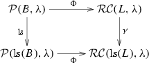
  commutes.

• (4) Suppose $B=B'\otimes B^{1,1}$. Let ${\text {rh}}(B)=B'$ with multiplicity array ${\text {rh}}(L)$. Then the diagram

  

  commutes.

• (4’) Suppose $B=B'\otimes B^{r,1}$ for $r=n-1$ or n. Let ${\text {rh}}_s(B)=B'$ with multiplicity array ${\text {rh}}_s(L)$. Then the diagram

  

  commutes.

• (5) Suppose $B=B'\otimes B^{r,1}$ with $2\le r\le n-2$. Let ${\text {rb}}(B)=B'\otimes B^{r-1,1}\otimes B^{1,1}$ with multiplicity array ${\text {rb}}(L)$. Then the diagram

  

  commutes.

• (6) Suppose $B=B'\otimes B^{r,s}$ with $s\ge 2$. Let ${\text {rs}}(B)=B'\otimes B^{r,s-1}\otimes B^{r,1}$ with multiplicity array ${\text {rs}}(L)$. Then the diagram

  

  commutes.

• (7) The diagram

  

  commutes.

Proof

For $B=B^{r_k,s_k}\otimes \cdots \otimes B^{r_2,s_2}\otimes B^{r_1,s_1}$, we set

$$\begin{aligned} \Vert B\Vert =\left( \sum _ir_is_i,\,\sum _i(r_i-1),\,\sum _i(s_i-1)\right) . \end{aligned}$$

We prove the statement by induction on the lexicographic order of $\Vert B\Vert$. More precisely, at each induction level, we check that $\Phi$ is well-defined from (1), (1’), (2), (3) and show that this $\Phi$ satisfies (4)—(7) for the next induction step.

The well-definedness of (1) is shown in [32].

The well-definedness of (1’) is shown in [38].

The well-definedness of (2) is shown in [38].

Now we prove the well-definedness of (3). When $B=B^{r,s}$ for $1\le r\le n-2$, the well-definedness of $\Phi$ and, in particular, (3) is established in [35, Theorem 5.9] by directly computing the bijection based on Proposition 3.9 and checking that the result agrees with the definition of the Kirillov–Reshetikhin tableau for the $I_0$-highest weight element of $B^{r,s}$. When $B=B^{r,s}$ for $r=n-1$ or n, both $\mathcal {P}(B^{r,s})$ and $\mathcal {RC}(L)$ consist of a single element and the property is easy to check.

For more general $B = B^{r,s} \otimes B'$ with $s\ge 2$, consider the following diagram:

We see that the left face and right face commute by definition and the back face commutes by the induction hypothesis that (7) holds. We wish to show that $(\Phi \circ {\text {ls}})(\mathcal {P}(B))\subseteq \gamma (\mathcal {RC}(L))$. If we have this relation, we can define $\Phi (\mathcal {P}(B))=(\gamma ^{-1}\circ \Phi \circ {\text {ls}})(\mathcal {P}(B))$ since $\gamma$ is invertible on $\mathrm {Im}(\gamma )$. Since $\diamond$ and $\theta$ are bijections, the commutativity of the left, back and right faces of the above diagram shows that it is enough to prove that $(\Phi \circ {\text {rs}})(\mathcal {P}(B^{\star }))\subseteq {\widetilde{\gamma }}(\mathcal {RC}(L))$.

Let us show $(\Phi \circ {\text {rs}})(\mathcal {P}(B))\subseteq {\widetilde{\gamma }}(\mathcal {RC}(L))$. For this, it is enough to check that the strings of $\nu ^{(r)}$ of the image of $\Phi \circ {\text {rs}}$ have strictly positive riggings. We prove this claim by dividing into cases.

When $B=B^{1,1}\otimes B'\otimes B^{r,s}$, consider the following diagram:

The front face commutes by already proved (1), the left face commutes by definition of ${\text {lh}}$ and ${\text {rs}}$, and the bottom face and the back face commute by induction hypothesis. There are two $\delta$ which we distinguish by denoting them by $\delta _1$ and $\delta _2$. By diagram chasing, we see that $(\delta _2\circ \Phi \circ {\text {rs}})(\mathcal {P}(B)) = ({\widetilde{\gamma }}\circ \delta _1\circ \Phi )(\mathcal {P}(B))$. Then by definition of ${\widetilde{\gamma }}$, we see that the algorithm for $\delta _1$ and $\delta _2$ choose the same strings and the only difference is the fact that, during the process of $\delta _2$, the riggings of the strings $\{(l, x) \in \bigl (\nu ^{(r)}, J^{(r)} \bigr ) \mid l < s\}$ are greater by 1 compared with the case of $\delta _1$. Since the riggings of the elements of $\mathcal {RC}(L)$ are nonnegative, we see that the riggings for the strings of $\nu ^{(r)}$ of the corresponding elements of $\mathcal {RC}({\text {rs}}(L))$ which are shorter than s are strictly positive. Therefore, we have $(\Phi \circ {\text {rs}})(\mathcal {P}(B))\subseteq {\widetilde{\gamma }}(\mathcal {RC}(L))$ in this case.

For $B=B^{r',1}\otimes B'\otimes B^{r,s}$ when $r'=n-1$ or n, the same arguments as above go through with $\delta$ and ${\text {lh}}$ replaced by $\delta _s$ and ${\text {lh}}_s$, respectively.

When $B=B^{r',1}\otimes B'\otimes B^{r,s}$ for $2\le r'\le n-2$, consider the following diagram:

The front face commutes by already proved (2), the left face commutes by definition of ${\text {lb}}$ and ${\text {rs}}$, and the bottom face and the back face commute by induction hypothesis. In this case, we have $(\beta _2\circ \Phi \circ {\text {rs}})(\mathcal {P}(B)) = ({\widetilde{\gamma }}\circ \beta _1\circ \Phi )(\mathcal {P}(B))$. Recall that $\beta$ does not change riggings of untouched strings. Therefore, by definition of ${\widetilde{\gamma }}$ we see that the riggings for strings of $\nu ^{(r)}$ of the elements of $\mathcal {RC}({\text {rs}}(L))$, which are shorter than s are greater by 1 compared with the corresponding elements of $\mathcal {RC}(L)$. Therefore, we have $(\Phi \circ {\text {rs}})(\mathcal {P}(B))\subseteq {\widetilde{\gamma }}(\mathcal {RC}(L))$ in this case.

Finally let us consider the case $B=B^{r',s'}\otimes B'\otimes B^{r,s}$. In this case, we have the following diagram:

The left face commutes by definition of ${\text {ls}}$ and ${\text {rs}}$, and the bottom face and the back face commute by induction hypothesis. In this case, we have $(\gamma \circ \Phi \circ {\text {rs}})(\mathcal {P}(B)) = ({\widetilde{\gamma }}\circ \Phi \circ {\text {ls}})(\mathcal {P}(B))$. Since $\gamma$ does not change any strings, we see that riggings for the strings of $\nu ^{(r)}$ of the elements of $\mathcal {RC}({\text {rs}}(L))$ which are shorter than s have strictly positive riggings. Therefore, we have $(\Phi \circ {\text {rs}})(\mathcal {P}(B))\subseteq {\widetilde{\gamma }}(\mathcal {RC}(L))$ in this case. This completes the proof of (3).

We move to the proof of (4). We again divide into cases.

When $B=B^{1,1}$, this follows from a special case of [38].

When $B=B^{1,1}\otimes B'\otimes B^{1,1}$, consider the following diagram:

(4.1)

The top face commutes by (1). The left face commutes by definition of ${\text {lh}}$ and ${\text {rh}}$, and the right face commutes by the fundamental relation $[\delta ,{\widetilde{\delta }}]=0$ (Theorem 3.11). The back and bottom faces commute by induction hypothesis. Since $\delta$ is injective, the front face commutes.

When $B=B^{r',1}\otimes B'\otimes B^{1,1}$ for $r'=n-1$ or n, we have the same commutative diagram as in (4.1) with ${\text {lh}}$ and $\delta$ replaced by ${\text {lh}}_s$ and $\delta _s$, respectively. The commutativity $[\delta _s, {\widetilde{\delta }}]=0$ is shown in Proposition 3.16 (i).

When $B=B^{r',1}\otimes B'\otimes B^{1,1}$ for $2\le r'\le n-2$, consider the following diagram and similarly show the front face commutes, using Proposition 3.12 (ii):

When $B=B^{r',s'}\otimes B'\otimes B^{1,1}$ consider the following diagram and similarly show the front face commutes, using Proposition 3.12 (iii):

The proofs of (5) and (6) are parallel to the argument of (4). When $B=B^{r,1}$, (5) follows from [38]. When $B=B^{r,s}$, (6) follows from Proposition 3.13 for $r\le n-2$, and from the fact that both $\mathcal {P}(B^{r,s})$ and $\mathcal {RC}(L)$ consist of a single element for $r=n-1,n$. We also need Propositions 3.12 and 3.16 (ii).

Case (4’) follows from cases (4) and (5) by noting that $\delta _s$ is realized by a composition of the doubling map, a sequence of n compositions of $\delta \circ \beta$, and a halving map.

Finally, we prove (7). We again divide into cases.

When $B=B^{1,1}\otimes B'$, we can use the following diagram to show that the front face commutes:

The proofs when $B=B^{r,1}\otimes B'$ or $B=B^{r,s}\otimes B'$ are almost the same. $\square$

We can now state the main result of this section.

Theorem 4.2

Let B be a tensor product of KR crystals. Then $\Phi :\mathcal {P}(B,\lambda ) \rightarrow \mathcal {RC}(L,\lambda )$ is a well-defined bijection.

Proof

By Proposition 4.1, $\Phi$ is a well-defined injection. By [5] or [27], we have $|\mathcal {P}(B,\lambda ) |= |\mathcal {RC}(L,\lambda ) |$, which proves that $\Phi$ is a bijection. $\square$

In order to generalize the rigged configuration bijection to include non-highest weight elements, we invoke the following result stated in [37, Thm. 4.1].

Theorem 4.3

([37]) The rigged configuration bijection $\Phi :\mathcal {P}(B) \rightarrow \mathcal {RC}(L)$ can be extended to a bijection $\Phi :B \rightarrow {\text {RC}}(L)$ by requiring $\Phi$ to be a classical crystal isomorphism:

$$\begin{aligned}{}[\Phi ,e_i]=[\Phi ,f_i]=0\qquad (i\in I_0). \end{aligned}$$

(4.2)

Example 4.4

Consider the rigged configuration $(\nu , J)$ in Example 3.2, $f_4(\nu , J)$ from Example 3.4, and the tensor product of KR crystal elements in Example 3.7. We have

5 ${{\varvec{R}}}$-invariance of rigged configurations

In this section, we prove that the combinatorial R-matrix on unrestricted rigged configurations is the identity under the bijection $\Phi$. We do so in several steps. First we show that the combinatorial R-matrix $R :B^{n,1} \otimes B^{r,s} \rightarrow B^{r,s} \otimes B^{n,1}$ corresponds to the identity map under $\Phi$ (see Proposition 5.7 which follows from Lemmas 5.2 and 5.5 and Proposition 5.6). The general statement (see Theorem 5.11) can then be deduced by passing a spin column through enough times to reduce to the type $A_n^{(1)}$ case which was proven in [21].

We begin with the R-matrix $R :B^{n,1}\otimes B^{r,s} \rightarrow B^{r,s} \otimes B^{n,1}$ for $1\le r\le n-2$ in type $D_n^{(1)}$. Let $b \otimes u_\eta \in B^{n,1}\otimes B^{r,s}$ be an $I_0$-highest weight element, where $u_\eta \in B(\eta ) \subseteq B^{r,s}$ is the unique $I_0$-highest weight element of highest weight $\eta$. Note that, for fixed $\eta$, the element $b\otimes u_\eta$ is uniquely specified by the weight $\lambda = {\text {wt}}(b\otimes u_\eta )$ since the multiplicity of any weight space in $B(\varpi _n) \cong B^{n,1}$ (as classical crystals) is at most 1.

Let us introduce the following notation. Write $\lambda = \sum _{i\in I_0} m_i \varpi _i$ in terms of the classical fundamental weights $\varpi _i$, where all $m_i$ are nonnegative integers since $\lambda$ is dominant. Define $\overline{\lambda } = \sum _{i \in I_0 {\setminus } \{n-1,n\}} m_i \varpi _i$. We can interpret $\overline{\lambda }$ as a partition (where each fundamental weight $\varpi _i$ for $1\le i\le n-2$ contributes a column of height i). Then let $\overline{\lambda }^c$ be the complement of the partition $\overline{\lambda }$ in the $r\times s$ rectangle. Similarly, $\eta ^c$ is the complement of $\eta$ (interpreted as a partition) in the $r\times s$ rectangle. The skew partition $\overline{\lambda }^c / \eta ^c$ can have at most one box in each row. Denote the cells in $\overline{\lambda }^c / \eta ^c$ from top to bottom (in English convention for partitions) by $c_1,c_2,\ldots ,c_\ell$. Finally, is obtained by replacing all of $\eta ^c$ by (recall that this is well-defined since $\eta$ is obtained from the $r\times s$ rectangle by removing vertical dominoes).

Note that $m_{n-1}+m_n=1$ due to the fact that $r\le n-2$ and $b \in B^{n,1}$. Also, $\ell +m_{n-1}$ is even since $b\in B^{n,1}$ (it would be odd for $b\in B^{n-1,1}$).

We now define the configuration that we will show under the bijection $\Phi$ corresponds to the $I_0$-highest weight elements $b \otimes u_\eta \in B^{n,1} \otimes B^{r,s}$ for $1\le r\le n-2$. Recall that $b\otimes u_\eta$ is uniquely determined by the two weights $\eta$ and $\lambda$. Let $\nu =\Gamma (\eta , \lambda )$ be the following configuration:

• (i) For $r\le a\le n-2$, $\nu ^{(a)}=\overline{\lambda }^c$.

• (ii) For $1\le a<r$, $\nu ^{(a)}$ is obtained from $\nu ^{(n-2)}$ by removing $r-a$ rows starting from longer rows.

• (iii) If $m_{n-1}=0$, then $\nu ^{(n-1)}$ (resp., $\nu ^{(n)}$) is obtained from by adding the cells $c_1, c_3,\ldots$ (resp., $c_2, c_4,\ldots$) to the same row length as in $\overline{\lambda }^c / \eta ^c$.If $m_{n-1}=1$, then $\nu ^{(n-1)}$ (resp., $\nu ^{(n)}$) is obtained from by adding the cells $c_2, c_4,\ldots$ (resp., $c_1, c_3,\ldots$) to the same row length as in $\overline{\lambda }^c / \eta ^c$.

Let us examine the vacancy numbers for elements $\nu \in \Gamma (\eta ,\lambda )$. It is not hard to check that $P_i^{(a)}(\nu )=0$ for all $1\le a \le n-2$ and $i\ge 0$. Furthermore, from weight considerations we have $P_i^{(n-1)}(\nu )=m_{n-1}$ and $P_i^{(n)}(\nu )=1-m_{n-1}$ for large i. Call $1\le h_1\le h_2 \le \cdots \le h_\ell$ the ordered row labels of the cells in and . Starting with the largest row in $\nu ^{(n-1)}$ (resp., $\nu ^{(n)}$), the vacancy number switches from 1 to 0 (or 0 to 1) whenever one of the row lengths $h_i$ is crossed. In particular, $P_i^{(n-1)}(\nu )+P_i^{(n)}(\nu )=1$ for all $i\ge 0$.

Example 5.1

We illustrate the construction of $\Gamma (\eta ,\lambda )$ with two examples. Consider type $D_{10}^{(1)}$ and $B = B^{10,1} \otimes B^{8,5}$. Let $b=(+,-,+,+,+,-,+,+,+,+)$ and

where $\eta = \varpi _2 + \varpi _6 + 3 \varpi _8$ and $\lambda = \varpi _1 + \varpi _5 + 3 \varpi _8 + \varpi _{10}$, and hence, $m_{10}=1$ and $m_9=0$. Thus, we have as partitions $\eta ^c = 221111$ and $\overline{\lambda }^c = 2221111$, and so

where we have indicated the cells $c_1$ and $c_2$ in the construction by blue letters 1 and 2, respectively. Then $\Phi (b \otimes u_{\eta })$ is equal to

where again we labelled the cells added to $\eta ^c$ in $\nu ^{(n-2)}$ and in $\nu ^{(n-1)}$ and $\nu ^{(n)}$ by blue letters 1 and 2.

Next we consider $b^\prime = (+,-,+,+,+,-,-,-,+,+)$ and $\mu {:}{=} {\text {wt}}(b' \otimes u_\eta )= \varpi _1 + \varpi _5 + \varpi _6 + 2\varpi _8 + \varpi _{10}$. Note that $\lambda \ne \mu$ and

Then $\Phi (b' \otimes u_{\eta })$ is

Lemma 5.2

Consider the $I_0$-highest weight element $b \otimes u_\eta \in B^{n,1}\otimes B^{r,s}$ of weight $\lambda$ with $1\le r\le n-2$, where $u_\eta$ is the $I_0$-highest weight element of highest weight $\eta$. Then the rigged configuration

$$\begin{aligned} (\nu ,J)=\Phi (b\otimes u_\eta ) \end{aligned}$$

satisfies $\nu = \Gamma (\eta ,\lambda )$ and $J^{(a)}_i=0$ for all $1\le a \le n-2$ and $i\ge 0$. $J_i^{(n-1)}$ and $J_i^{(n)}$ are determined as follows. Since $P_i^{(n-1)}(\nu )+P_i^{(n)}(\nu )=1$ either $J_i^{(n-1)}$ or $J_i^{(n)}$ can contain 1’s and the other riggings must be 0. The number of 1’s in $J_i^{(n-1)}$ (or $J_i^{(n)}$) is equal to the number of vertical dominoes in column i of $\overline{\lambda }^c/ \eta ^c$.

Proof

Let us define $d = {\text {emb}}(b)$. Let x be the letter in d at height h. Define $\delta ' = \beta ^{-1} \circ \delta ^{-1}$ unless $h = 1$ in which case $\delta ' = \delta ^{-1}$. Thus, $\delta '$ under the bijection $\Phi$ corresponds to adding the letter x to the step in the path using the algorithm for $\delta ^{-1}$, except we terminate after adding the last box to $(\nu ^{(h)}, J^{(h)})$. Let $w_i$ denote the row length of $\eta ^c$ corresponding to the row in $\overline{\lambda }^c/\eta ^c$ containing the cell $c_i$ as given in the construction $\Gamma (\eta , \lambda )$ (recall $\ell = |\overline{\lambda }^c/\eta ^c |$). Set $w_0 = \infty$ and $w_i = 0$ for all $i > \ell$. Define ${{\widetilde{w}}}_i = w_{\ell - i}$. In particular, we have $w_i \le w_{i+1}$ for all $0 \le i < \ell$. Define $\mu (x) = \#\{x \le x' \le n-2 \mid \overline{x}' \in d\}$.

First note that $\Phi (u_{\eta })$ is given by Proposition 3.9. Next we want to add b, which by the definition of $\delta _s$ involves the doubling map ${\text {emb}}$. Hence, we need to double $\Phi (u_{\eta })$. Denote the rigged configuration before having added the letter x by $(\overline{\nu }, \overline{J})$ and $(\overline{\nu }',\overline{J}') =\delta '(\overline{\nu }, \overline{J})$. Suppose we are adding the letter $x \le n-1$ to d at height h. $\square$

Claim

We obtain $\delta '(\overline{\nu }, \overline{J})$ from $(\overline{\nu },\overline{J})$ by adding a box to a (singular) string of length $2 {{\widetilde{w}}}_{a-h}$ to $\overline{\nu }^{(a)}$ for $h \le a < x$. Note that this is the $(a - h+1)$th cell from the bottom of $\overline{\lambda }^c / \eta ^c$. Moreover, all riggings are 0.

We prove the claim by induction on h. Suppose the letter y was added at height $h-1$ in the previous step (which might be vacuous if x is at height 1 in which case we set $y=0$). Note that $P_i^{(a)}(\overline{\nu }) > 0$ for all i such that $2 {{\widetilde{w}}}_{a-h} < i \le 2 {{\widetilde{w}}}_{a-h+1}$ and $h-1 \le a \le y<x$.

Observe that the number of minus signs appearing in b before position x is $x-h$. The application of $\delta '$ adds a box to the row of length $2{{\widetilde{w}}}_{x-h-1}$ in $\overline{\nu }^{(x-1)}$. This follows from the fact that no previous application of $\delta '$ changed $\overline{\nu }^{(x-1)}$ (our induction hypothesis), the description of $\overline{\nu }$ as given in Proposition 3.9, and that all rows strictly longer than $2 {{\widetilde{w}}}_{x-h-1}$ are non-singular. Next $\delta '$ adds a box to a row of length $2{{\widetilde{w}}}_{x-h-2}$ in $\overline{\nu }^{(x-2)}$ since all rows of length strictly between $2{{\widetilde{w}}}_{x-h-2}$ and $2{{\widetilde{w}}}_{x-h-1}$ are non-singular, $\overline{\nu }^{(x-2)}$ is the same as $\overline{\nu }^{(x-1)}$ with the top row removed, and we must select a row i such that $\overline{\nu }_i^{(x-2)} \le 2 {{\widetilde{w}}}_{x-h-1}$ by the definition of $\delta '$. A similar argument holds for $\overline{\nu }^{(a)}$ for the remaining $h \le a < x-1$ for the application of $\delta '$. From (3.1), the resulting riggings are all 0, and $P_i^{(a)}(\overline{\nu }') > 0$ for all i such that $2 {{\widetilde{w}}}_{a-h-1} < i \le 2 {{\widetilde{w}}}_{a-h}$ and $h \le a \le x$.

For $x = n, \overline{n}$, the application of $\delta '$ is similar to the above except we do not change $\overline{\nu }^{(n)}, \overline{\nu }^{(n-1)}$, respectively. Next suppose we are adding $\overline{x}$ at height h with $1\le x\le n-1$.

Claim

We obtain $\delta '(\overline{\nu }, \overline{J})$ from $(\overline{\nu },\overline{J})$ by the following steps:

• (i) add a box to the largest odd length string in $\overline{\nu }^{(a)}$ for $x \le a \le n-2$,

• (ii) for both $\overline{\nu }^{(n-1)}, \overline{\nu }^{(n)}$, either add to the largest odd length row or the row of length $2 w_{\mu (x)}$ depending on if there is an odd length row or not, respectively, and

• (iii) add a box to a row of length $2 {{\widetilde{w}}}_{a - h}$ in $\overline{\nu }^{(a)}$ for $h \le a < n-1$.

We prove the claim by using induction on $\overline{x}$ (i.e., as x decreases). Note that the largest singular row in $\overline{\nu }^{(x)}$ has length $2 w_{\mu (x)} + 1$, and it is the first row of $\overline{\nu }^{(x)}$.

By our induction assumption and the definition of $\delta '$, we add a box to a row of length $2 w_{\mu (x)} + 1$ in all $\overline{\nu }^{(a)}$ for $x \le a \le n-2$. Thus, step (i) follows. For step (ii), let $a = n-1,n$. Note that if there exists an odd length row, then from our induction, there is exactly one such row and it is of length $2 w_{\mu (x)} + 1$. Therefore, we add a box to this row. Otherwise all rows are currently of even length, so we add a box to a row of length $2 w_{\mu (x)}$. Note that $P_{2w_{\mu (x)}}^{(a)}(\overline{\nu }) = 0$ because we have only added boxes to $\overline{\nu }^{(n-2)}$ in rows of length at least $2w_{\mu (x)}$ (i.e., the resulting rows are strictly larger and don’t contribute to $P_{2w_{\mu (x)}}^{(a)}(\overline{\nu })$). The proof of step (iii) of the claim is similar to the proof of the previous claim for $x \le n - 2$.

From the aforementioned claims, it immediately follows that we obtain the desired configuration of $\Gamma (\eta , \lambda )$ after applying ${\text {emb}}^{-1}$.

Let us now turn to the statement about the riggings. A straightforward check from the above claim shows that all riggings are 0 in $\overline{\nu }^{(a)}$ for $a \le n - 2$. Next, each removable domino in $\overline{\lambda }^c/\eta ^c$ corresponds to two consecutive minus signs in b, which in turns corresponds to two barred letters $\overline{x}$ and $\overline{x+1}$. Note that when adding $\overline{x}$, the resulting vacancy number $P^{(a)}_{2 w_{\mu (x)}+2}(\overline{\nu }')=2$ for either $a=n-1$ or $a=n$ since the vertical domino implies we have an additional (as compared with $\Phi (u_{\eta })$) contribution of 6 boxes in $\overline{\nu }^{(n-2)}$, but only 2 boxes in $\overline{\nu }^{(a)}$. Hence, the corresponding rigging is 2. From the above description of $\delta '$, we do not change the corresponding row again when we add the remaining letters; thus, ${\text {emb}}^{-1}(\overline{\nu },\overline{J}) = \Phi (b \otimes u_\eta )$ is the desired rigged configuration. $\square$

Example 5.3

We consider $B = B^{8,1} \otimes B^{6,5}$ in type $D_8^{(1)}$ and fix $\lambda = \varpi _1 + 2 \varpi _6 + \varpi _7$. We now look at the set $\{ b \otimes u_{\eta } \in \mathcal {P}(B) \mid {\text {wt}}(b \otimes u_{\eta }) = \lambda \}$. We start with $\eta = \varpi _2 + 2 \varpi _6$ and $b = (+,-,+,+,+,+,+,-)$. Thus, we have

Next we consider $\eta ' = \varpi _4 + 2 \varpi _6$ and $b' = (+,-,-,-,+,+,+,-)$, and we have

Finally, we take $\eta '' = 3 \varpi _6$ and $b'' = (+,-,-,-,-,-,+,-)$, so that

Let us now turn our attention to $I_0$-highest weight elements in $B^{r,s} \otimes B^{n,1}$ for $1\le r\le n-2$ of weight $\lambda$. They are of the form $b \otimes u$ with $u{:}{=}u_{\varpi _n}=(+,\ldots ,+) \in B^{n,1}$ being (the unique) $I_0$-highest weight element and $b\in B(\mu ) \subseteq B^{r,s}$ for some $\mu$. Since $\varphi _i(u)=0$ for $1\le i\le n-1$ and $\varphi _n(u)=1$, we have that the part of b as a KN tableau without the letters n and $\overline{n}$ is highest weight of highest weight $\overline{\lambda }$ and the skew shape $\mu /\overline{\lambda }$ is a vertical strip. In b, the vertical strip $\mu /\overline{\lambda }$ contains the letter n and $\overline{n}$ in alternating order. Define $\eta$ as follows. In column i of b, let x be the number of removable n and $\overline{n}$ pairs and y the number of addable n and $\overline{n}$ pairs. Form a new tableau with the same $\overline{\lambda }$, but x and y interchanged for each column i. Then $\eta$ is the shape of this tableau.

Example 5.4

Consider type $D_{10}^{(1)}$ and

Thus, we have ${\text {wt}}(b \otimes u) = \lambda = \varpi _1 + \varpi _5 + \varpi _7 + \varpi _9$ and $\eta = \varpi _2 + \varpi _6 + \varpi _8$.

We use (4.2) in order to simplify the proof of the following lemma (instead of proving it directly using $\Phi$).

Lemma 5.5

Consider the $I_0$-highest weight element $b\otimes u\in B^{r,s}\otimes B^{n,1}$ of weight $\lambda$ with $1\le r\le n-2$ and $\eta$ as defined above. Then the rigged configuration

$$\begin{aligned} (\nu ,J) = \Phi (b \otimes u) \end{aligned}$$

is the same as in Lemma 5.2.

Proof

Recall that $\Phi (u)$ is the empty rigged configuration $\nu ^{(a)}=\emptyset$. Therefore, by the combinatorial procedure of $\Phi$, we see that the only difference between $\Phi (b\otimes u)$ and $\Phi (b)$ is that the riggings of $\nu ^{(n)}$ for the latter case is smaller than those for the former case by 1 since there is a contribution to the vacancy number by the tensor factor $B^{n,1}$ to $P_i^{(n)}(\nu )$. Thus, it is enough to show that for $({\widetilde{\nu }}, {\widetilde{J}})=\Phi (b)$, we have ${\widetilde{\nu }}=\Gamma (\eta ,\lambda )$ and ${\widetilde{J}}_i^{(a)}=0$ whenever $J_i^{(a)}=1$ in Lemma 5.2 and ${\widetilde{J}}_i^{(a)}=-1$ otherwise for $a=1,2$.

We are going to prove the lemma by induction on $|\mu /\overline{\lambda } |$. In fact, for simplicity we prove the statement simultaneously for the case stated as well as with all letters n and $\overline{n}$ as well as $u_{\varpi _n}$ and $u_{\varpi _{n-1}}$ interchanged. The claim for $\Phi (b\otimes u_{\varpi _{n-1}})$ is the same as in Lemma 5.2 with $(\nu ,J)^{(n-1)}$ and $(\nu ,J)^{(n)}$ interchanged. The base case $|\mu /\overline{\lambda } |= 0$ follows directly from Proposition 3.9.

Now suppose that $|\mu /\overline{\lambda } |> 0$ and assume that the topmost cell in $\mu /\overline{\lambda }$ is filled with $\overline{n}$ (resp., n). Suppose this cell is at height h. Consider

$$\begin{aligned} b' = e_h e_{h+1} \cdots e_{n-2} e_n (b) \qquad (\text {resp., } b' = e_h e_{h+1} \cdots e_{n-2} e_{n-1} (b)). \end{aligned}$$

Compared to b, the element $b'$ has a letter h instead of $\overline{n}$ (resp., n) in this cell, so that $\overline{\lambda }' = \overline{\lambda }+\epsilon _h$. Hence, by induction hypothesis $\Phi (b')$ is given as stated by the extension of the lemma. Furthermore, by Theorem 4.3 the Kashiwara operators $e_i$ and $\Phi$ commute, so that it suffices to check that

$$\begin{aligned} e_h e_{h+1} \cdots e_{n-2} e_n ({\widetilde{\nu }}, {\widetilde{J}}) \qquad (\text {resp., } e_h e_{h+1} \cdots e_{n-2} e_{n-1} ({\widetilde{\nu }}, {\widetilde{J}})) \end{aligned}$$

is indeed $({\widetilde{\nu }}',{\widetilde{J}}')=\Phi (b')$ as stated in the extension of the lemma. Recall the action of $e_i$ on rigged configurations as given in Definition 3.3. The smallest string with rigging -1 in $({\widetilde{\nu }},{\widetilde{J}})^{(n)}$ (resp., $({\widetilde{\nu }},{\widetilde{J}})^{(n-1)}$) is of length h, so that $e_n$ (resp., $e_{n-1}$) removes a box from this string. By the form of $({\widetilde{\nu }},{\widetilde{J}})$ as stated in the lemma, it is not hard to see that $e_{i+1} e_{i+2} \cdots e_{n-2} e_n({\widetilde{\nu }}, {\widetilde{J}})$ (resp., $e_{i+1} e_{i+2} \cdots e_{n-2} e_{n-1}({\widetilde{\nu }}, {\widetilde{J}})$) has a negative rigging $-1$ of smallest length in a string of length h in the ith rigged partition for each $h\le i \le n-2$. This shows that ${\widetilde{\nu }}^{'(n-2)} = (\overline{\lambda }')^{c}$ as required and all ${\widetilde{\nu }}^{'(a)}$ with $1\le a <n-2$ are as desired. The cells $c_1', c_2', \ldots$ in the construction of ${\widetilde{\nu }}^{'(n-1)}$ and ${\widetilde{\nu }}^{'(n)}$ are obtained from $(\overline{\lambda }')^c/(\eta ')^c$. There are two cases to consider:

• (1) $e_n$ (resp., $e_{n-1}$) removes one of the cells $c_i$ in $({\widetilde{\nu }},{\widetilde{J}})^{(a)}$ for $a=n$ (resp., $a=n-1$).

• (2) $e_n$ (resp., $e_{n-1}$) does not remove any of the cells $c_i$ in $({\widetilde{\nu }},{\widetilde{J}})^{(a)}$ for $a=n$ (resp., $a=n-1$).

Recall that the cells $c_j$ are those in $\overline{\lambda }^c/\eta ^c$ or alternatively $\eta /\overline{\lambda }$.

In Case (1), the cell containing the letter $\overline{n}$ (resp., n) at height h, which is also $c_i$, is part of $\eta$ and not part of a removable $(n,\overline{n})$-pair. Hence, $\eta '=\eta$. This implies that the list $c_1',c_2',\ldots$ is the same as the list $c_1,c_2,\ldots$, but with $c_i$ missing. If in the algorithm for $({\widetilde{\nu }},{\widetilde{J}})$, the cell $c_1$ is added to the ath rigged partition for $a=n-1$ or n, then in $({\widetilde{\nu }}',{\widetilde{J}}')$, the cell $c_1'$ is added to the opposite rigged partition. All addable $(n,\overline{n})$-pairs at height $<h$ come in pairs of the same row length. Hence, still cells are added to the same rows. The cell $c_i$ is missing from the list $c_j'$ and for $j\ge i$, $c_j'$ adds the same cell as $c_{j+1}$ to the same rigged partition, which proves the claim.

In Case (2), we have $\eta '=\eta +\epsilon _h+\epsilon _{h+1}$ since the $\overline{n}$ (resp., n) removed by the string of $e_j$ is part of a removable $(n,\overline{n})$-pair. Hence, $(\overline{\lambda }')^c/(\eta ')^c$ compared to $\overline{\lambda }^c/\eta ^c$ has an extra cell at height $h+1$, which implies that the sequence $c_j'$ compared to $c_j$ has an extra cell $c_i'$. As in Case (1), the cells at height $<h$ come in pairs and hence it does not matter whether one first adds them to the ath rigged partitions for $a=n-1$ or n or vice versa. Since $c_j'$ contains an extra cell $c_i$, $c_j'$ for $j>i$ adds the same cell as $c_{j-1}$ to the same rigged partition, which proves the claim. $\square$

To deal with the combinatorial R-matrices between two spin cases, we recall the following result by Mohammad [2].

Proposition 5.6

([2]) For $r = n-1, n$, the $I_0$-highest weight decomposition of $B^{n,1} \otimes B^{r,s}$ and $B^{r,s} \otimes B^{n,1}$ is multiplicity free. As a consequence, the combinatorial R-matrix

$$\begin{aligned} R :B^{n,1} \otimes B^{r,s} \rightarrow B^{r,s} \otimes B^{n,1} \end{aligned}$$

is uniquely determined by being an $I_0$-crystal isomorphism.

By combining these results, we now establish the R-invariance of the rigged configuration bijection for the case of $B^{n,1}\otimes B^{r,s}$ as follows:

Proposition 5.7

Consider an $I_0$-highest element $s_1 \otimes b_1$ of $B^{n,1}\otimes B^{r,s}$. Suppose that

$$\begin{aligned} R :s_1 \otimes b_1 \longmapsto b_2\otimes s_2\in B^{r,s}\otimes B^{n,1} \end{aligned}$$

under the combinatorial R-matrix. Then we have

$$\begin{aligned} \Phi (s_1\otimes b_1)=\Phi (b_2\otimes s_2). \end{aligned}$$

Proof

If $r = n-1,n$, this follows from Proposition 5.6 and Theorem 4.3.

Thus assume $r \le n-2$. By Lemmas 5.2 and 5.5, it suffices to show that under the combinatorial R-matrix, an $I_0$-highest weight element in $B^{n,1} \otimes B^{r,s}$ corresponding to the tuple $(\eta , \lambda )$ goes to the $I_0$-highest weight element in $B^{r,s} \otimes B^{n,1}$ with the same tuple $(\eta , \lambda )$ as given in the corresponding lemmas. We do so by induction on $|\lambda |$ (from largest to smallest) by either increasing $|\eta |$ or decreasing $|\eta /\overline{\lambda } |$.

Note that there is a unique element of weight $s\varpi _r+\varpi _n$ in both $B^{n,1} \otimes B^{r,s}$ and $B^{r,s} \otimes B^{n,1}$, so that $R(u_{\varpi _n} \otimes u_{s\varpi _r}) = u_{s\varpi _r} \otimes u_{\varpi _n}$. We set up the induction in several steps. Let $s_1 \otimes u_\eta \in B^{n,1} \otimes B^{r,s}$ be a highest weight element different from $u_{\varpi _n} \otimes u_{s\varpi _r}$. Perform one of the following steps to obtain a new $s_1' \otimes u_{\eta '}$ closer to $u_{\varpi _n} \otimes u_{s\varpi _r}$ by induction:

Step 1 Suppose $\varphi _0(s_1 \otimes u_\eta )>0$. Then let $s_1' \otimes u_{\eta '}$ be the $I_0$-highest weight element in the same component as $f_0(s_1 \otimes u_\eta )$.

Step 2 Suppose $\varphi _0(s_1 \otimes u_\eta )=0$. Note that in this case $\eta _1=s-1$ or s. Set $b_1 = u_\eta$ and repeat the following steps until $\varphi _0(s_1 \otimes b_1)>0$. Then let $s_1' \otimes u_{\eta '}$ be the $I_0$-highest weight element in the same component as $f_0 (s_1 \otimes b_1)$.

• (i) Let $1\le h < n-1$ be minimal such that $\varphi _h(s_1 \otimes b_1)>0$.

• (ii) Compute $s_1'\otimes b_1' = f_h(s_1\otimes b_1)$.

• (iii) Reset $s_1 \otimes b_1$ to $s_1' \otimes b_1'$.

Step 3 If neither Step 1 nor Step 2 applies or yields a $c=s_1 \otimes b_1$ with $\varphi _0(c)>0$, we have $\eta = (s-1) \varpi _r + \varpi _k$ for some $0\le k < r$ and $s_1=(+,\ldots ,+)$ or $(+,\ldots ,+,-,+,\ldots ,+,-)$ with one minus in position n and the other in position k or r. Note that, for fixed weight $\lambda$, these elements minimize $|\eta |$ and there is a unique $I_0$-highest weight element corresponding to $(\eta ,\lambda )$ with minimal $|\eta |$. On the $B^{r,s} \otimes B^{n,1}$ side, these are precisely the $I_0$-highest weight elements $b_2\otimes u_{\varpi _n}$ with $b_2 \in B(s\varpi _r) \subseteq B^{r,s}$ (since minimization of $|\eta |$ corresponds to maximization of $|\mu |$). Due to the uniqueness for a given weight class, they must map to each other under R.

We are now going to check for Steps 1 and 2 inductively, that if an $I_0$-highest weight element $s_1 \otimes u_\eta$ characterized by the tuple $(\eta ,\lambda )$ goes to $(\eta ',\lambda ')$ under a given step, then $b_2 \otimes u_{\varpi _n}$ corresponding to the same $(\eta ,\lambda )$ also goes to $(\eta ',\lambda ')$ under the same step.

We begin with Step 1. Suppose $f_0(s_1 \otimes u_\eta ) = s_1 \otimes f_0(u_\eta )$. Take $s_1 \otimes u_\eta$ of weight $\lambda$. By the combinatorial rules for $f_0$ on elements in $B^{r,s}$ provided in [40], we have that $\eta '$ (resp., $\lambda$) is $\eta$ (resp., $\lambda$) with a vertical domino added to rows 1 and 2. More precisely, $\eta _i'=\eta _i+1$ for $i=1,2$. Note also that $\eta _1<s$ (and in particular r even) and $\overline{\lambda }_1<\eta _1$ if $\eta _1=s-1$ since otherwise $f_0$ does not apply. Now take $b_2 \otimes u_{\varpi _n}$ corresponding to $(\eta ,\lambda )$ with $b_2\in B(\mu )$. The action of $f_0$ is given by Lemma 2.4. If case Lemma 2.4(i) applies, we have $\mu _i = \eta _i = \overline{\lambda }_i+1$ and $\eta _i'=\mu _i'+1= \overline{\lambda }_i'+1$ for $i=1,2$, so that indeed $\eta _i'=\eta _i+1$. Lemma 2.4(ii) does not apply since r cannot be odd. If Lemma 2.4(iii) applies, we have $\mu _i=\overline{\lambda }_i+1=\eta _i+1$ and $\mu _i'=\overline{\lambda }'_i+1=\eta '_i+1$ with $\mu _i'=\mu _i+1$ for $i=1,2$, so that again $\eta _i'=\eta _i+1$. This proves the claim for Step 1 with $f_0(s_1 \otimes u_\eta ) = s_1 \otimes f_0(u_\eta )$.

Step 1 with $f_0(s_1 \otimes u_\eta ) = f_0(s_1) \otimes u_\eta$ can only apply when $\eta _1=s$ and $s_1$ has − in positions 1 and 2. Under $f_0$ these two minus in $s_1$ are turned into $+$, so that $\lambda _i'=\lambda _i+1$ for $i=1,2$, $\lambda _i'=\lambda _i$ for $i\ge 3$, and $\eta '=\eta$. When r is even, the correspondence gives $\mu _i=\overline{\lambda }_i=s-1$ for $i=1,2$. Then Lemma 2.4(iii) applies and yields $\mu _i'=s=\overline{\lambda }_i'=\eta _i'$ for $i=1,2$ as desired. When r is odd, the correspondence yields $\eta _1=s$, $\overline{\lambda }_1=s-1$, and $\mu _1=s$. Lemma 2.4(i) or (ii) applies, and it can again be easily checked that $\eta '=\eta$, proving Step 1 with $f_0(s_1 \otimes u_\eta ) = f_0(s_1) \otimes u_\eta$.

Next consider Step 2. The algorithm of always picking the smallest applicable $f_h$ and applying it has the following effect on $s_1 \otimes u_\eta$. It raises the entries in the shortest columns of $u_\eta$ and/or lowers the lowest minus signs in $s_1$ until $f_0$ is applicable. We are going to consider several cases:

• (a) No minus sign in $s_1$ moves to positions 1 and 2.

• (b) Only one minus sign in $s_1$ moves to position 1 or 2.

• (c) Two minus signs in $s_1$ move to positions 1 and 2.

First consider Case (a). Note that $\varepsilon _0(s_1)=1$, so that the sequence of $f_h$ must raise the entries in at least the two shortest columns in order to achieve $\varphi _0(s_1 \otimes u_\eta )>0$. Let $h_1 \le h_2<r$ be the height of the two rightmost columns in $\eta$. Then the algorithm for Step 2 adds a vertical domino to the leftmost column of height $h_2$ in $\eta$ and does the same to $\overline{\lambda }$. On the other side $b_2 \otimes u_{\varpi _n}$ with $b_2 \in B(\mu )$, the subpart of $b_2$ of shape $\overline{\lambda }$ is a tableau with i in row i, whereas $\mu /\overline{\lambda }$ is filled with the letters n and $\overline{n}$. Since we only apply $f_h$ with $1\le h\le n-2$, the letters n and $\overline{n}$ never change in $b_2$. By the correspondence between $(\eta ,\lambda )$ and $\mu$ as described before Example 5.4, the vertical strip $\mu /\overline{\lambda }$ has boxes at height h with $h_1< h \le h_2$ and $b_2$ contains letters n and $\overline{n}$ in these cells. The steps in the algorithm add a vertical strip at height $h_2$ to $\overline{\lambda }$ and as a consequence push any letters n and/or $\overline{n}$ at height $h_2+1$ and $h_2+2$ one column to the right. Hence, $\mu '=\mu +\epsilon _{h_2+1}+\epsilon _{h_2+2}$ which implies that the correspondence between $(\eta ',\lambda ')$ and $\mu '$ also holds, proving the claim.

Next consider Case (b). Let $h_1 \le h_2<r$ again be the height of the two rightmost columns in $\eta$. The spin column $s_1$ must have precisely one minus sign in position $1\le h \le h_2$, which is either in position $h_1$ or position $h_2$. First consider that it is in position $h_2>h_1$. Then the algorithm for Step 2 adds a vertical domino to the column of height $h_1$ in $\eta$ and moves the minus sign in $s_1$ from position $h_2$ to position $h_1+2$. This means $\eta '=\eta +\epsilon _{h_1+1} +\epsilon _{h_1+2}$ and $\overline{\lambda }' = \overline{\lambda } + \epsilon _{h_2} + \epsilon _{h_1+1}$. On the $b_2 \otimes u_{\varpi _n}$ side, the vertical strip $\mu /\overline{\lambda }$ has boxes at heights $h_1<h\le h_2-2$ and $h_2$. The algorithm for Step 2 on this side again changes $\overline{\lambda }'=\overline{\lambda } + \epsilon _{h_2} + \epsilon _{h_1+1}$. The letters n and $\overline{n}$ in $b_2$ in the rightmost column move up one, and the letter $\overline{n}$ at height $h_2$ moves from the second to last to last column. This implies $\eta '=\eta +\epsilon _{h_1+1} +\epsilon _{h_1+2}$ as before, proving the claim.

Next consider Case (b) with a minus in $s_1$ at height $h_1 \le h_2<r$. In this case, the algorithm for Step 2 adds a vertical domino at height $h_2$ to $\eta$ and $\overline{\lambda }$, so that $\eta '=\eta +\epsilon _{h_2+1} + \epsilon _{h_2+2}$ and $\overline{\lambda }'=\overline{\lambda } +\epsilon _{h_2+1} + \epsilon _{h_2+2}$. On the $b_2 \otimes u_{\varpi _n}$ side, the vertical strip $\mu /\overline{\lambda }$ has boxes at heights $h_1\le h\le h_2$. The algorithm for Step 2 also changes $\overline{\lambda }'=\overline{\lambda } +\epsilon _{h_2+1} + \epsilon _{h_2+2}$ and pushes any n and $\overline{n}$ at height $h_2+1$ and $h_2$ one column to the right. This implies that indeed $\eta '=\eta +\epsilon _{h_2+1} + \epsilon _{h_2+2}$ as desired.

Finally consider Case (c). In this case, there must be at least two minus signs in $s_1$ in positions $1\le i \le h_2$, where $h_1\le h_2<r$ are again the heights of the rightmost columns in $\eta$. The algorithm for Step 2 removes the lowest two minus signs in $s_1$. Let $i_1<i_2$ be the positions of these two minus signs. Then $\overline{\lambda }'=\overline{\lambda }+\epsilon _{i_1}+\epsilon _{i_2}$ and $\eta '=\eta$. On the $b_2 \otimes u_{\varpi _n}$ side, the vertical strip $\mu /\overline{\lambda }$ has boxes at height $i_1\le i \le i_2-2$ and $i_2$ if $i_1\le i_2-2$ and at height $i_1$ and $i_1+1$ if $i_2=i_1+1$. The algorithm of Step 2 also changes $\overline{\lambda }'=\overline{\lambda }+\epsilon _{i_1}+\epsilon _{i_2}$. In addition, it moves the letters n and $\overline{n}$ in $b_2$ up by one in the last column of $b_2$ and n at height $i_2$ one column to the right if $i_1\le i \le i_2-2$. When $i_2=i_1+1$, it moves the letters n and $\overline{n}$ in the last column of $b_2$ up by two. Comparing $\mu '$ and $\overline{\lambda }'$ shows that indeed $\eta '=\eta$ as desired. $\square$

Finally, we prepare the following proposition to prove the R-invariance. Let $u\in B^{n,1}$ be the $I_0$-highest weight element. For $b\in B$, we define $\mathbb {T}(b)$ by $R(b\otimes u)=u'\otimes \mathbb {T}(b)$. Here we view $\mathbb {T} :B \rightarrow B$ as an operator by passing through u via the combinatorial R-matrix.

Proposition 5.8

Suppose $r_2\le r_1$. Let $b_2\otimes b_1\in B^{r_2,s_2}\otimes B^{r_1,s_1}$ be an $I_0$-highest weight element. Then there exists an integer N such that $\mathbb {T}^N(b_2\otimes b_1)$ belongs to $B(s_2\varpi _{r_2})\otimes B(s_1\varpi _{r_1})$ and the right factor is the $I_0$-highest weight element. Moreover,

• (i) if $r_2\le n-2$ and $r_1\le n-1$, then the left factor does not contain barred letters;

• (ii) otherwise, the left factor is the $I_0$-highest weight element.

Proof

We first assume $r_1,r_2\le n-2$. Suppose $b_2\otimes b_1\in B^{r_2,s_2}\otimes B^{r_1,s_1}$ is $I_0$-highest weight. Then $b_1=u_\mu$ where $u_\mu$ is the $I_0$-highest weight element of $B(\mu )\subset B^{r_1,s_1}$. In view of the description of the combinatorial $R:B^{r_1,s_1}\otimes B^{n,1}\rightarrow B^{n,1}\otimes B^{r_1,s_1}$ in terms of the pairs $(\eta ,\lambda )$ as described in the proof of Proposition 5.7, successive applications of R take this $u_\mu$ to $u_{s_1\varpi _{r_1}}$. Thus, we can assume $b_1=u_{s_1\varpi _{r_1}}$ and

$$\begin{aligned} e_i^{s_1\delta _{i,r_1}+1}b_2=0\text { for }i\in I_0. \end{aligned}$$

(5.1)

We also know $R(u_{s_1\varpi _{r_1}}\otimes u)=u\otimes u_{s_1\varpi _{r_1}}$. So we consider $R(b_2\otimes u)$ next. Consider $\mathrm {high}(b_2\otimes u)$. The left component may contain $n,\overline{n}$ pairs. If so, $R:B^{r_2,s_2}\otimes B^{n,1}\rightarrow B^{n,1}\otimes B^{r_2,s_2}$ removes them. Therefore, we can assume that there do not exist any $n,\overline{n}$ pairs. Once all $n,\overline{n}$ pairs are removed, suppose $b_2 \in B(\lambda )$. Then the right component of $R(b_2\otimes u)$ belongs to $B(\lambda ')$, where $\lambda '$ is strictly greater than $\lambda$ in the dominance order. Hence, we can assume $\lambda =s_2\varpi _{r_2}$. From (5.1), the first barred letter in the inverse column reading word of $b_2$ is $\overline{r}_1$. Let $R(b_2\otimes u)=c\otimes {\widetilde{b}}_2\in B^{n,1}\otimes B^{r_2,s_2}$. Since c contains a −, the number of barred letters in ${\widetilde{b}}_2$ is at least one smaller than that of $b_2$. Therefore, the claim follows.

A similar argument when $r_2\le n-2$ and $r_1=n-1$ finishes the proof of (i). Case (ii) is easier. $\square$

Example 5.9

Consider type $D_8^{(1)}$, $B = B^{4,4} \otimes B^{6,3}$ and

Then we have

where $u'$ is defined by $R(b\otimes u)=u'\otimes \mathbb {T}(b)$ with $b=b_2 \otimes b_1$. This illustrates Case (i) of Proposition 5.8.

Example 5.10

Consider type $D_8^{(1)}$, $B = B^{4,4} \otimes B^{8,3}$ and

Then we have

This illustrates Case (ii) of Proposition 5.8.

The following property is one of the most profound properties of the rigged configuration bijection.

Theorem 5.11

(R-invariance) Let $B=B^{r_k,s_k}\otimes \cdots \otimes B^{r_2,s_2}\otimes B^{r_1,s_1}$ and let $B'$ be an arbitrary reordering of the factors of B. For a given element $b\in B$, suppose that $b'\in B'$ is isomorphic to b under the combinatorial R-matrix:

$$\begin{aligned} R :b\cong b'. \end{aligned}$$

Then the corresponding unrestricted rigged configurations are invariant:

$$\begin{aligned} \Phi (b)=\Phi (b'). \end{aligned}$$

Proof

We divide the proof into three steps.

Step 1 By Theorem 4.3, we can assume that b is an $I_0$-highest weight element. Suppose that $b=b_k\otimes b_{k-1}\otimes b_{k-2}\otimes \cdots \otimes b_1\in B$. By the recursive structure of the algorithm of the rigged configuration bijection $\Phi$, we see that it is enough to consider the case $b'={\widetilde{b}}_{k-1}\otimes {\widetilde{b}}_k\otimes b_{k-2}\otimes \cdots \otimes b_1$, where $R :b_k\otimes b_{k-1} \cong {\widetilde{b}}_{k-1}\otimes {\widetilde{b}}_k$. Then the relationship between the $\diamond$ duality and the $\theta$ operation established in Proposition 4.1(7) shows that it is enough to consider the case $k=2$. Therefore, we concentrate on the case when $b=b_2\otimes b_1$ is $I_0$-highest weight.

Step 2 Let $u\in B^{n,1}$ be the $I_0$-highest weight element and $b=b_2 \otimes b_1 \in B$ be $I_0$-highest weight. We shall show that

$$\begin{aligned} \Phi (b\otimes u)=\Phi (u'\otimes \mathbb {T}(b)), \end{aligned}$$

(5.2)

where $R :b\otimes u\cong u'\otimes \mathbb {T}(b)$. By Proposition 5.7, we have

$$\begin{aligned} \Phi (b_2\otimes b_1\otimes u)=\Phi (b_2\otimes u''\otimes b_1'), \end{aligned}$$

where $R :b_1\otimes u\cong u''\otimes b_1'$. Then by Proposition 4.1(7), we have

$$\begin{aligned} \Phi (\widehat{u}\otimes \widehat{b}_1 \otimes \widehat{b}_2) = \Phi (\widehat{b}_1' \otimes \widehat{u}'' \otimes \widehat{b}_2), \end{aligned}$$

where $(b_2\otimes b_1\otimes u)^{\diamond } = \widehat{u} \otimes \widehat{b}_1 \otimes \widehat{b}_2$ and $(b_2\otimes u''\otimes b_1')^{\diamond } = \widehat{b}_1' \otimes \widehat{u}'' \otimes \widehat{b}_2$. Since $\widehat{u}'' \in B^{n,1}$, again by Proposition 5.7 we have

$$\begin{aligned} \Phi (\widehat{b}_1' \otimes \widehat{u}'' \otimes \widehat{b}_2)= \Phi (\widehat{b}_1' \otimes \widehat{b}_2' \otimes \widehat{u}'), \end{aligned}$$

where $R :\widehat{u}'' \otimes \widehat{b}_2 \cong \widehat{b}_2' \otimes \widehat{u}'$. Note that $(\widehat{b}_1' \otimes \widehat{b}_2' \otimes \widehat{u}')^{\diamond } = u'\otimes \mathbb {T}(b)$ since $\diamond$ is involutive. Therefore by Proposition 4.1(7), we obtain (5.2).

Step 3 Let $b_2\otimes b_1\in B$ be $I_0$-highest weight and $R(b_2\otimes b_1)=\tilde{b}_1\otimes \tilde{b}_2$. Then we have

$$\begin{aligned} b_2\otimes b_1\otimes u\simeq u'\otimes \mathbb {T}(b_2\otimes b_1) \text { and } \tilde{b}_1\otimes \tilde{b}_2\otimes u\simeq u'\otimes \mathbb {T}(\tilde{b}_1\otimes \tilde{b}_2). \end{aligned}$$

Thus by Step 2, we have

$$\begin{aligned} \Phi (b_2\otimes b_1\otimes u)=\Phi (u'\otimes \mathbb {T}(b_2\otimes b_1)) \text { and } \Phi (\tilde{b}_1\otimes \tilde{b}_2\otimes u)=\Phi (u'\otimes \mathbb {T}(\tilde{b}_1\otimes \tilde{b}_2)). \end{aligned}$$

Since $\Phi (b_2\otimes b_1\otimes u)=\Phi (\tilde{b}_1\otimes \tilde{b}_2\otimes u)$ is equivalent to $\Phi (b_2\otimes b_1)=\Phi (\tilde{b}_1\otimes \tilde{b}_2)$, the claim is reduced to showing $\Phi (\mathbb {T}(b_2\otimes b_1))=\Phi (\mathbb {T}(\tilde{b}_1\otimes \tilde{b}_2))$. Thanks to Proposition 5.8, we are left to show $\Phi (b_2\otimes b_1)=\Phi (\tilde{b}_1\otimes \tilde{b}_2)$ when either $b_2\otimes b_1$ or $\tilde{b}_1\otimes \tilde{b}_2$ has the property described in the proposition. If $r_1,r_2\le n-2$, this R-matrix is nothing but type A by [24, Proposition 9.1] and the R-invariance of type A case is already treated in [21, Lemma 8.5]. If $r_1=n$, by Proposition 5.8 both factors are $I_0$-highest weight and the images of $\Phi$ are empty. When $r_1=n-1$, then by symmetry we can interchange in all arguments $n-1$ and n (including in the definition of $\mathbb {T}$), so that this case reduces to the $r_1=n$ case. $\square$

Theorem 5.11 means that the rigged configuration bijection gives an explicit algorithm to compute the combinatorial R-matrices. It is noteworthy that the rigged configuration bijection gives not only the combinatorial R-matrices for twofold tensor products but also much more general reorderings of multiple tensor products by only computing $\Phi$ and $\Phi ^{-1}$. In the following, we give one such example.

Example 5.12

Consider the following element of $B=B^{3,3}\otimes B^{2,4}\otimes B^{2,2}$ of type $D^{(1)}_5$:

The corresponding unrestricted rigged configuration is

From this unrestricted rigged configuration, we can obtain the image in $B'=B^{2,2}\otimes B^{2,4}\otimes B^{3,3}$ as follows:

Then by Theorem 5.11, we have $R:b\cong b'$. In this way, we can obtain the combinatorial R-matrices as $R=\Phi ^{-1}_{B'}\circ \Phi _B$.

6 Energy function and fermionic formula

6.1 Involution $\varsigma$ and energy function

In [23], the involution $\varsigma$ on $B^{r,s}$ ($1\le r\le n-2,s\ge 1$) was shown to exist, which is the unique map satisfying

$$\begin{aligned} \varsigma (e_ib)&= e_{n-i}\varsigma (b), \end{aligned}$$

(6.1a)

$$\begin{aligned} \varsigma (f_ib)&=f_{n-i}\varsigma (b), \end{aligned}$$

(6.1b)

for any $i\in I,b\in B^{r,s}$. We need the following lemma later.

Lemma 6.1

For $u_\lambda \in B(\lambda )\subseteq B^{r,s}$, $\varsigma (u_\lambda )$ belongs to $B(s\varpi _r)$ and is given as follows. To $\lambda$ associate a tuple $\mu =(\lambda '_s,\lambda '_{s-1},\ldots , \lambda '_1,r,\ldots ,r)$ with 2s entries, where $\lambda '$ is the transpose of the partition $\lambda$. Denote the jth entry of $\mu$ by $\mu _j$. Let t be the KN tableau for $\varsigma (u_\lambda )$. Then the kth column of t is given by

$$\begin{aligned} \overline{n-\mu _{2k-1}+1} \cdots \overline{n-1} \overline{n} n \cdots n \overline{n} (n - \mu _{2k}) \cdots (n-r+2) (n-r+1). \end{aligned}$$

Proof

Since $u_\lambda$ is the unique element of $B^{r,s}$ of weight $\lambda$ satisfying $e_iu_\lambda =0$ for $i=1,\ldots ,n$, the element $\varsigma (u_\lambda )$ should be the unique element of $-w^{A_{n-1}}_0\lambda$ satisfying $e_i\varsigma (u_\lambda )=0$ for $i=0,1,\ldots ,n-1$, where $w^{A_{n-1}}_0$ is the longest element of the Weyl group of $A_{n-1}\subseteq D_n$. One checks that t is an allowed KN tableau [16] of the desired weight. Hence, it is sufficient to show that $e_it=0$ for $i=0,1,\ldots ,n-1$. For $i=1,\ldots ,n-1$, this is immediate. To see $e_0t=0$, calculate the $\{2,\ldots ,n\}$-highest weight element in the same component as t, which is the tableau whose columns are all $23\cdots r+1$, and hence $\sigma (t)=t$ with $\sigma$ as in (2.8). In view of the definition of $e_0$ given in (2.10), we have $e_0t=0$, since $e_1t=0$. $\square$

We need an involution $\varsigma$ also on $B^{n-1,s}$ and $B^{n,s}$. When n is odd, it becomes a map from $B^{n-1,s}$ to $B^{n,s}$ and vice versa. To incorporate this situation, we introduce $\eta$ defined to be 0 if n is even and 1 otherwise. Then there exists a map $\varsigma :B^{n-1,s} \rightarrow B^{n-1+\eta ,s}$ (resp., $B^{n,s} \rightarrow B^{n-\eta ,s}$) satisfying (6.1). In fact, it is characterized by (6.1) and defining the image of $u_{s\varpi _{n-1}}$ (resp., $u_{s\varpi _n}$) to be the unique element in $B^{n-1+\eta ,s}$ (resp., $B^{n-\eta ,s}$) of weight $-w^{A_{n-1}}_0(s\varpi _{n-1})$ (resp., $-w^{A_{n-1}}_0(s\varpi _n)$).

For a multiple tensor product of KR crystals $B=B^{r_k,s_k}\otimes \cdots \otimes B^{r_1,s_1}$, we define

$$\begin{aligned} \varsigma (b)=\varsigma (b_k)\otimes \cdots \otimes \varsigma (b_1) \end{aligned}$$

for $b=b_k\otimes \cdots \otimes b_1\in B$

Proposition 6.2

For any $I_0$-highest weight element $u_\lambda$ of a single KR crystal $B^{r,s}$, we have $({\text {rs}}\circ \varsigma )(u_\lambda )=(\varsigma \circ {\text {rs}})(u_\lambda )$.

Proof

The case when $r=n-1$ or n is straightforward. Both ${\text {rs}}\circ \varsigma$ and $\varsigma \circ {\text {rs}}$ send $u_{s\varpi _{n-1}}$ (resp., $u_{s\varpi _n}$) to $v_{-(s-1)w_0\varpi _{n-1}}\otimes v_{-w_0\varpi _{n-1}}$ (resp., $v_{-(s-1)w_0\varpi _n}\otimes v_{-w_0\varpi _n}$) where $w_0$ is the longest element of $A_{n-1}\subseteq D_n$ and $v_\tau$ stands for the unique element in the crystal of weight $\tau$.

Suppose $r\le n-2$. In this case, $({\text {rs}}\circ \varsigma )(u_\lambda )$ is given by cutting the rightmost column of $\varsigma (u_\lambda )$. From Proposition 2.6, we see ${\text {rs}}(u_\lambda )=t\otimes u_{\varpi _r}$, where the tableau t is described in the proposition. We use all the notation for t from Proposition 2.6. Hence, $(\varsigma \circ {\text {rs}})(u_\lambda )=\varsigma (t)\otimes \varsigma (u_{\varpi _r})$. By Lemma 6.1, the right components of $({\text {rs}}\circ \varsigma )(u_\lambda )$ and $(\varsigma \circ {\text {rs}})(u_\lambda )$ agree. We prove that the left components also agree by decreasing induction on p, where p is as in Proposition 2.6 for t. If $p=r$, the claim is true, since in this case t is $I_0$-highest weight and the agreement can be shown by Lemma 6.1. Suppose $p<r$. Let $t'$ be the tableau that differs from t only in the first column with $\overline{p+1} \cdots \overline{r-1} \overline{r} q \cdots 21$ replaced by $\overline{p+3} \cdots \overline{r-1} \overline{r} q \cdots 21$. These tableaux are connected in the crystal graph as $t'=e_{\mathbf{a}_2}f_0f_{\mathbf{a}_1}t$ where

$$\begin{aligned} \mathbf{a}_1&=\mathbf{b}(2,1+\mu _{\ge 2})\cdots \mathbf{b}(p-2,1+\mu _{\ge p-2}) \mathbf{b}(p,1+\mu _{\ge p}),\\ \mathbf{a}_2&=\mathbf{b}(p,\mu _{\ge p})\cdots \mathbf{b}(4,\mu _{\ge 4})\mathbf{b}(2,\mu _{\ge 2}), \end{aligned}$$

$\mathbf{b}(j,a)=j^a(j-1)^a(j+1)^aj^a$ and $\mu _{\ge c}=\sum _{j=c}^{\ell (\mu )}\mu _j$. (See (2.9) for the definition of $e_{\mathbf{a}}$. The definition of $f_{\mathbf{a}}$ is similar.) In fact, the tableau $f_{\mathbf{a}_1}t$ has the following form. The first column is

$$\begin{aligned} \overline{1}\,\overline{2}\,\overline{p+3}\cdots \overline{r-1}\, \overline{r}\, (q+2) \cdots 43, \end{aligned}$$

and the entries in the other part of t are shifted by 2. Thus, $f_0$ removes $\overline{1}\,\overline{2}$ from the first column.

Since $\varsigma (e_{\mathbf{a}_2}f_0f_{\mathbf{a}_1}t)=e_{n-\mathbf{a}_2}f_nf_{n-\mathbf{a}_1}t$, where for $\mathbf{a}=a_1\cdots a_m$, $n-\mathbf{a}$ stands for $(n-a_1)\cdots (n-a_m)$, we are left to show that $e_{n-\mathbf{a}_2}f_nf_{n-\mathbf{a}_1}t$ agrees with the first $s-1$ columns of $\varsigma (u_\lambda )$ of Lemma 6.1 with $\lambda '_1$ replaced by $\lambda '_1+2$. This can be checked directly. $\square$

In Sect. 2.6, we defined the combinatorial R-matrix $R :B^{r_2,s_2}\otimes B^{r_1,s_1} \rightarrow B^{r_1,s_1}\otimes B^{r_2,s_2}$. In addition, there exists a function $\overline{H} :B^{r_2,s_2}\otimes B^{r_1,s_1}\rightarrow \mathbb {Z}$, called the local energy function, unique up to a global additive constant. It is constant on $I_0$-components and satisfies for all $b_2\in B^{r_2,s_2}$ and $b_1\in B^{r_1,s_1}$ with $R(b_2\otimes b_1)=b_1'\otimes b_2'$

$$\begin{aligned} \overline{H}(e_0(b_2\otimes b_1))= \overline{H}(b_2\otimes b_1)+ {\left\{ \begin{array}{ll} 1 &{} \text {if }\varepsilon _0(b_2)>\varphi _0(b_1)\text { and } \varepsilon _0(b_1')>\varphi _0(b_2'), \\ -1 &{} \text {if }\varepsilon _0(b_2)\le \varphi _0(b_1)\text { and } \varepsilon _0(b_1')\le \varphi _0(b_2'), \\ 0 &{} \text {otherwise.} \end{array}\right. } \end{aligned}$$

(6.2)

We shall normalize the local energy function by the condition $\overline{H}(u_{s_2\varpi _{r_2}}\otimes u_{s_1\varpi _{r_1}})=0$.

For a crystal $B^{r,s}$, the intrinsic energy $\overline{D}_{B^{r,s}} :B^{r,s}\rightarrow \mathbb {Z}$ is defined as follows. When $r\le n-2$, we define $\overline{D}_{B^{r,s}}(b)=(rs - |\lambda |)/2$ for $b\in B(\lambda )\subseteq B^{r,s}$ (see (2.6)). When $r=n-1,n$, there is only one $I_0$-component (see (2.7)) and we set $\overline{D}_{B^{r,s}}(b)=0$ for $b\in B^{r,s}$. On the tensor product $B=B_k\otimes \cdots \otimes B_1$ of single KR crystals $B_j$, there is an intrinsic energy function $\overline{D}_B :B\rightarrow \mathbb {Z}$ defined in [9, (3.8)] and [33, Section 2.14] by

$$\begin{aligned} \overline{D}_B = \sum _{1 \le i < j \le k} \overline{H}_i R_{i+1} R_{i+2}\cdots R_{j-1} + \sum _{j=1}^k \overline{D}_{B_j} \pi _1 R_1 R_2 \cdots R_{j-1}. \end{aligned}$$

(6.3)

Here $R_i$ and $\overline{H}_i$ denote the combinatorial R-matrix and local energy function, respectively, acting on the ith and $(i+1)$th tensor factors counting from the right. Also $\pi _1$ is the projection onto the rightmost tensor factor. The intrinsic energy $\overline{D}_B$ is constant on any $I_0$-component of B. Let $B'$ be the same tensor product of KR crystals as B except that the ith and $(i+1)$th positions are interchanged. Let $b'=b'_k\otimes \cdots \otimes b'_1\in B'$ be such that $b'_{i+1}\otimes b'_i=R(b_{i+1}\otimes b_i)$ and $b'_j=b_j$ for $j\ne i,i+1$. Then we have $\overline{D}_B(b)=\overline{D}_{B'}(b')$. Similarly, let $B'$ be any reordering of the tensor factors of B. The image $b'$ of b under the compositions of the combinatorial R-matrices does not depend on the order of applications due to the Yang–Baxter equation, and we also have $\overline{D}_B(b)=\overline{D}_{B'}(b')$, see [9, Prop. 3.9] and [33, Prop. 2.15]. In what follows we often drop the subscript B from $\overline{D}_B(b)$.

In [23, 24], we proved the following formula on the intrinsic energy $\overline{D}$ under the assumption that the KR crystals $B^{r_j,s_j}$ appearing in B satisfy $r_j\le n-2$.

Proposition 6.3

([23, 24]) For an $I_0$-highest weight element b in B, we have

$$\begin{aligned} \overline{D}(b)=\overline{D}(\varsigma (b))+\frac{|B |- |\lambda (b) |}{2}, \end{aligned}$$

(6.4)

where $|B |= \sum _{j=1}^k r_j s_j$, $\lambda (b)$ is the weight of b and $|\mu |=\sum _{j=1}^n\mu _j$ if $\mu =\sum _{j=1}^n\mu _j\epsilon _j$.

However, if one extends the definition of |B| suitably and examines the proof of [23, Prop. 3.1] carefully, one understands that it is valid even when B contains $B^{n-1,s}$ or $B^{n,s}$. In fact, setting $|B |=\sum _{j=1}^k |B_j |$ where

$$\begin{aligned} |B^{r,s} |= |s\varpi _r |= {\left\{ \begin{array}{ll} rs\quad &{}\text {if }r\le n-2,\\ (n-2)s/2&{}\text {if }r=n-1,\\ ns/2&{}\text {if }r=n, \end{array}\right. } \end{aligned}$$

one checks that the above proposition remains true. When the weight $\lambda (b)$ of an element $b \in B$ satisfies $|\lambda (b)|=|B|$, we call b maximal. Note that if $b=b_k\otimes \cdots \otimes b_1$ is maximal, then $b_j$ is maximal for any j. If $b\in B^{r,s}$ is a maximal $I_0$-highest weight element, then $b=u_{s\varpi _r}$. Recall that $\mathrm {high}(b)$ is the $I_0$-highest weight element in the same $I_0$-component as b.

Lemma 6.4

We use the notation $b(\alpha )$ in Lemma 2.2 indicating the dependences of r, s explicitly as $b^{r,s}(\alpha )$. If $r\le n-1$ and $\alpha \le s$, then we have

$$\begin{aligned} \overline{H}(b^{n-1,s'}(\alpha )\otimes u_{s\varpi _r})=\alpha . \end{aligned}$$

Proof

Suppose $2\le r\le n-2$. By weight consideration, we see $R(b^{n-1,s'}(\alpha )\otimes u_{s\varpi _r})=b^{r,s}(\alpha )\otimes u_{s'\varpi _{n-1}}$. Using Lemma 2.2 and (6.2), one finds

$$\begin{aligned} \overline{H}(b^{n-1,s'}(\alpha )\otimes u_{s\varpi _r})-\alpha = \overline{H}\bigl (e_0^{\max }(b^{n-1,s'}(\alpha )\otimes u_{s\varpi _r})\bigr ). \end{aligned}$$

Since $e_0^{\max }(b^{n-1,s'}(\alpha )\otimes u_{s\varpi _r})$ belongs to the same $I_0$-component as $u_{s'\varpi _{n-1}}\otimes u_{s\varpi _r}$, we obtain the desired result.

The cases $r=1$ or $n-1$ are similar. $\square$

Proposition 6.5

Suppose the rightmost factor of B is a KR crystal $B^{r,s}$ such that $s\ge 2$. For an $I_0$-highest weight element $b \in B$, we have

$$\begin{aligned} \overline{D}(b)=\overline{D}\bigl ({\text {rs}}(b)\bigr ). \end{aligned}$$

(6.5)

Proof

First we reduce the proposition to the case when b maximal. Substituting ${\text {rs}}(b)$ into b in (6.4), using Proposition 6.2 and noting that ${\text {rs}}$ preserves the weight, we obtain $\overline{D}(b)-\overline{D}\bigl ({\text {rs}}(b)\bigr ) =\overline{D}\bigl (\varsigma (b)\bigr )-\overline{D}\bigl ({\text {rs}}\bigl (\varsigma (b)\bigr )\bigr )$. Since ${\text {rs}}$ commutes with $e_i,f_i$ for $i\in I_0$ and $\overline{D}$ is constant on $I_0$-components, we have

$$\begin{aligned} \overline{D}(b)-\overline{D}\bigl ({\text {rs}}(b)\bigr ) = \overline{D}\bigl ((\mathrm {high}\circ \varsigma )(b)\bigr )-\overline{D}\bigl ({\text {rs}}\bigl ((\mathrm {high}\circ \varsigma )(b)\bigr )\bigr ). \end{aligned}$$

From Proposition 6.3, we know that applying $\mathrm {high}\circ \varsigma$ finitely many times sends any b to a maximal element. Hence, we have reduced the proposition to showing (6.5) for all maximal elements of B.

Next we reduce the proposition to showing a certain relation for the energy function $\overline{H}$. Suppose b is a maximal $I_0$-highest weight element in B. Then the rightmost factor $b_1$ of b is also an $I_0$-highest weight element and maximal. Hence, $b_1=u_{s\varpi _{r}}$. Denote it simply by u. Let ${\text {rs}}(u)=u_1\otimes u_0\in B^{r,s-1}\otimes B^{r,1}$, then $u_1 = u_{(s-1)\varpi _r}$, $u_0 = u_{\varpi _r}$ as in Sect. 2.5. So we have

$$\begin{aligned} b&=b_k\otimes \cdots \otimes b_2\otimes u,\\ {\text {rs}}(b)&=b_k\otimes \cdots \otimes b_2\otimes u_1\otimes u_0. \end{aligned}$$

For consistency, we regard the rightmost factor of ${\text {rs}}(b)$ as the 0th and the left adjacent one as the first factor. Define $u_1^{(0)}=\pi _0R_0(u_1 \otimes u_0)$ and for $j\ge 2$

$$\begin{aligned} b_j^{(0)}=\pi _0 R_0 R_1 \cdots R_{j-1}\bigl ({\text {rs}}(b)\bigr ),\quad b_j^{(i)}=\pi _i R_i R_{i+1} \cdots R_{j-1}(b)\text { for }i=1,2. \end{aligned}$$

For the definition of $R_i$ and $\pi _i$, see the explanations after (6.3). With this notation, one calculates

$$\begin{aligned} \overline{D}({\text {rs}}(b))-\overline{D}(b)=\sum _{j=2}^k \left( \overline{H}(b_j^{(2)}\otimes u_1)+\overline{H}(\tilde{b}_j^{(2)}\otimes u_0)-\overline{H}(b_j^{(2)}\otimes u)\right) . \end{aligned}$$

Here $\tilde{b}_j^{(2)}$ is the right component of $R(b_j^{(2)}\otimes u_1)$, and we have used

Finally, suppose $b\otimes u_{s\varpi _r}$ is a maximal $I_0$-highest weight element of $B^{r',s'}\otimes B^{r,s}$ and let $\tilde{b}$ be the right factor of $R(b\otimes u_{(s-1)\varpi _r}$). To complete the proof, it is sufficient to show that

$$\begin{aligned} \overline{H}(b\otimes u_{(s-1)\varpi _r})+\overline{H}(\tilde{b}\otimes u_{\varpi _r})=\overline{H}(b\otimes u_{s\varpi _r}). \end{aligned}$$

(6.6)

We show this by dividing into the following cases:

For (i), recall that the value of the energy function for maximal elements for type $D_n^{(1)}$ is equal to that for type $A_{n-1}^{(1)}$ [24, Section 9]. Since (6.6) is true for type $A_{n-1}^{(1)}$, the proof is done for this case.

For (ii), since b is maximal, it should agree with $u_{s'\varpi _{r'}}$ and also $\tilde{b}=u_{s'\varpi _{r'}}$. Hence, both sides of (6.6) are 0. (iv) and (v) are similar.

For (iii), suppose $r\ge 3$ first. The possibilities for b are $\hat{b}(\alpha )$ for some $0\le \alpha \le \min (s,s')$, where $\hat{b}(\alpha )$ is the tableau whose left $(s'-\alpha )$ half columns are $12\dots (n-1)\overline{n}$ and right $\alpha$ half columns are $1\dots (r-1)(r+1)\dots n\overline{r}$. Suppose $\alpha \le s-1$. If $b=\hat{b}(\alpha )$, then $\tilde{b}=\hat{b}(0)$. Since $f_\mathbf{a}(\hat{b}(\alpha )\otimes u_{s\varpi _r}) =b^{n-1,s'}(\alpha )\otimes u_{s\varpi _r}$, where $\mathbf{a}=(2^\alpha 3^\alpha \dots (r-1)^\alpha )$, we have $\alpha +0=\alpha$ for (6.6) from Lemma 6.4. Now suppose $\alpha =s$. If $b=\hat{b}(s)$, then $\tilde{b}=\hat{b}(1)$. Noting that $f_{((n-1)\dots (r+1)r)} (\hat{b}(s)\otimes u_{(s-1)\varpi _r})=\hat{b}(s-1)\otimes u_{(s-1)\varpi _r}$, we have $(\alpha -1)+1=\alpha$ for (6.6) this time. The cases $r=1,2$ are similar. (vi) is also similar. $\square$

6.2 Preservation of statistics

Similar to the intrinsic energy, there is a statistic called cocharge on the set of rigged configurations given by $cc(\nu ,J)=cc(\nu )+\sum _{a,i} |J^{(a,i)} |$, where

$$\begin{aligned} cc(\nu )=\frac{1}{2} \sum _{a,b\in J} \sum _{j,k\ge 1} (\alpha _a \mid \alpha _b) \min (j,k) m_j^{(a)}m_k^{(b)}. \end{aligned}$$

(6.7)

Let $\tilde{\Phi }=\theta \circ \Phi$, where $\theta :\mathcal {RC}(L,\lambda )\rightarrow \mathcal {RC}(L,\lambda )$ with $\theta (\nu ,J)=(\nu ,\tilde{J})$ being the function that complements the riggings, meaning that $\tilde{J}$ is obtained from J by complementing all partitions $J^{(a,i)}$ in the $m_i^{(a)}\times p_i^{(a)}$ rectangle.

Theorem 6.6

Let $B=B^{r_k,s_k}\otimes \cdots \otimes B^{r_1,s_1}$ be a tensor product of KR crystals and $\lambda$ a dominant integral weight. The bijection $\tilde{\Phi } :\mathcal {P}(B,\lambda )\rightarrow \mathcal {RC}(L(B),\lambda )$ preserves the statistics, that is $\overline{D}(b)=cc(\tilde{\Phi }(b))$ for all $b\in \mathcal {P}(\lambda ,B)$.

Proof

We define a map

$$\begin{aligned} \mathrm {col} :B=B^{r_k,s_k}\otimes \cdots \otimes B^{r_1,s_1}\longrightarrow (B^{r_k,1})^{\otimes s_k}\otimes \cdots \otimes (B^{r_1,1})^{\otimes s_1} \end{aligned}$$

as follows. If $s_1>1$, apply ${\text {rs}}$ to B first. Exchange $B^{r_1,s_1-1}$ and $B^{r_1,1}$ by using the combinatorial R-matrix so that we have $B^{r_1,1}\otimes B^{r_1,s_1-1}$ at the rightmost two factors. If $s_1-1>1$, apply again ${\text {rs}}$ and R so that we have $(B^{r_1,1})^{\otimes 2}\otimes B^{r_1,s_1-2}$ at the rightmost three factors. Continuing this procedure, we have $(B^{r_1,1})^{\otimes s_1}$ at the rightmost $s_1$ factors. Next applying a sequence of combinatorial R-matrices, bring $B^{r_2,s_2}$ to the rightmost factor. We then apply a similar procedure to the rightmost $B^{r_2,s_2}$ and bring $(B^{r_2,1})^{\otimes s_2}$ back to the original position. At this point, we have $(B^{r_2,1})^{\otimes s_2}\otimes (B^{r_1,1})^{\otimes s_1}$ at the rightmost $(s_1+s_2)$ factors. Continuing these, we arrive at the image of $\mathrm {col}$.

Since ${\text {rs}}$ and R commute with $e_i,f_i$ ($i\in I_0$), $\mathrm {col}$ restricts to the map from $\mathcal {P}(B,\lambda )$ to $\mathcal {P}(\mathrm {col}(B),\lambda )$. By Proposition 6.5 and the invariance of $\overline{D}$ by the combinatorial R-matrix, we have $\overline{D}(b)=\overline{D}(\mathrm {col}(b))$ for $b\in \mathcal {P}(B,\lambda )$.

Finally, note that for $(\nu ,J)\in \mathcal {RC}(L(B),\lambda )$ we have $cc(\nu ,J)=cc(\gamma (\nu ,J))$. In view of $\tilde{\Phi }\circ {\text {rs}}=\gamma \circ \tilde{\Phi }$ and Theorem 5.11, the proof is reduced to the case when all the components of B are of column type $B^{r_j,1}$. The corresponding statement is proven in [38, Theorem 5.1]. $\square$

An immediate corollary of Theorem 4.2 and Theorem 6.6 is the equality

$$\begin{aligned} \sum _{b\in \mathcal {P}(B,\lambda )} q^{\overline{D}(b)} = \sum _{(\nu ,J)\in \mathcal {RC}(L(B),\lambda )} q^{cc(\nu ,J)}. \end{aligned}$$

The left-hand side is in fact the one-dimensional configuration sum

$$\begin{aligned} X(B,\lambda )=\sum _{b\in \mathcal {P}(B,\lambda )} q^{\overline{D}(b)}. \end{aligned}$$

The right-hand side can be simplified slightly by observing that the generating function of partitions in a box of width p and height m is the q-binomial coefficient

$$\begin{aligned} \genfrac[]{0.0pt}{}{m+p}{m}=\frac{(q)_{p+m}}{(q)_m(q)_p}, \end{aligned}$$

where $(q)_m=(1-q)(1-q^2)\cdots (1-q^m)$. Hence, the right-hand side becomes the fermionic formula

$$\begin{aligned} M(B,\lambda )=\sum _{\nu \in C(L(B),\lambda )} q^{cc(\nu )} \prod _{\begin{array}{c} i\ge 1\\ a\in I_0 \end{array}} \genfrac[]{0.0pt}{}{m_i^{(a)}+P_i^{(a)}}{m_i^{(a)}}, \end{aligned}$$

where $m_i^{(a)}$ and $P_i^{(a)}$ are as defined in Sect. 3. This proves the following result conjectured in [8, 9].

Corollary 6.7

Let $B=B^{r_k,s_k}\otimes \cdots \otimes B^{r_1,s_1}$ be a tensor product of KR crystals of type $D_n^{(1)}$ and $\lambda$ a dominant integral weight. Then we have

$$\begin{aligned} X(B,\lambda )=M(B,\lambda ). \end{aligned}$$

Appendix: Example of the rigged configuration bijection

In this section, we provide an example of the algorithm $\Phi ^{-1}$. The reader may easily infer from the following example the meaning of the correspondence between the operators summarized in Table 1.

Example 7.1

Consider the unrestricted rigged configuration $r_1 \in {\text {RC}}(L(B))$ for $B=B^{3,2}\otimes B^{3,3}\otimes B^{2,3}$ of type $D^{(1)}_5$:

In the above diagram, we show the partition $\mu ^{(a)}$ as defined in Sect. 3.1 over the corresponding rigged partition $(\nu ^{(a)},J^{(a)})$ in order to make it easier to see the operations $\gamma$ and $\beta$. In $\Phi ^{-1}$, let us remove the $B^{3,2}$ part first. We begin by applying $\gamma$ and obtain $r_2{:}{=}\gamma (r_1)$ which looks as follows:

The changes are the shape of $\mu ^{(3)}$ and the resulting change of the vacancy numbers for $P^{(3)}_1(\nu )$ which makes the length 1 strings of $(\nu ,J)^{(3)}$ non-singular.¹ This operation corresponds to

$$\begin{aligned} {\text {ls}}:B^{3,2}\longrightarrow B^{3,1}\otimes B^{3,1}. \end{aligned}$$

(7.1)

Then $r_3{:}{=}\beta (r_2)$ looks as follows:

This corresponds to

$$\begin{aligned} {\text {lb}} :B^{3,1}\longrightarrow B^{1,1}\otimes B^{2,1}. \end{aligned}$$

(7.2)

Note that the vacancy numbers for $\nu ^{(3)}$ do not change. Since $\beta$ adds length 1 singular strings to $(\nu ,J)^{(1)}$ and $(\nu ,J)^{(2)}$, applying $\delta$ removes the boxes with “$\times$” in the above diagram.² Then $\delta$ gives the following rigged configuration $r_4{:}{=}\delta (r_3)$ together with the output letter $\overline{5}$ which fills the bottom left corner of $B^{3,2}$ as

.

Since the above $\delta$ determines $B^{1,1}$ of (7.2), we start to apply $\gamma$, $\beta$, and $\delta$ corresponding to $B^{2,1}$ of (7.2). Since $\gamma (r_4) = r_4$, the unrestricted rigged configuration $r_5 {:}{=} \beta (r_4)$ looks as follows:

This corresponds to

$$\begin{aligned} {\text {lb}}:B^{2,1}\longrightarrow B^{1,1}\otimes B^{1,1}. \end{aligned}$$

(7.3)

Then $\delta$ removes the boxes with “$\times$” in the above diagram which determines one of $B^{1,1}$ in (7.3). As the result, we obtain the following unrestricted rigged configuration $r_6{:}{=}\delta (r_5)$ and the output letter within $B^{3,2}$ as

:

The next $\delta$ removes the box with “$\times$” in the above diagram and determines the remaining $B^{1,1}$ in (7.3). As the result, we obtain the following unrestricted rigged configuration $r_7 {:}{=} \delta (r_6)$ and the output letter within $B^{3,2}$ as

:

Next we determine the remaining $B^{3,1}$ in (7.1). $r_8 = (\delta \circ \beta )(r_7)$ is the following unrestricted rigged configuration with the output letter in $B^{2,3}$ as

:

$r_9 = (\delta \circ \beta )(r_8)$ is the following unrestricted rigged configuration with the output letter in $B^{2,3}$ as

:

$r_{10} = \delta (r_9)$ is the following unrestricted rigged configuration with the output letter in $B^{2,3}$ as

:

For the KN tableau representation of the rectangular tableau, we need to apply the inverse of the filling map of Definition 2.5 to obtain

. If we further determine $B^{3,3}$ and $B^{2,3}$ in this order, we obtain the empty rigged configuration and the following path

Summary As we see in the above example, the algorithm $\Phi ^{-1}$ is recursively defined as follows. Suppose that we consider the unrestricted rigged configuration $(\nu ,J)$ associated with the tensor product of type

$$\begin{aligned} B=B^{r,s}\otimes B'. \end{aligned}$$

Then we determine $b\in B^{r,s}$ by the following procedure. In correspondence with the operation

$$\begin{aligned} {\text {ls}}:B^{r,s} \longrightarrow B^{r,1}\otimes B^{r,s-1}, \end{aligned}$$

(7.4)

we apply $\gamma$ to the unrestricted rigged configuration. Then apply ${\text {lb}}$ on $B^{r,1}$ in (7.4)

$$\begin{aligned} {\text {lb}}:B^{r,1}\longrightarrow B^{1,1}\otimes B^{r-1,1}, \end{aligned}$$

(7.5)

which on the rigged configuration side corresponds to $\beta$. Finally we use ${\text {lh}}$ and $\delta$ to remove $B^{1,1}$ of (7.5). In order to process the remaining $B^{r-1,1}$ of (7.5), we apply $\beta$ and $\delta$ repeatedly for $(r-1)$-times. We fill the leftmost column of $B^{r,s}$ from bottom to top by the letters obtained by $\delta$ during this procedure. In order to determine the remaining $B^{r,s-1}$ of (7.4), we repeat the same procedure for the first column and fill the remaining columns of $B^{r,s}$ from left to right. Once $B^{r,s}$ is fully determined, we proceed to the leftmost rectangle of $B'$ and repeat the same procedure used for $B^{r,s}$. In this manner, we obtain the filling of shape B, which we denote by $b\in B$. Then we define

$$\begin{aligned} \Phi ^{-1}:(\nu ,J)\longmapsto b. \end{aligned}$$

The inverse procedure $\Phi$ is obtained by reversing all the steps of $\Phi ^{-1}$.

References

Baxter, R.J.: Exactly Solved Models in Statistical Mechanics. Academic Press. [Harcourt Brace Jovanovich Publishers], London (1989). Reprint of the 1982 original
bin Mohammad, M.: Scattering rules in soliton cellular automata associated with \(U_q(D_n^{(1)})\)-crystal \(B^{n,1}\). J. Phys. A 45(7), 075208–0752022 (2012)
Date, E., Jimbo, M., Kuniba, A., Miwa, T., Okado, M.: One-dimensional configuration sums in vertex models and affine Lie algebra characters. Lett. Math. Phys. 17(1), 69–77 (1989)
Deka, L., Schilling, A.: New fermionic formula for unrestricted Kostka polynomials. J. Comb. Theory Ser. A 113(7), 1435–1461 (2006)
Di Francesco, P., Kedem, R.: Proof of the combinatorial Kirillov–Reshetikhin conjecture. Int. Math. Res. Not. (7) Art. ID rnn006, 57 (2008)
Fourier, G., Okado, M., Schilling, A.: Kirillov–Reshetikhin crystals for nonexceptional types. Adv. Math. 222(3), 1080–1116 (2009)
Hernandez, D.: The Kirillov–Reshetikhin conjecture and solutions of \(T\)-systems. J. Reine Angew. Math. 596, 63–87 (2006)
Hatayama, G., Kuniba, A., Okado, M., Takagi, T., Yamada, Y.: Remarks on fermionic formula. In: Recent Developments in Quantum Affine Algebras and Related Topics (Raleigh, NC, 1998), Contemp. Math., vol. 248. Am. Math. Soc., Providence, RI, pp. 243–291 (1999)
Hatayama, G., Kuniba, A., Okado, M., Takagi, T., Tsuboi, Z.: Paths, crystals and fermionic formulae. In: MathPhys Odyssey, 2001, Prog. Math. Phys., vol. 23. Birkhäuser Boston, Boston, MA, pp. 205–272 (2002)
Kashiwara, M.: On crystal bases of the \(q\)-analogue of universal enveloping algebras. Duke Math. J. 63(2), 465–516 (1991)
Kashiwara, M.: Similarity of crystal bases. In: Lie Algebras and Their Representations (Seoul, 1995), Contemp. Math., vol. 194. Am. Math. Soc., Providence, RI, pp. 177–186 (1996)
Kang, S.-J., Kashiwara, M., Misra, K.C., Miwa, T., Nakashima, T., Nakayashiki, A.: Affine crystals and vertex models. In: Infinite Analysis, Part A, B (Kyoto, 1991), Adv. Ser. Math. Phys., vol. 16. World Sci. Publ., River Edge, NJ, pp. 449–484 (1992)
Kang, S.-J., Kashiwara, M., Misra, K.C., Miwa, T., Nakashima, Toshiki, Nakayashiki, Atsushi: Perfect crystals of quantum affine Lie algebras. Duke Math. J. 68(3), 499–607 (1992)
Kerov, S.V., Kirillov, A.N., Yu, N.: Reshetikhin. Combinatorics, the Bethe ansatz and representations of the symmetric group. Zap. Nauchn. Sem. Leningrad. Otdel. Mat. Inst. Steklov. (LOMI) 155(Differentsialnaya Geometriya, Gruppy Li i Mekh. VIII), 50–64, 193 (1986)
Kleber, M.S.: Finite Dimensional Representations of Quantum Affine Algebras. ProQuest LLC, Ann Arbor, MI. Thesis (Ph.D.)—University of California, Berkeley (1998)
Kashiwara, M., Nakashima, T.: Crystal graphs for representations of the \(q\)-analogue of classical Lie algebras. J. Algebra 165(2), 295–345 (1994)
Kuniba, A., Nakanishi, T., Tsuboi, Z.: The canonical solutions of the \(Q\)-systems and the Kirillov–Reshetikhin conjecture. Commun. Math. Phys. 227(1), 155–190 (2002)
Kuniba, A., Okado, M., Sakamoto, R., Takagi, T., Yamada, Yasuhiko: Crystal interpretation of Kerov–Kirillov–Reshetikhin bijection. Nuclear Phys. B 740(3), 299–327 (2006)
Kirillov, A.N., Yu, N.: Reshetikhin. The Bethe ansatz and the combinatorics of Young tableaux. Zap. Nauchn. Sem. Leningrad. Otdel. Mat. Inst. Steklov. (LOMI) 155(Differentsialnaya Geometriya, Gruppy Li i Mekh. VIII), 65–115, 194 (1986)
Kirillov, A.N., Reshetikhin, N.Y.: Representations of Yangians and multiplicities of the inclusion of the irreducible components of the tensor product of representations of simple Lie algebras. J. Sov. Math. 52, 3156–3164 (1990)
Kirillov, A.N., Schilling, A., Shimozono, M.: A bijection between Littlewood–Richardson tableaux and rigged configurations. Sel. Math. (N.S.) 8(1), 67–135 (2002)
Littelmann, P.: A Littlewood–Richardson rule for symmetrizable Kac–Moody algebras. Invent. Math. 116(1–3), 329–346 (1994)
Lecouvey, C., Okado, M., Shimozono, M.: \(X=K\) under review. In: Infinite Analysis 2010—Developments in Quantum Integrable Systems, RIMS Kôkyûroku Bessatsu, B28. Res. Inst. Math. Sci. (RIMS), Kyoto, pp. 155–164 (2011)
Lecouvey, C., Okado, M., Shimozono, M.: Affine crystals, one-dimensional sums and parabolic Lusztig \(q\)-analogues. Math. Z. 271(3–4), 819–865 (2012)
Lascoux, A., Schützenberger, M.-P.: Sur une conjecture de H. O. Foulkes. C. R. Acad. Sci. Paris Sér. A-B 286(7), A323–A324 (1978)
Nakajima, H.: \(t\)-analogs of \(q\)-characters of Kirillov–Reshetikhin modules of quantum affine algebras. Represent. Theory 7, 259–274 (2003). (electronic)
Naoi, K.: Fusion products of Kirillov–Reshetikhin modules and the \(X=M\) conjecture. Adv. Math. 231(3–4), 1546–1571 (2012)
Okado, M.: Existence of crystal bases for Kirillov–Reshetikhin modules of type \(D\). Publ. Res. Inst. Math. Sci. 43(4), 977–1004 (2007)
Okado, M.: Similarity and Kirillov-Schilling-Shimozono bijection. Algebr. Represent. Theor. 19(4), 975–989 (2016)
Okado, M., Schilling, A.: Existence of Kirillov–Reshetikhin crystals for nonexceptional types. Represent. Theory 12, 186–207 (2008)
Okado, M., Sano, N.: KKR type bijection for the exceptional affine algebra \(E_6^{(1)}\). In: Algebraic Groups and Quantum Groups. Contemp. Math., vol 565. Am. Math. Soc., Providence, RI, pp. 227–242 (2012)
Okado, M., Schilling, A., Shimozono, M.: A crystal to rigged configuration bijection for nonexceptional affine algebras. In: Algebraic Combinatorics and Quantum Groups. World Sci. Publ., River Edge, NJ, pp. 85–124 (2003)
Okado, M., Schilling, A., Shimozono, M.: Virtual crystals and fermionic formulas of type \(D^{(2)}_{n+1},A^{(2)}_{2n}\), and \(C^{(1)}_n\). Represent. Theory 7, 101–163 (2003). (electronic)
Okado, M., Schilling, A., Shimozono, M.: Virtual crystals and Kleber’s algorithm. Commun. Math. Phys. 238(1–2), 187–209 (2003)
Okado, M., Sakamoto, R., Schilling, A.: Affine crystal structure on rigged configurations of type \(D_n^{(1)}\). J. Algebraic Comb. 37(3), 571–599 (2013)
Sakamoto, R.: Mathematica implementation of rigged configurations. https://sites.google.com/site/affinecrystal/rigged-configurations
Sakamoto, R.: Rigged configurations and Kashiwara operators. SIGMA Symmetry Integra. Geom. Methods Appl. 10, Paper 028, 88 (2014)
Schilling, A.: A bijection between type \(D^{(1)}_n\) crystals and rigged configurations. J. Algebra 285(1), 292–334 (2005)
Schilling, A.: Crystal structure on rigged configurations. Int. Math. Res. Not., Art. ID 97376, 27 (2006)
Schilling, A.: Combinatorial structure of Kirillov–Reshetikhin crystals of type \(D^{(1)}_n, B^{(1)}_n, A^{(2)}_{2n-1}\). J. Algebra 319(7), 2938–2962 (2008)
Scrimshaw, T.: A crystal to rigged configuration bijection and the filling map for type \(D_4^{(3)}\). J. Algebra 448C, 294–349 (2016)
Schilling, A., Shimozono, M.: \(X=M\) for symmetric powers. J. Algebra 295(2), 562–610 (2006)
Schilling, A., Scrimshaw, T.: Crystal structure on rigged configurations and the filling map. Electron. J. Comb. 22(1), Paper 1.73, 56 (2015)
Takahashi, D., Satsuma, J.: A soliton cellular automaton. J. Phys. Soc. Jpn. 59(10), 3514–3519 (1990)
The Sage Developers. Sage Mathematics Software (Version 6.9) (2015). http://www.sagemath.org
The Sage-Combinat community. Sage-Combinat: enhancing Sage as a toolbox for computer exploration in algebraic combinatorics (2008). http://combinat.sagemath.org
Acknowledgements
This work benefited from computations in SageMath [45, 46] (using implementations of crystals and rigged configurations by Schilling and Scrimshaw) and Mathematica (using an implementation of rigged configurations by Sakamoto [36]). AS and TS would like to thank Osaka City University for kind hospitality during their stay in July 2015. Both authors were partially supported by the JSPS Program for Advancing Strategic International Networks to Accelerate the Circulation of Talented Researchers “Mathematical Science of Symmetry, Topology and Moduli, Evolution of International Research Network based on OCAMI.” MO was partially supported by the Grants-in-Aid for Scientific Research No. 23340007 and No. 15K13429 from JSPS. The work of RS was partially supported by Grants-in-Aid for Scientific Research No. 25800026 from JSPS. AS was partially supported by NSF grants OCI–1147247 and DMS–1500050. TS was partially supported by NSF Grant OCI–1147247 and RTG Grant NSF/DMS–1148634.
Author information
Authors and Affiliations
Corresponding author