
Abstract
Massive amount of data that are associated with geographic information are generated in Internet. More and more researches focus on how to retrieve geo-textual data effectively. Existing methods mostly allow exact matches for query keywords but fail to support fuzzy preference queries. In this paper, we study the skyline problem of fuzzy preference queries. That is, given a set of geo-textual data, the skyline comprises the objects that are not dominated by others. In this paper, we only consider the problem of two dimensions, the text relevance dimension and the spatial relevance dimension. We introduce two functions to quantify the text relevance and the spatial relevance. We also develop a new index structure to organize the geo-textual data and an algorithm based on it. Theoretical analysis and experimental results show that our method offers scalability and good performance.
1 Introduction
With the development of social networking services, massive data that are associated with geographic information are generated in internet, including geo-tagged micro-blogs, the social network login information and points of interests (POIs). These data contain both text information and geographic information, and we refer to them as geo-textual objects. Nowadays Location Based Services (LBS) have been widely used [1]. According to recent reports, 53 % of mobile searches have local intent, and 20 % of Google searches are related to location [2].
Among these queries, keywords and locations are two important constraints for users, and they may want to query the geo-textual data with both of them. In most of time, too many results satisfying the constraint are returned and the “better” results should be returned according to some ranking rule. Such queries are called preference queries.
Two major kinds of preference queries are top-k and skyline queries. Top-k queries on geo-textual data have been extensively studied [3–9]. However, sometimes, the weights of the dimensions in top-k queries are unknown. For instance, a user wants to retrieve tweets which contain term “house sale” and are posted within 10 km of user’s workplace. As the user may input the wrong keywords, systems should return results after considering both the similarity of keywords and the distance. However, there is not a best allocation plan about the weights of these two dimensions. We cannot get a measuring standard to obtain the top-k answers. In this case, users may want to know all of the good results. Such queries are skyline queries which are seldom considered on geo-textual data.
For this reason, we focus on the skyline problems [10, 11] in this paper. Given a set of geo-textual objects, the skyline comprises the objects that are not dominated by others. An object dominates another one only if it is as good or better in all dimensions and better in at least one dimension [12]. In our paper, a user submits a query with a set of keywords which describe objects he/she wants to retrieve, his/her location, and the scope of the query. Analogously, a geo-textual object also contains a set of keywords and its location. Our proposed skyline query comprises two dimensions, the text relevance which evaluates the similarity between query keywords and object keywords and the spatial relevance which measures the distance between a geo-textual object and the user. We need to return the objects that are not dominated by others to the user. In this paper, an object may dominate another one when it is better in the text relevance dimension and as good in the spatial relevance dimension, and vice versa.
Existing methods [2, 13, 14] mostly allow exact matches for query keywords but fail to support fuzzy queries. But as the characteristics of the mobile terminal such as restrictions on the size of the screen, users are likely to make mistakes during inputting. The most commonly used fuzzy query algorithm to solve this problem is based on edit distance. That is, when the edit distance between two keywords is less than or equal to the threshold which are set in advance, we consider that they match approximately. For example, we set the threshold value to 2, and the edit distance between “restaurant” and “restaurent” is 1, thus we consider that these two keywords match approximately. However, the most significant drawback in this method is that the threshold should change as the length of keywords varies. For instance, when we set the threshold value to 4, it may work well for those long keywords with a length of more than 10. But it doesn’t for short keywords, for example, all of the 5-length keywords which start with character ‘b’ would match “bread” approximately when the threshold value is set to 4. Obviously, such keywords are a lot. Thus we present a new function to quantify the text relevance between geo-textual objects and the query, by considering the edit distance and the keyword weight instead of setting the threshold in advance. And this function is also appropriate for multi-keyword queries. In our method, we integrate the edit distance into our text relevance function and use the result of this function to measure the text relevance, and then get the skyline results according to it. There is no need to know whether the keywords of an object match the query keywords or not. Thus, we do not need to set a threshold in advance.
Most of the existing spatial index structures are based on tree structures, such as R-tree and Quad-tree [2]. According to the spatial location, we can easily index the corresponding spatial object. As the query in our paper includes a specified spatial region, we propose a new hybrid index structure, Inverted-KD tree, to manage the objects. The Inverted-KD tree integrates the kd-tree for organizing the spatial region information and the inverted file for organizing the keyword expression. The Inverted-KD tree is essentially a kd-tree extended with inverted files. A main difference between our proposed hybrid index structure and existing methods is that ours allows direct leaf-to-leaf retrieval, that is, we can retrieve one leaf node directly from its adjacent leaf node by a pointer without from the root node. Actually, each leaf node of a kd-tree has four pointers to the adjacent leaf nodes, and is associated with an inverted file that organizes the keyword expression of the objects.
The contributions in our paper are as follows:
-
We introduce two functions to quantify the text relevance and the spatial relevance between geo-textual data and the query. Especially, our function for the text relevance is the first one to deal with multi-keyword queries as we know.
-
We present a new hybrid index structure, Inverted-KD tree, and propose an algorithm based on the structure to solve the skyline problem efficiently.
-
We conduct experiments on real data sets, and results show that our ideas offer scalability and are capable of excellent performance.
The rest of our paper is organized as follows. In Section 2, we introduce related work. In Section 3, we give the problem statement. Section 4 presents two functions to calculate the text relevance and the spatial relevance. Section 5 introduces a new hybrid index structure called Inverted-KD tree and an algorithm. Section 6 reports the experimental results and Section 7 concludes this paper.
2 Related work
Spatial keyword search
Spatial keyword queries [15–22] have attracted much attention in recent years. It aims to retrieve objects which satisfy both spatial and keyword constraints. Hu [23] et al. proposed Region Trie-tree based on Trie-tree. Chen [2] et al. proposed IQ-tree which is essentially a Quad-tree extended with inverted files. Cong [24] et al. introduced IR-tree which is essentially an R-tree equipped with inverted files. Felipe [13] et al. raised IR2-tree which integrates signature file and R-tree. Zhang [14] et al. presented bR*-tree by extending R*-tree with bitmaps. Li [25] et al. proposed a novel direction-aware index structure based on traditional MBRs. Zhang [26] et al. devised IL-Quadtree based on the linear quadtree and inverted index to reduce the search space effectively.
The query in our paper includes a specified spatial region. If we use the existing spatial index structures, we need to retrieve all the leaf nodes from the root node. Thus we propose a new hybrid index structure that integrates the kd-tree and inverted files. Especially, each leaf node of the kd-tree has four pointers to the adjacent leaf nodes. In this new index structure, after we retrieve one leaf node we can directly start a new retrieve on another leaf node without beginning from the root node.
Fuzzy queries
Works on approximate string search [27–29] have been researched for a long time. The most commonly used method is dynamic programming algorithm which is based on edit distance. The edit distance is the minimum number of edit operations required to transform one string into another one. Most commonly, the edit operations allowed for this purpose are: insert a character into a string, delete a character from a string and replace a character of a string by another character. We preset a threshold, when the edit distance between two strings is less than or equal to the threshold, we consider that they match approximately. Xiao [30] et al. introduced a Top-k method, that is, change the threshold constantly until getting the Top-k answers. Recently, Hu [23] et al. proposed a function to quantify the relevance between two objects, but it only allows single keyword queries.
In this paper, we present a new function to measure the similarity of two sets of keywords by considering the edit distance and the keyword weight instead of setting the threshold in advance. Furthermore, this function is appropriate for multi- keyword queries.
The skyline operator
The basic idea of skyline queries came from some old research topics like maximum vectors and convex hull.
Borzsonyi [12] et al. first introduced the skyline operator into relational database systems and introduced three algorithms: the block nested loops (BNL), divide- and-conquer, and B-tree-based schemes. Kossmann [31] et al. proposed a Nearest Neighbor (NN) method to process skyline queries. By indexing the dataset with the R*-tree, this method partition the space recursively with the result of nearest neighbor query. Papadias [32] et al. presented a new progressive algorithm Branch- and-Bound Skyline based on the best-first nearest neighbor algorithm. This new approach executes just one access to the R-tree nodes which may contains the skyline points instead of multiple accesses to the same node. Lee [33] et al. focused on two methods about multidimensional subspace skyline computation and developed orthogonal optimization principles. Liu [34] et al. proposed ZINC which is a new indexing method for efficient skyline computation.
We propose a skyline query processing algorithm for geo-text objects based on the Inverted-KD tree. Our work differs from existing methods in that it does not need to know all the dimension values of some objects.
3 Problem statement
In this section, we define the problem and related concepts.
Definition 1
A geo-textual object is defined as o = <w,l>, where o.w is a set of keywords and o.l is a spatial point with longitude and latitude.
For instance, geo-textual objects can be geo-tagged micro-blogs, the social network login information, or points of interests.
Definition 2
A spatial-keyword query is defined as q = <T,s>, where q.T = {t 1 ,t 2 ,…,t n } is a set of query keywords and q.s is a spatial range in form of a circle.
We can use the longitude and latitude of the center and radius of the circle to describe q.s.
Problem definition
For a spatial-keyword query q including a set of keywords and a spatial range which is restricted to a circle, the results of q is a set called Skyline which comprises the objects that are not dominated by the rest objects within the query range. An object dominates another one only if it is as good or better in all dimensions and better in at least one dimension [12]. As we tackle the problem of fuzzy queries, an object in our paper has two dimensions, the text relevance dimension which measures the level of similarity between query keywords and the text information of geo-textual data as well as the spatial dimension which evaluates the distance between the user and the geo-textual object.
We use the following example to illustrate the problem.
Example 1
As shown in Fig. 1, a user wants to find the objects which contain the keywords w 2 and w 3 , and are within r km of the location of q. In this example, the query keywords are w 2 and w 3 , the spatial range is a circle of which radius is r km and center is the location of q. Then o 2 is returned to the user, because o 2 has the highest text relevance among the objects within query range.

problem statement
4 Relevance function
In this section, we propose two functions to quantify the text relevance and the spatial relevance between geo-textual data and the query. Especially, the function for spatial relevance refers to Hu [23].
4.1 The text relevance function
As we tackle the problem of fuzzy queries, the text relevance between a geo-textual object and the query is vital. It can support fuzzy queries by measuring the similarity between the text information of geo-textual data and keywords in the query.
Our proposed text relevance function has a full consideration at the similarity between different keywords and keywords weight. More importantly, our method allows multi-keyword queries.
The function to calculate the text relevance in our paper is based on edit distance. The edit distance [23] is the minimum number of edit operations required to transform one string into another, such as inserting, deleting and replacing. For example, the edit distance between “sheep” and “slep” is 2. We should replace “h” in “sheep” by “l” and delete an “e” from “sheep” to transform the string “sheep” into “slep”.
The keyword weight is another critical factor. For example, a cafe would like to offer magazines to customers, thus the geo-textual object which represents this cafe may have the keywords “coffee” and “magazines”. When a customer in this cafe wants to find the nearest place to buy magazines, the content of query should contains “magazines” taking no account of wrong inputting. Under this circumstance, as she is just in this café, that is, this café is the nearest place to this customer and the textual content of the cafe contains “magazines”, our system will certainly return the object which represents this café to the user. The answer is obviously wrong. An object may contain many keywords, but only a few could represent the object and these keywords should have higher weights. For instance, for a café, “coffee” should have a higher weight than “magazines”.
In our paper, we use a set of counters to set the value of keyword weight in a certain object. For example, we set a set of counters C o = {c 1 ,c 2 ,c 3 } for a geo-textual object o where o.w = {w 1 ,w 2 ,w 3 }. Then we preset a threshold denoted by β. For each keyword t j in a query where q.T = {t 1 ,t 2 ,…,t n }, if the edit distance between w i and t j is minimum and less than or equal to β, then we make c i plus 1. When the sum of the counters of o is equal to 1000, we reset the weight of w i value to the frequency of it and the counters value to 0. For example, if c 1 is 700, c 2 is 200 and c 3 is 100, then we set the weight of w 1 value to 0.7, the weight of w 2 value to 0.2 and the weight of w 3 value to 0.1.
In our paper, an object may have many keywords. We adopt the keyword which has the minimum edit distance with the query keyword to calculate the text relevance. Furthermore, as a query has more than one keyword, we average the text relevance of different keywords.
Consider a query q with q.T = {t 1 ,t 2 ,…,t n } and a geo-textual object o with o.w = {w 1 ,w 2 ,…,w m }, we refer to R T (q,o) as the text relevance. It can be estimated by Eq. (1).
In Eq. (1), w i * represents the keyword in o which has the minimum edit distance with t i , ω(w i *) is its weight, ed(t i ,w i *) is the edit distance between t i and w i *, and l i represents the length of t i . Especially, the subscripts of keywords w i are from 1 to n.
4.2 The spatial relevance function
We proceed to present a function for the spatial relevance. Consider a user query q and a geo-textual object o, we refer to R S (q,o) as the spatial relevance between q and o. Obviously, the value of R S (q,o) is only determined by one parameter, the distance between q and o. It can be easily estimated by a brief expression. Here we use Hu’s method [23] to estimate R S (q,o) as it is straightforward enough.
In Eq. (2), d(q,o) represents the Euclidean distance between q and o, and r represents the radius of query q. We specify R S (q,o) to [0,1] divided by r. We conclude that the spatial relevance will increase with the Euclidean distance between q and o decreasing. Especially, we only need to retrieve objects in the scope of the user query, that is, d(q,o) should be less than r and R S (q,o) is equal to or greater than zero. We ignore objects whose R S (q,o) are less than zero.
5 Algorithms
In this section, we propose a new index structure called Inverted-KD tree to organize geo-textual objects and also an algorithm for skyline query processing based on this index.
5.1 Inverted-KD Tree
The query in our paper includes a specified spatial region. If we use the existing spatial index structures, we need to retrieve all the leaf nodes from the root node. Thus, we propose a new hybrid index structure Inverted-KD tree to manage the objects. The Inverted-KD tree is essentially a kd-tree extended with inverted files.
Kd-tree component
As shown in Fig. 2, the root node is associated with the attribute abscissa and the value a, and the second level is associated with the attribute ordinate and the value a. Then the third level is associated with the attribute abscissa and the value a/2, the fourth level is associated with the attribute ordinate and the value a/2, the fifth level is associated with the attribute abscissa and the value a/4, and so on. This kd-tree covers a square area of 2a*2a. Especially, each leaf node of the kd-tree has a pointer to the adjacent leaf node.

Inverted-KD Tree
As shown in Fig. 2, when we have retrieved the leaf node 3, we can easily find the leaf node 4 by the pointer instead of starting from the root.
Inverted file component
Each leaf node of the Inverted-KD tree is associated with an inverted file for keywords of the geo-textual objects. The system could retrieve the text information according to the spatial information.
As a geo-textual object has several keywords, it appears in the table of every keyword. For example, the geo-textual object o 3 in Fig. 1 has three keywords, w 1 , w 2 , and w 3 . Thus o 3 is stored in all tables of w 1 , w 2 , and w 3 . That means that the frequency of an object in the inverted file equals to the number of its keywords.
We divide the space into a grid of n × n, that is, the number of leaf nodes is n 2. As the Inverted-KD tree is a binary tree, there are 2n 2-1 nodes in all. When the first time we retrieve the Inverted-KD tree, we need to start from the root node, and the time complexity is O(log(2n 2-1)) = O(logn). But the time complexity will be O(1) when we retrieve the Inverted-KD tree again directly from another leaf node by the pointer.
Given a set of objects, we first need to compute a square area which can cover all of the objects. Then we assign the median of this foursquare in abscissa to the root node and also the median in ordinate to the second level. Now, we divide this square area into a grid of 2 × 2. We consider these four grids as new root nodes and divide them recursively until the grids are tiny enough. At last, we assign inverted files to leaf nodes for storing text information of these objects.
When a new query comes, we first extract the location of the query. Then we search from the root node until we find the leaf node associated with the query. For example, we extract the coordinate of a query denoted by (2a/3, 5a/3). We first compare 2a/3 with the root’s abscissa value a, obviously, we should search the root’s left child. Then we will compare 5a/3 with second level’s ordinate value a, and we will continue to search the current node’s right child. Now the current node represents a square area which is from 0 to a in abscissa and from a to 2a in ordinate. As the third level and fourth level are associated with value a/2, we need to change the coordinate of the query. Here we change the coordinate of the query to (2a/3, 2a/3). Then we can continue to search from the current node in the same manner until we find the leaf node.
Obviously, we need to change the coordinate every two levels until we visit the leaf child. Suppose that a node covers a square area which is from 0 to m in abscissa and from 0 to m in ordinate, and the coordinate of the query is (x, y). There are four possible cases.
-
1.
If we visit the left child of the node’s left child, the coordinate of the query doesn’t need to change.
-
2.
If we visit the right child of the node’s left child, we change the coordinate to (x, y-m/2).
-
3.
If we visit the left child of the node’s right child, we change the coordinate to (x-m/2, y).
-
4.
If we visit the right child of the node’s right child, we change the coordinate to (x-m/2, y-m/2).
In the previous example, the root node covers a square area with the abscissa and ordinate both from 0 to 2a. When we visit the right child of its left child, we change the query’s coordinate to (2a/3, 2a/3) according to case 2.
The pseudo code for building the index is as follows in Algorithm 1.
Algorithm 1: Build_index(N,O,m)
For each o in O do
if o.x < m/2 and o.y < m/2 then
O LL ← o
if o.x < m/2 and o.y > m/2 then
o.y ← o.y-m/2
O LR ← o
if o.x > m/2 and o.y < m/2 then
o.x ← o.x-m/2
O RL ← o
if o.x > m/2 and o.y > m/2 then
o.x ← o.x-m/2
o.y ← o.y-m/2
O RR ← o
if m/2 > τ then
Build_index(N- > left- > left,O LL ,m/2)
Build_index(N- > left- > right,O LR ,m/2)
Build_index(N- > right- > left,O RL ,m/2)
Build_index(N- > right- > right,O RR ,m/2)
In this algorithm, we input a node N which covers a square area with the abscissa and ordinate both from 0 to m and a set of objects O. Line 1 ~ 13 change the coordinate of each object and divide O into four subsets with each one associated with one grandchild of node N. Then we build the grandchildren of N recursively until the length of current node is less then the threshold τ during line 14 ~ 18. As this algorithm shows, we build this index every two levels.
After we retrieve this leaf node, we can easily retrieve the surrounding leaf nodes by the pointers between leaf nodes until we visit the whole scope of the query. As shown in Fig. 1, after we visit node 1, we can directly visit node 2 by a pointer. In the same manner, we can continue to visit node 3–9.
To add an object, we need to find the leaf node which contains this object with the same manner described above and add the record of this object to the inverted file associated with the leaf node. Certainly, the number of objects that a leaf node can accommodate has an upper limit. When exceeding this limit, this leaf node should be split. We just consider this leaf node as a root node, and split it into four leaf nodes as the Inverted-KD tree constructs. If an object is out of the range which the Inverted-KD tree covers, we simply choose a new root node, split it into four grandchildren and make the original root node become a grandchild of the new root node. We also need to split the other three grandchildren in the same manner as the Inverted-KD tree. In this way, our Inverted-KD tree covers a square area as four times as the original version. To update or delete an object, we need to find the corresponding leaf node and update or delete its record in the inverted file.
5.2 Skyline query processing algorithm
As discussed in Section 3, the geo-textual objects are stored in the form of o = <w,l>, where o.w is a set of keywords and o.l is a spatial point with longitude and latitude. If we adopt the existing algorithms, we need to compute the text and spatial relevance of every object. It will incur a great deal of cost. Thus, we present a skyline query processing algorithm for geo-textual objects.
Consider a query q whose spatial range is a circle of which radius is R. As shown in Fig. 3, we divide the spatial range into two parts, a small circle whose radius is r denoted by I and the rest denoted by II. We compute the skyline of the points in I, denoted by SKY1. Supposing point o is in SKY1 and has the greatest text relevance denoted by M among all the points in SKY1. We refer to SSP (Suspicious Skyline Points) as the set of those points in II whose text relevance is greater than M. Then we compute the skyline of the points in SSP denoted by SKY2 instead of computing the spatial relevance of all the points in II. We merge SKY1 and SKY2 into SKY as the final result. The SKY1 and SKY2 could be computed according to some existing methods. Compared to existing methods, we only need to compute the skyline of partial objects. It is an optimizing of existing approaches. No matter which method we use as the baseline, our method can achieve the goal of optimizing. In our paper, we adopt the BNL algorithm because of its typicality and simplicity. Nevertheless, we only need to compute the skyline of partial points instead of computing the skyline of all of the points by the traditional BNL algorithm. Undoubtedly, it is an improvement and saves much time.

skyline problem
Experimental result shows that we will get a perfect performance when the value of r/R is around 0.2.
The accuracy of our algorithm is proved by four theorems as follows.
Theorem 1
SKY1 is a part of the skyline of all the points in the spatial range of query q.
Proof
For each point in II, its spatial relevance is less than that of any point in SKY1, because it is further than points of SKY1. Thus, the points in SKY1 cannot be dominated by those in II. That is, any point of SKY1 cannot be dominated by any other point in the spatial range of query q. We can conclude that Theorem 1 is correct.
Theorem 2
Supposing a point o of SKY1 has the greatest text relevance denoted by M among all the points in SKY1, M is also greater than or equal to the text relevance of any other point in I.
Proof
Obviously, M is greater than or equal to the text relevance of any other point in SKY1. Supposing a point p of I but not in SKY1 has a greater text relevance than M. That is, the text relevance of p is greater than that of any point in SKY1. There are two possible cases.
-
1.
p is incomparable with all the points in SKY1.
-
2.
p dominates one or more points in SKY1.
Obviously, case 2 will never be happen. If case 1 happens, p will be inserted into SKY1. It conflicts with the hypothesis. Thus, there isn’t a point p of I but not in SKY1 has a greater text relevance than M. Then we can conclude that Theorem 2 is right.
Theorem 3
For each point in SSP, it cannot be dominated by any other point which is not in SSP.
Proof
According to the definition of SSP, we can conclude that the text relevance of any point in SSP is greater than that of any point in I by Theorem 2. Thus, each point of SSP cannot be dominated by any point of I. We also know that the text relevance of each point in II but not in SSP is less than that of any point in SSP. That is, any point in SSP cannot be dominated by points in II but not in SSP. Then we can conclude that Theorem 3 is correct.
Theorem 4
SKY2 is part of the skyline of all the points in the spatial range of query q.
Proof
Because SKY2 is part of SSP, any point of SKY2 cannot be dominated by any other point which is not in SSP by Theorem 3. We also know that every point of SKY2 cannot be dominated by points in SSP but not in SKY2 according to the definition of SKY2. That is, points in SKY2 cannot be dominated by any other point which is not in SKY2. Theorem 4 has been proved.
Theorem 1 and Theorem 4 prove that the algorithm presented in our paper is correct.
We denote the set of objects which is in the spatial range of query q by O. The pseudo code of our algorithm is as Algorithm 2.
Algorithm 2: Skyline(q,O)
SKY1 ← Ø, SKY2 ← Ø, SSP ← Ø, SKY ← Ø;
SKY1 ← the skyline of area I;
M ← MaxTextRelevance(SKY1);
for each o in area II do
if RT(q,o) > M then
SSP ← o;
SKY2 ← the skyline of SSP;
SKY ← SKY1 ∪ SKY2;
return SKY;
In Algorithm 2, we first initialize the set SKY1, SKY2, SSP and SKY. Then we compute the skyline of area I and denote it by SKY1. We set M value to the maximum text relevance in SKY1. Next, we check every object o in area II whether its text relevance is greater than M. If RT(q,o) > M, we add o to the set SSP. Then we compute the skyline of SSP and denote it by SKY2. At last, we merge SKY1 and SKY2 into SKY as the final result set. We retrieve the objects by our Inverted-KD tree with the manner described in subsection 5.1.
In this algorithm, we need not to compute the spatial relevance of objects that is in area II but not in SSP. Suppose there are n objects in O. We refer to θ (0 < θ < 1) as the value of r/R. There will be about θ 2 n objects in area I. Thus we need to process 2θ 2*n operations to compute the two kind of relevance. We suppose that the ratio of the number of objects in SSP and that in area II is α (0 < α < 1). That is, there are α*(1-θ 2)*n objects in SSP. We need to process (1-θ 2)*n operations to compute the text relevance of objects in area II and α*(1-θ 2)*n operations to compute the spatial relevance of objects in SSP. So we need to process (1 + θ 2 + α-αθ 2)*n operations in total. It has (1-α)*(1-θ 2)*n operations less than the skyline computation algorithms such as BNL algorithm. As α and θ are often very small, it will have nearly half operations less than the BNL algorithm. We will verify this analysis experimentally in Section 6.
6 Experimental evaluation
We conducted a series of experiments to evaluate the scalability and efficiency of the improved algorithm proposed in our paper. This section reports the experimental settings and results. Experimental results show that our algorithm offers scalability and high efficiency.
6.1 Experimental settings
Real dataset
In our paper, the real dataset to conduct the experiments is TWEETS. We collected 377,616 tweets tweeted by 9,475 users of America in 1 week. Every piece of tweet is associated with a location where the user tweeted and text content, so a tweet contains the text information and the geographic information. Since many tweets are too short to extract keywords, we generated about 70,000 geo-textual objects which approximately follow the uniform distribution. Every object includes a set of keywords and a location. All the objects are indexed by the Inverted-KD tree proposed in our paper.
We conducted the experiments on a PC with Intel Core i3 2.27 GHz CPU and a 2 GB main memory, running the Windows 7 operating system. Parameter R and θ have the same meanings with those in subsection 5.3. Unless specified otherwise, the default settings in our paper are as follows: R = 50, θ = 0.3, and a dataset with 50,000 geo-textual objects.
Since our approach could optimize existing approaches and we use BNL just for its typicality and simplicity. We use BNL as the baseline to test the effectiveness of optimization.
6.2 Experimental results
In this subsection, we report the results of our experiments. We compared our proposed algorithm based on Inverted-KD-tree denoted by IKD with the traditional BNL algorithm. In our experiments, we divided the space into a grid of 64 × 64. And in each experiment we conducted 20 skyline queries which have the same radius but different centers, then average the runtime of them as the final runtime. It’s worth mentioning that these 20 queries follow the uniform distribution. The four experiments are as follows.
-
Experiment 1: Effect of Database Size.
-
In this experiment, we evaluate the scalability of our algorithm by varying the size of database between 10,000 and 70,000 geo-textual objects. The results of this experiment are shown in Fig. 4. We can see that as the size of database increases, the average runtime of our proposed algorithm and the BNL algorithm become longer. But the growth rate of our proposed algorithm is lower than that of the BNL algorithm. We also see that the runtime of our algorithm is nearly only half of the BNL. This phenomenon shows that our proposed algorithm has a good scalability.
Fig. 4 
Effect of database size
-
Experiment 2: Effect of Query Range
-
In this round of experiment, we evaluate the effect of the query range as we varying the radius of the query. Figure 5 shows the result. From the result, we can see that the runtime of both the IKD and the BNL get longer as the radius of query range increases. And our proposed algorithm performs better than the BNL. That is because the query range contains more objects when the radius increases, and the processing time for this query becomes longer.
Fig. 5 
Effect of query range
-
Experiment 3: Effect of the Number of Objects Keywords
-
This experiment is to study the effect of the number of objects keywords. We extract three datasets with the size of 10,000, containing 1 to 3 keywords, 4 to 6 keywords, and 7 to 9 keywords, respectively. Figure 6 shows the result that the runtime of these two algorithms become longer as the number of objects keywords increases. Since for each object, the frequency of it in the inverted file equals to its keywords number. The more keywords does an object has, the more times does it appears in the inverted file. Thus the runtime will become longer if the number of keywords increases.
Fig. 6 
Effect of the number of objects keywords
-
Experiment 4: Effect of θ
-
This experiment studies the effect of θ. Figure 7 shows that as we increase θ the runtime presents an increasing trend when θ is large but a decreasing trend when θ is small. The reason for this phenomenon is as follows. The total runtime comprise two parts, the processing time of computing SKY1 denoted by T1 and that of computing SKY2 denoted by T2. When θ is large, the total runtime will present an increasing trend as θ increases obviously. When θ is small, M (with the same meaning as in Section 5.2) may be not large enough and SSP will have a considerable size. Then T2 will be much longer than T1. If we decrease θ, T1 will be shorter, but it will take more time to compute SKY2. Thus, the total runtime will become longer as θ decreases when θ is small.
Fig. 7 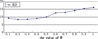
Effect of the value of θ


6.3 Summary
In summary, we draw four conclusions from the experiments as follows.
-
IKD offers scalability and achieves good performance.
-
The run time of both the IKD and the BNL get longer as the radius of query range increases. But IKD performs better than the BNL.
-
The run time of these two algorithms become longer as the number of objects keywords increases.
-
When θ is large, the total run time presents an increasing trend as θ increases. But the total run time will become larger as θ decreases when θ is small.
7 Conclusion
In this paper, we study the skyline problem of fuzzy queries. We only consider the problem of two dimensions, the text relevance dimension and the spatial relevance dimension. We propose two functions to quantify these two kinds of relevance. We also present a new hybrid index structure called Inverted-KD tree and an algorithm based on it to solve the skyline problem. Extensive experimental results show that our algorithm offers scalability and high efficiency.
References
Bao J, Mokbel MF (2013) GeoRank: an efficient location-aware news feed ranking system. In: SIGSPATIA/L GIS 2013. 184–193. ACM, Orlando
Lisi C, Gao C, Xin C (2013) An efficient query indexing mechanism for filtering geo-textual data. In: SIGMOD 2013. 749–760. ACM, NewYork
Long G, Jie S, Htoo Htet A, Kian-Lee T (2015) Efficient continuous top-k spatial keyword queries on road networks. GeoInformatica 19(1):29–60
Huang W, Li G, Tan K-L, Feng J (2012) Efficient safe-region construction for moving top-K spatial keyword queries. In: CIKM 2012. 932–941. ACM, Maui
Chen L, Cong G, Cao X, Tan K-L (2015) Temporal Spatial-Keyword Top-k publish/subscribe. In: ICDE 2015. 255–266. ICDE Press, Seoul
Zheng K, Su H, Zheng B, Shang S, Xu J, Liu J, Zhou X (2015) Interactive Top-k Spatial Keyword queries. In: ICDE 2015. 423–434. ICDE Press, Seoul
Yunjun Gao, Xu Qin, Baihua Zheng, Gang Chen: Efficient Reverse Top-k Boolean Spatial Keyword Queries on Road Networks. IEEE Trans. Knowl. Data Eng. (TKDE) 27(5):1205–1218 (2015)
Zhang D, Chan C-Y, Tan K-L (2014) Processing spatial keyword query as a top-k aggregation query. In: SIGIR 2014. 355–364. ACM, Gold Coast
Chen L, Lin X, Hu H, Jensen CS, Xu J (2015) Answering why-not questions on spatial keyword top-k queries. In: ICDE 2015. 279–290. ICDE Press, Seoul
Tan KL, Eng PK, Ooi BC (2001) Efficient progressive skyline computation. In: VLDB 2001. 301–310. ACM, Roma
Dellis E, Seeger B (2007) Efficient computation of reverse skyline queries. In: VLDB 2007. 291–302. ACM, Vienna
Borzsonyi S, Kossmann D, Stocker K (2001) The skyline operator. In: ICDE 2001. 421–430. ICDE Press, Heidelberg
De Felipe I, Hristidis V, Rishe N (2008) Keyword search on spatial databases. In: ICDE 2008. 656–665. ICDE Press, Washington
Zhang D, Chee YM, Mondal A, Tung AKH, Kitsuregawa M (2009) Keyword search in spatial databases: Towards Searching by Document. In: ICDE 2009. 688–699. ICDE Press, Shanghai
Chen YY, Suel T, Markowetz A (2006) Efficient query processing in geographic web search engines. In: SIGMOD 2006. 277–288. ACM, Chicago
De Felipe I, Hristidis V, Rishe N (2008) Keyword search on spatial databases. In: ICDE 2008. 656–665. ICDE Press, Cancún
Li G, Xu J, Feng J (2012) Keyword-based k-nearest neighbor search in spatial databases. In: CIKM 2012. 2144–2148. ACM, Maui
Xin C, Gao C, Tao G, Jensen CS, Beng Chin O (2015) Efficient processing of spatial group keyword queries. ACM trans. Database Syst (TODS) 40(2):13
Dingming W, Man Lung Y, Jensen CS (2013) Moving spatial keyword queries: Formulation, methods, and analysis. ACM Trans. Database Syst (TODS) 38(1):7
Wang X, Zhang Y, Zhang W, Lin X, Wang W (2015) AP-Tree: Efficiently support continuous spatial-keyword queries over stream. In: ICDE 2015. 1107–1118. ICDE Press, Seoul
Ying L, Jiaheng L, Gao C, Wei W, Cyrus S (2014) Efficient algorithms and cost models for reverse spatial-keyword k-nearest neighbor search. ACM trans. Database Syst (TODS) 39(2):13
Khodaei A, Shahabi C (2012) Chen Li: SKIF-P: a point-based indexing and ranking of web documents for spatial-keyword search. GeoInformatica 16(3):563–596
Jun H, Ju F, Guoliang L, Shanshan C (2012) Top-k Fuzzy Spatial Keyword Search. (in Chinese). Chin J Comput 35(11):2237–2246
Cong G, Jensen CS, Wu D (2009) Efficient Retrieval of the Top-k Most Relevant Spatial Web Objects. In: VLDB 2009. 337–348. ACM, Lyon
Li G, Feng J, Xu J (2012) DESKS: Direction-Aware Spatial Keyword Search. In: ICDE 2012. 474–485. ICDE Press, Washington
Zhang C, Zhang Y, Zhang W, Lin X (2013) Inverted Linear Quadtree: Efficient Top K Spatial Keyword Search. In: ICDE 2013. 901–912. ICDE Press, Brisbane
Yao B, Li F, Hadjieleftheriou M, Hou K (2010) Approximate string search in spatial databases. In: ICDE 2010. 545–556. ICDE Press, Long Beach
Hadjieleftheriou M, Li C (2009) Efficient approximate search on string collections. In: VLDB 2009. 1660–1661. ACM, Lyon
Li C, Lu J, Lu Y (2008) Efficient merging and filtering algorithms for approximate string searches. In: ICDE 2008. 257–266. ICDE Press, Cancún
Xiao C, Wang W, Lin X, Shang H (2009) Top-k set similarity joins. In: ICDE 2009. 916–927. ICDE Press, Shanghai
Kossmann D, Ramsak F, Rost S (2002) Shooting stars in the sky: an online algorithm for skyline queries. In: VLDB 2002. 275–286. ACM, Hong Kong
Papadias D, Fu G, Seeger B, Tao Y (2003) An optimal and progressive algorithm for skyline queries. In: SIGMOD 2003. 467–478. ACM, San Diego
Lee J, Hwang S-W (2014) Toward efficient multidimensional subspace skyline computation. In: VLDB 2014. 129–145. ACM, Hangzhou
Liu B, Chan C-Y (2010) ZINC: Efficient indexing for skyline computation. In: VLDB 2010. 197–207. ACM, Singapore
Acknowledgments
This paper was supported by NGFR 973 grant 2012CB316200, NSFC grant 61472099, 61133002 and National Sci-Tech Support Plan 2015BAH10F01.
Author information
Authors and Affiliations
Corresponding author
Rights and permissions
About this article

Cite this article
Li, J., Wang, H., Li, J. et al. Skyline for geo-textual data. Geoinformatica 20, 453–469 (2016). https://doi.org/10.1007/s10707-015-0243-9
Received:
Revised:
Accepted:
Published:
Issue Date:
DOI: https://doi.org/10.1007/s10707-015-0243-9